Realtime Emotional Reflective User Interface Based on Deep Convolutional Neural Networks and Generative Adversarial Networks

Abstract

It is becoming increasingly apparent that a significant amount of the population suffers from mental health problems, such as stress, depression, and anxiety. These issues are a result of a vast range of factors, such as genetic conditions, social circumstances, and lifestyle influences. A key cause, or contributor, for many people is their work; poor mental state can be exacerbated by jobs and a person’s working environment. Additionally, as the information age continues to burgeon, people are increasingly sedentary in their working lives, spending more of their days seated, and less time moving around. It is a well-known fact that a decrease in physical activity is detrimental to mental well-being. Therefore, the need for innovative research and development to combat negativity early is required. Implementing solutions using Artificial Intelligence has great potential in this field of research. This work proposes a solution to this problem domain, utilising two concepts of Artificial Intelligence, namely, Convolutional Neural Networks and Generative Adversarial Networks. A CNN is trained to accurately predict when an individual is experiencing negative emotions, achieving a top accuracy of 80.38% with a loss of 0.42. A GAN is trained to synthesise images from an input domain that can be attributed to evoking position emotions. A Graphical User Interface is created to display the generated media to users in order to boost mood and reduce feelings of stress. The work demonstrates the capability for using Deep Learning to identify stress and negative mood, and the strategies that can be implemented to reduce them.

1. Introduction

It has been reported by Mind [1] that mental health problems in the UK affect 1 in 4 people, and that 1 in 6 people, in England alone, experience depressive or anxious episodes in any given week. The primary cause of the problem may be singular, but it is often intensified by a multitude of factors. Moreover, a larger percentage of the population occupy office jobs, which are typically very sedentary. It is a well-researched concept that sitting down for longer periods of time and an increase in depressive/anxious mood are correlated. It was found by Kilpatrick et al. [2] that those at work who spent more than six hours a day sitting down experienced elevated rates of depression and anxiety, compared to those who spent less time seated. Although a gradual process, these changes in psychological well-being often become a realisation to people over time. This is where the opportunity for research lies; by monitoring individuals’ emotions on a regular basis in a secondary capacity, i.e., the person can continue with their working activities as normal, stress and negative emotions may be better managed in the short term, leading to reduced long term effects. This work proposes a solution to the identified problem, whereby two concepts of Artificial Intelligence (AI) are combined to, firstly, identify negative emotions, and secondly, to try to reduce their presence. Specifically, a Convolutional Neural Network (CNN) is used to accurately predict when a person is experiencing negative emotions by their facial expressions. Media produced by a Generative Adversarial Network (GAN) is to be shown to the user in an attempt to reduce negative emotions. This paper proposes a novel application for AI and Deep Neural Networks to improve the mental health of system users. The paper explores implementation of a CNN to classify the seven cardinal emotions (Anger, Disgust, Fear, Joy, Neutrality, Sadness, and Surprise) from facial expressions, generation of false images with a GAN, and a Graphical User Interface (GUI) that automatically displays the generated images when a condition is met. Machine and Deep Learning methods are used in conjunction to achieve a classification accuracy of 80.38%, and a varying number of classes for the task are experimented with. The work contributes a novel user interface based on a combination of deep CNN and GAN neural networks that enables real-time reflection of users’ emotional expressions.

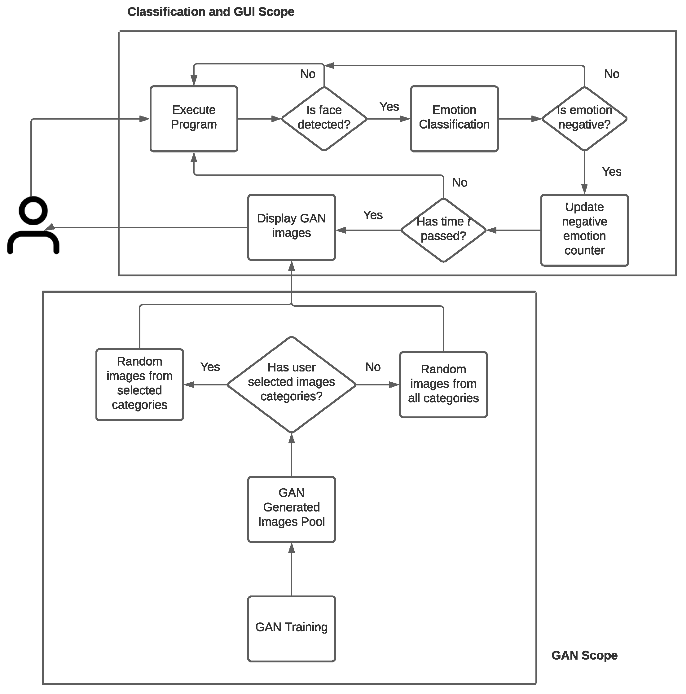
The rest of this paper is organised as follows: Section 2 provides an overview of the available related work, covering facial emotion recognition, Intelligent User Interfaces, Generative Adversarial Networks, and emotion detection in the workplace as an example application. Section 3 explains the system architecture for our proposed solution and how the CNN network interacts with the GAN network. Section 4 discusses the data sets used for this study, Section 5 describes the network architecture of the CNN used, Section 6 explains the training process, Section 7 explains the testing process and results, Section 8 delivers the model optimisation process, Section 9 provides real-time deployment of the model, Section 10 delivers the GAN implementation, Section 11 explains the GUI, the work is discussed in Section 12, and concluded in Section 13 where further work is identified.

2. Related Work

Producing a neural network model capable of accurately classifying emotions from facial expressions is not easily achieved without extensive and representational training data. Images and videos captured for this application area may suffer from poor lighting conditions, varying angles, and proximity to the face; factors such as gender, age, and ethnicity can influence the expression of emotions. Meanwhile, some facial expressions remain subjective, identified differently by separate individuals, and unsuitable to place into a single class. As a result of these issues, numerous methods of data collection and modelling have been implemented by researchers to obtain the best results. Kuo et al. [3] describe the challenges of data collected ‘in-the-wild’, such as lighting conditions and head poses, which can lead to model overfitting. Therefore, to produce a robust deep learning model capable of facial expression recognition, training included the use of various types of data sets. The first, referred to as Set A, were images obtained from laptop webcams capturing three angles. Participants were shown a selection of videos, aimed to produce arousal of the seven common expressions, and afterwards annotated their own images. This is an interesting method as it is likely to be more accurate compared to an observer labelling the displayed emotion. Set B was a collection of images obtained from a Google search of keywords, such as ‘angry/neutral expression’. These were annotated depending on the keyword attached to each image and included a variety of head angles and partial faces. The last set was a grouping of images from movies and television, more complex than set B due to stronger image contrast. This work is illustrative of the different methods that can be used to obtain a wide variety of data.

As Deep Learning (DL) techniques burgeon, the variety of areas in which they can be implemented continues to grow. These advancements are making headway into schools and the workplace to enhance experiences and manage peoples’ well-being. Bobade and Vani [4] present various strategies where Machine Learning (ML) and DL can be used to detect stress levels of people using data obtained from wearable sensing technology. This work used the publicly available data set WESAD (Wearable Stress and Affect Detection) to create deep learning classification models to detect stress. Electrocardiogram (ECG), body temperature, and Blood Volume Pulse (BVP) are some examples of the data in WESAD, and their values fall into one of three classes: amusement, neutral, and stress. A variety of machine learning and deep learning methods, including Random Forest (RF) and Support Vector Machine (SVM), and an Artificial Neural Network (ANN) were compared for performance. It was found that the machine learning methods reached an accuracy of up to 84.32%, comparatively to the ANN, which achieved 95.21%. This work shows the generalisability of trained ML algorithms and DL networks to real world problems, such as detecting the physiological responses to stressful situations. Innovative research combining ML and DL techniques in FER systems have reached high levels of accuracy and generalised well to unseen data.

Ruiz-Gaecia et al. [5] produce a hybrid emotion recognition system for a socially assistive robot that makes use of a Deep CNN (Deep Convolutional Neural Network) and an SVM to achieve an average accuracy score across the 7 cardinal emotions of 96.26%. This specific combination of algorithms achieved the highest score, compared to an average of 95.58% for Gabor filters and SVM; 93.5% for Gabor filters and MLP (Multi-Layer Perceptron); and 91.16% for a combination of CNN and MLP. Achieving accuracy rates north of 90% for facial expression recognition can be considered significant, considering the difficulty of the task. This work shows the advantages in performance where a combination of techniques is used. A further useful application of such techniques is the monitoring of driver concentration levels in vehicles.

Natio et al. [6] aimed to identify when a driver was drowsy from their facial expressions using recordings obtained from a 3D camera. Participants used a driving simulator for five hours each whilst in a dark room, during which they were wearing an Electroencephalograph (EEG) to measure frequency of brain wave activity. This was performed to categorise two states: drowsy, and awake. The 3D camera captured 78 points on participants’ faces at 30 Frames Per Second (FPS), and these were used to visually support the labelling of each state from data captured by the EEG. Using K-Nearest Neighbour (KNN) algorithm, the work achieved 94.4% accuracy. This work is demonstrative of the supporting evidence facial expressions can provide when using other types of data to train machine learning models.

Goodfellow et al. [7] proposed a zero-sum game concept in order to sufficiently train generator algorithms to reproduce similar data to an existing training set. The framework was coined as a Generative Adversarial Network (GAN), and it works in the described way. A Generator model takes a fixed-length random vector, which is taken from a Gaussian distribution, as input and produces a sample within this domain. A normal classification model, known as the Discriminator, classifies each image as fake or real (0 or 1), and its weights are updated during training to improve its classification performance. The Generator is updated depending on how well its generated samples have fooled the Discriminator; when the Discriminator successfully classifies the generated samples, the Generator is penalised with large parameter updates.

The current SOTA GAN architecture performance can be attributed to the work by Karras et al. [8]. The research implements improvements to address some issues identified with images produced by StyleGAN. For example, smudge-like areas could be seen on all generated images above 64x64 resolution; the authors attribute this to the use of Adaptive Instance Normalisation (AdaIN), where mean and variance values of each feature map are normalised, causing a destruction of data. To combat such issues, the work re-engineered generator normalisation with regularisation, and progressive growing. The work achieved SOTA performance, such as an FID score of 2.32 on the LSUN Car data set (Yu et al. [9]).

Johnston et al. [10] identified the standardised process for the creation of IUIs as an under-researched area. The work aims to improve user experience universally through provision of a framework for the development of IUIs. Specifically, it looks to combine the dynamic, adaptive, and intelligent components of intelligent interface development. Dynamic elements are responsible for providing basic user experience, and are referred to as being understanding of the user, along with the device and environment. Secondly, adaptive elements allow for recognition of the user’s activity pipeline, and cover usability and accessibility aimed at enhancing user experience. Machine Learning algorithms are implemented to develop intelligent components of IUIs; they are used to interact specifically with the user’s interests, preferences and ease their workload. Intelligent components have an understanding of the user’s end goal whilst using an application. The work argues that introducing a standardised framework to this field would inevitably improve the journey through an application, thus reducing cognitive load for users. The authors also discuss methods of testing when systems are built using a standardised framework, such as gaze and eye tracking with sensor technology, and electroencephalography to analyse brain activity. This work also identifies that using ML to assist the adaptability of user interfaces is a limited area of research.

Liu et al. [11] developed an Adaptive User Interface (AUI) that is based on Episode Identification and Association (EIA). This concept refers to the interface recognition of a user’s actions prior to them being carried out. This is achieved through trace and analysis of action sequences created by the system observing interaction between user and application. Episodes are derived from sets of actions to create classes, such as typing, menu selection, pressing of buttons. This allows for recognition in user behaviour patterns, meaning that the system is able to provide assistance preemptively. To test their proposed work, the study developed an AUI using applied EIA under an existing, sophisticated application, Microsoft Word. The interface provides assistance in two forms: firstly, it boasts a phrase association, where words inputted by the user are treated as parts of an episode, storing up to five words. This enables word and phrase suggestion to the user. Secondly, it offers assistance to help with paragraph construction by identifying commonly used configurations, such as changing the font size, or changing text to bold. The system was tested by nontechnical university staff and students, and the research recorded acceptance rates by user for phrase association at 75%, and format automation at 86%. Feedback was gathered through completion of a questionnaire for participants to rate their experience with the system; on a scale of 1 (very poor) and 7 (very good), the phrase association was rated at 5.78, and for format automation, 5.69, for quality measure. The study also concluded that usage of the system increased individuals’ productivity, for a test and control group comparatively.

Stumpt et al. [12] conducted a study that analysed the effect that real-time user feedback via keyboard input had on training of a Neural Network, particularly in cases where training data is limited. Forty-three English-speaking University students who were proficient in using email were to classify 1151 emails into appropriate folders given their content. The purpose of the work was to investigate the concept of Programming by Demonstration, whereby the end-user of a system is able to teach a machine patterns of behaviour through demonstration. The work developed an email application that is demonstrative of how interaction between ML and end users can improve predictions; the classifier ‘explains’ its reasoning for outputting a prediction, alongside providing ways that the user can give feedback. It makes use of a ‘feedback panel’, where users can update the words found in emails they want the classifier to consider as keywords, remove words from the keyword watch-list, and attach a weighted value to each word using a slider function. The authors liken this approach to User Co-training, seen in semi-supervised learning, where two classifiers use different features of the same data to classify samples. Labelled data is used at first for training, then they are tested on unseen data. The samples classified with the highest confidence are appropriately labelled and appended to the training set for further training. In this study, the user acts as a classifier which is responsible for labelling data for the alternate classifier, the Naive Bayes algorithm. The work concluded that providing the user with feedback from the classifier is beneficial to them, and providing the classifier with rich user feedback aids to improve accuracy considerably.

Research into the emotional well-being of employees in the workplace remains a well-populated field of research. Technology and AI can play significant parts in the capture and analysis of real-time data to better understand the working environment. Chandraprabha et al. [13] proposed RtEED (Real time-Employee Emotion Detection system), which uses ML to detect real-time emotions, and a messaging system to make employees aware of their overall emotional well-being during the working day. Data was captured through employee webcams and the CNN was engineered to classify six emotions, namely happiness, sadness, surprise, fear, disgust, and anger. The work also developed a GUI to display information to the end user. For example, members of staff can navigate the interface and view the consolidated percentage of emotions expressed by a specific employee.

Yan et al. [14] carried out research into Mental Illness among employees in health care settings, and developed a solution to aid self-assessment of mental status, and encourage early detection of work-related stress and mental illness. In their research, 352 medical staff completed psychological assessments, such as the Emotional Labour and Mental Health questionnaire. This was designed to assess employees in two major areas: firstly, their ability to deal with any external changes at work, and secondly, their internal resilience and endurance to hardship at work. When an employee scores a high probability in the various categories of questions, a classifier outputs 1 of 4 classes, and is then prompted to see a specialist for help if classification is of a certain class.

Walambe et al. [15] discuss that mental health and well-being remains a neglected part of peoples’ lives, even though the impact can be so significant. Although it is crucial, identifying stress levels and pinpointing the trends is challenging, and often relies on many factors. Therefore, a better solution is needed; however, the work explains that solutions implementing Machine and Deep Learning for this task are very few. The research proposes a multi-modal AI framework to monitor behaviour and stress levels at work. This is achieved through the concatenation of various data collected by sensors, such as facial expressions, pose and posture, heart rate, and interaction with computers. Capturing and analysing such data enabled the detection of stress and behavioural patterns of employees. The work achieves 96.67% test accuracy in classification.

3. System Architecture

The objectives of the work will be achieved through the implementation of various concepts. Firstly, a CNN will be trained on a vast database of images to detect the differences between facial features for various emotions. The network will be optimised using several strategies, and a wide range of implementation experimented with to achieve the best possible results. The optimised model, reaching the best performance metrics, and its’ weights, will be saved and deployed to capture and classify facial expressions via live webcam. A timer will start when a face is detected in the camera frame, and if specified emotions are detected by the classifier, after a time threshold, a Graphical User Interface (GUI) will be shown to the user. This will enable browsing of images intended to improve mood. The images are false data, generated prior to this by a GAN. The system architecture is illustrated in Figure 1. The work experiments with three different Models, whereby the number of classes is altered for each.

4. Data

The data set of images used in CNN development is a combination of several, existing data sets. They are all representational of the seven cardinal emotions: Anger, Disgust, Fear, Joy, Neutrality, Sadness and Surprise. This approach was taken due to the need for large quantities of data to train CNNs effectively to increase their generalisability to unseen data. This specific task remains well studied in the Deep Learning (DL) field; Hu et al. [16] studied the effects of using smaller data sets to train models and were able to conclude that significantly high accuracy rates are consistent when training models with as few as 10,000 images. Although this is a relatively small number to use for training, there are few existing data sets of this size consisting of images where: facial occlusion is minimal; ethnicities of people are varied; and faces are centralised in images. For this reason, a data set was created to minimise these disadvantages. The total number of images in our final data set is 40,972. The following describes each data set used.

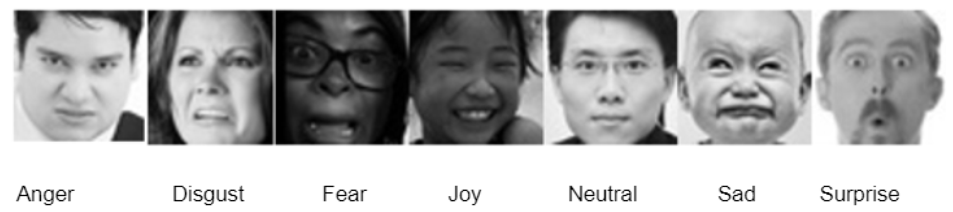
FER-2013 or Facial Emotion Recognition-2013 is the largest contributor for our data set (Kaggle [17]), comprising 25,702 sample images for training, and 6726 for testing. The faces are reasonably well centred in the images, occupying a similar amount of space in each. This data set can be described as well representational of facial expressions in-the-wild. In comparison to others, Minaee et al. [18] advocates that it contains the most variation, with features such as partial faces, images of low contrast, people wearing hats or glasses, and facial occlusion where the hand of the person is also shown. It is inclusive of infants, children, and adults; males and females; and includes a variety of ethnicities. See Figure 2 for examples.

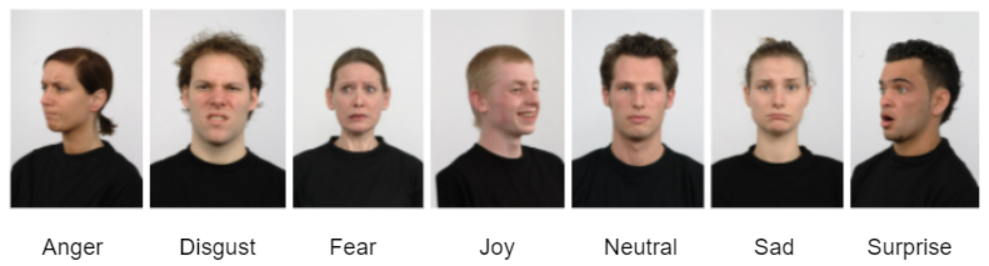
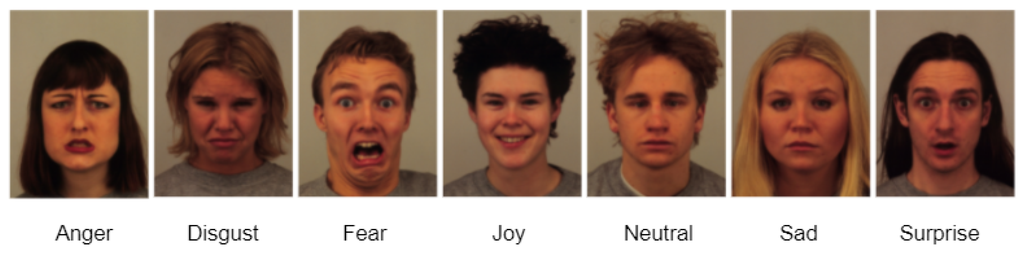
The Radboud Faces Database (Langner et al. [19]) contributes a total of 4403 images. This database comprises 67 actors, including males and females, adults and children, Caucasian and Moroccan-Dutch ethnicities, displaying a total of eight emotions: Anger, Disgust, Fear, Joy, Neutral, Sadness, Surprise, and Contempt. All images are sized at 681x1024 and are in colour. The images used from this source are not inclusive of the Contempt class and show three different camera angles only: head facing the camera, head angled roughly 45 degrees to the left, head angled roughly 45 degrees to the right. See Figure 3 for examples.

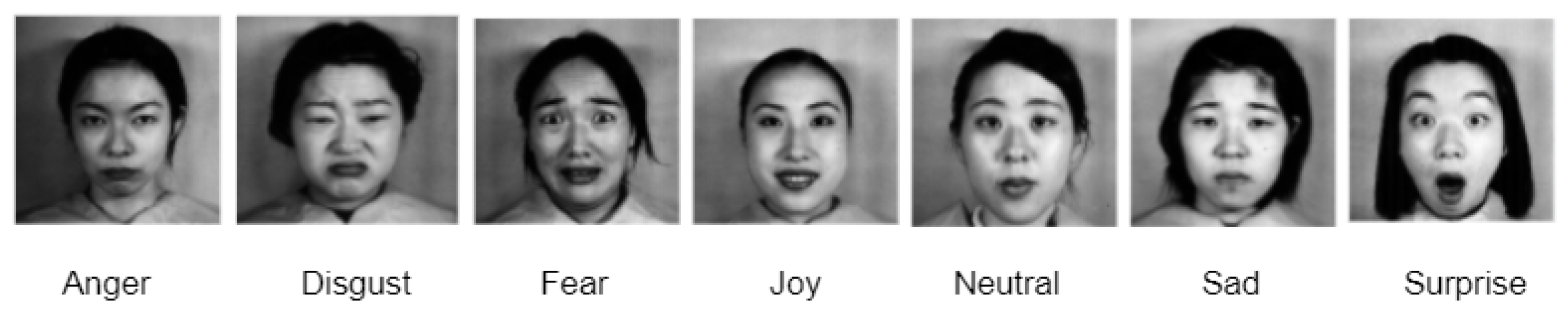
The next data set used was the Japanese Female Facial Expression (JAFFE) Database (Lyons et al. [20]). A total of 213 images of 10 female actors are included. The images are in greyscale, of size 256 × 256, and some offer better lighting than others. For example, some images include a shadow over the actors’ face, compared to others where the entire face is brighter, thus facial features such as eyes and mouth are clearer. See Figure 4 for examples.

The Karolinska Directed Emotional Faces (KDEF) data set (Lundqvist et al. [21]) contains seven emotions expressed by 70 individuals, each expression captured at five separate angles. However, for this study, this data set has contributed three of those five angles which are most suited to the task. All images from this data set are sized at 562 × 762 and are in colour. The unused images from the database consisted of the faces turned completely to the right or left, which are not suitable for the task. See Figure 5 for examples.

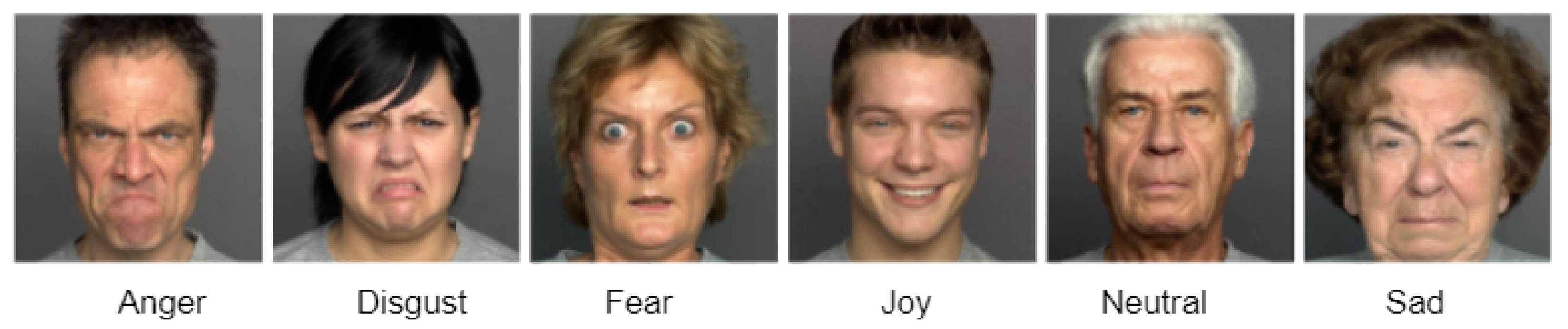
FACES database (Ebner et al. [22]) consists of naturalistic emotions, expressed by six individuals in the publicly available version, totalling 72 images, sized 200 × 200 × 3. This data set contains only six emotions: Anger, Disgust, Fear, Joy, Neutrality, and Sadness. These images were included in the work due to their strong similarity to other, larger data sets used, such as KDEF. See Figure 6 for examples.

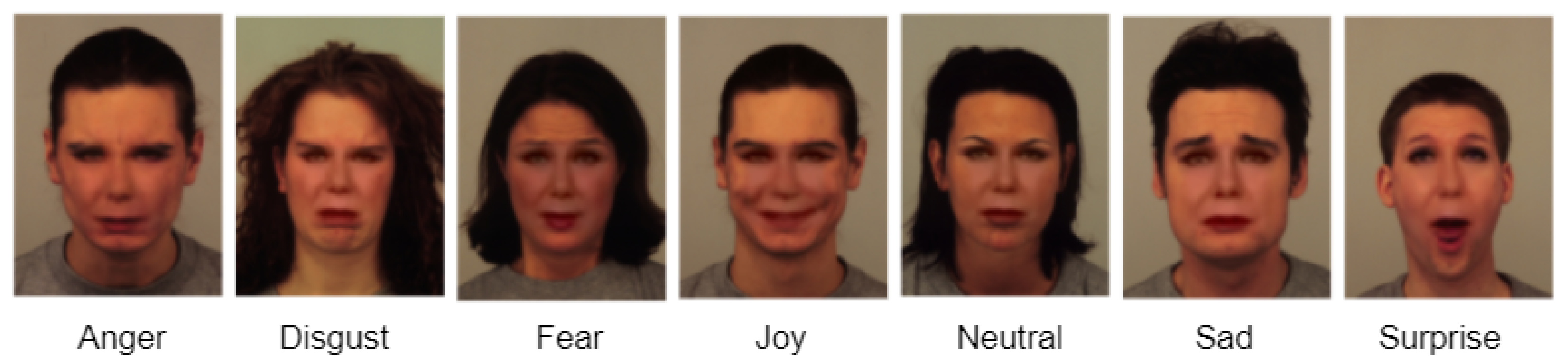
GAN Generated KDEF is another contributor data set (Porcu et al. [23]) containing similar images to the KDEF data set created using a Generative Adversarial Network (GAN). This technique enabled the training data to expand in size, thus improving performance. The generated images are a considerable size at 562 × 762 × 3. Using these false images increased the size of the overall data set by 980. Although the images are not visually perfect, it is understandable which emotion is being expressed. See Figure 7 for examples.

We created a data set for this work using images extracted and integrated from six existing data sets.

Table 1. Breakdown of data for the created dataset.

Dataset	Number of Training Images	Number of Testing Images
FER-2013	25,702	6726
JAFFE	168	45
FACES	48	24
KDEF	2810	66
RADBOUD	4201	202
KDEF GAN Generated	779	201
Total	33,708	7264

shows the contribution from each original data set, divided between test and training.

Upon inspection, a significant imbalance in the number of data samples between classes was identified. A consistent pattern emerged, where classes such as Neutral and Joy were overpopulated, and Disgust showed the fewest samples by almost 5 times. Data sets displaying a large imbalance between classes will likely cause issues for the classifier during training, thus affecting its generalisability; Johnson and Khoshgoftaar [24] explain that when an imbalance exists, Deep Learning models tend to over-classify samples into the majority class. This results in samples of the minority class being classified incorrectly at a high frequency, compared to the class with the greatest number of samples. This will inevitably create a network with poor testing performance. Data Augmentation is a method that can be applied to images in specific classes to increase the size of training samples. Applying multiple geometric transformations to existing images improves not only the quantity of images, but also the variety. For example, taking an original image and introducing Gaussian noise, or rotating it 45 degrees, provides the network with a variation in similar features to learn. 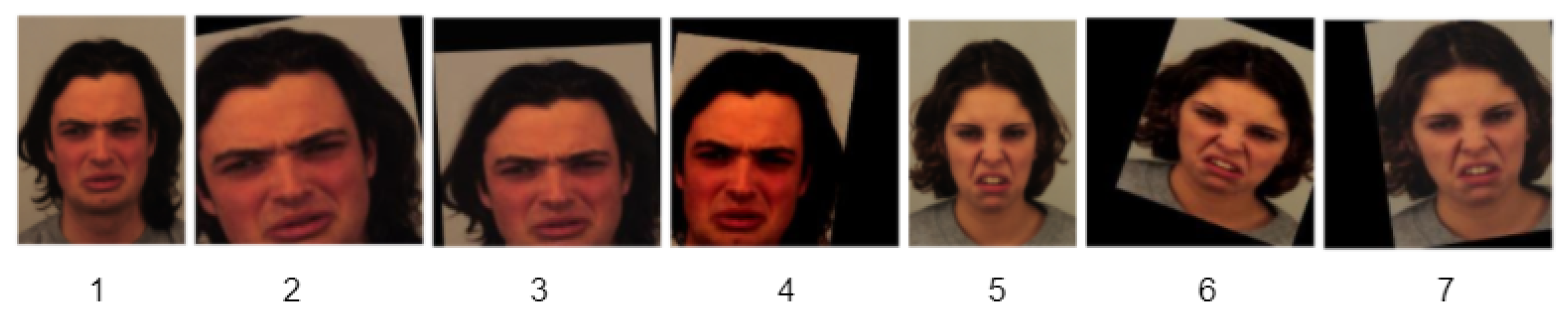Although a traditional approach, artificial inflation of the training data using these techniques remains a reliable way to improve accuracy of classification; Taylor and Nitschke [25] evaluated their results using 4-fold cross-validation and concluded that applying cropping to training data reliably and significant improves performance of CNNs. Data Augmentation was applied to the Disgust class to increase its’ count towards a number closer to the mean, 4815. Transformations were implemented in a random order and included cropping, Gaussian blur, linear contrast, rotation, translation, and scaling. The number of augmentations applied was three; for each original image used, three new samples were created. Examples are shown in Figure 8.

The first three augmented examples show that the images have been cropped; the first and second augmented images show Gaussian noise, where the face appears somewhat stretched horizontally; the contrast has been altered for the last image, where the skin tone appears different; the images also show a varying amount of rotation. Augmentation of the original Disgust class images increased sample size by 3252 images, totalling 4757. A significant class imbalance also appears in the data used for Models B and C. To target this issue and reduce the problems it might cause, the same augmentation methods were applied to the Neutral and Positive classes, specifying two augmentations per image used in the process.

5. CNN Models

The network architecture comprises five convolutional layers, using 16, 32, 64, 128, and 128 filters as the network depth increases by each layer. The filters are all sized at 3 × 3. Each convolutional layer makes use of Rectified Linear Unit (ReLU) as its’ activation function and uses ‘same’ padding, to ensure the shape of the input and output data are the same. Each convolutional layer is followed by a layer implementing Batch Normalisation. Then, Max Pooling is applied, using a pool size of 2 × 2. After these 5 blocks, the inputs are flattened so are fed into the subsequent parts of the architecture one by one. The last block of the network makes use of three Dense layers, with 256, 128, and 64 neurons, each followed by a Batch Normalisation layer. This section of architecture also has two Dropout layers, using values of 0.8 and 0.4. The classification layer makes use of 7 neurons, one for each of the potential output classes and uses softmax activation function to output a probability distribution for all classes for each given sample.

Optimisation algorithms are used to enhance the performance of networks during training and increase the rate at which they reach convergence. Adam optimiser, introduced by Kingma and Ba [26], is an optimisation method for stochastic objective functions that offers computationally efficient benefits. Tato and Nkambou [27] explain that it works by scaling the Learning Rate (LR) for all parameters using the exponential moving average of gradients. The hyperparameters used in Adam for the network were initialised as follows:

Learning Rate = 0.001, Beta 1 = 0.9, Beta 2 = 0.999, Epsilon = 1 $\times {10}^{-8}$

The length of time required to train networks to a good standard is often very long. This is exacerbated by a multitude of factors, such as the amount of training data; the size and colour dimensionality of images; depth of the network; batch size; hardware capabilities; and power supply. The number of iterations through the data set is what ultimately determines the training time, known as epochs. Whilst a large number of epochs is required to sufficiently train, instances may occur where global minima has been reached many epochs before the total number set is reached. This can cause engineers to lose time, efforts, and resources, whilst potentially resulting in an overfitting model. Therefore, the method of Early Stopping has been implemented to avoid such occurrences. With Early Stopping, an arbitrary number of epochs is set, the patience value, which halts training early if a condition has been met. This method monitors the specified metric (accuracy or loss) and will stop training if the metric has not improved once the patience value has been reached. For example, a network that outputs 5 epochs during training which all display a consistent increase in validation loss will stop training early, providing that the patience value is 5 and the monitored metric is validation loss. The implementation of Early Stopping in this work monitored validation loss, with a patience value of 15.

It is necessary to validate the performance of a neural network as it trains; Shah [28] explains that this provides an evaluation of how the network is fitting to the training data at that current time of training which is unbiased. The performance metrics scored on the validation set are more reliable in relation to how the model might perform on unseen data. We use 5-Fold cross-validation during the training process to thoroughly evaluate the performance of the model. This is where the data set is separated into five separate folds, and as each fold is iterated in training, a different fold is used to validate the model performance in terms of accuracy and loss, and the remaining folds used for training. Each fold will contribute to training, as well as acting as the test set once. K-Fold validation ensures all available data for training is utilised, and a less biased validation performance is yielded. It is also important to ensure the shuffle parameter for this method is set to True. This ensures that the entire training data set is shuffled prior to any division. If this parameter is not specified and shuffling does not occur, it can result in bias towards one class, which will cause unreliable model performance.

6. Training

The paper experimented with three Models in relation to CNN training, which involved using the same data, but dividing it into a different number of classes for each. This was completed to maximise experimentation and investigate the best method to apply to the task. Additionally, this field of research is typically dominated by classifying expressions into seven classes. This is necessary when all classes are relevant to the application, however, the objectives of this research enable flexibility in this approach.

Model A experimented with multi-class classification, where all seven classes for determining emotion were used. The total number of training images for this Model is 36,960. Details of the experiments carried out for this Model can be found in

Table 2. Model A training and validation results.

	Img Size	Batch Size	# Parameters	Train Acc (~)	Train Loss (~)	Val Acc	Val Loss
1	200 × 200 × 3	32	1,469,799	79%	0.52	67.82%	0.89
2	300 × 300 × 1	32	2,944,071	78%	0.73	66.95%	0.91
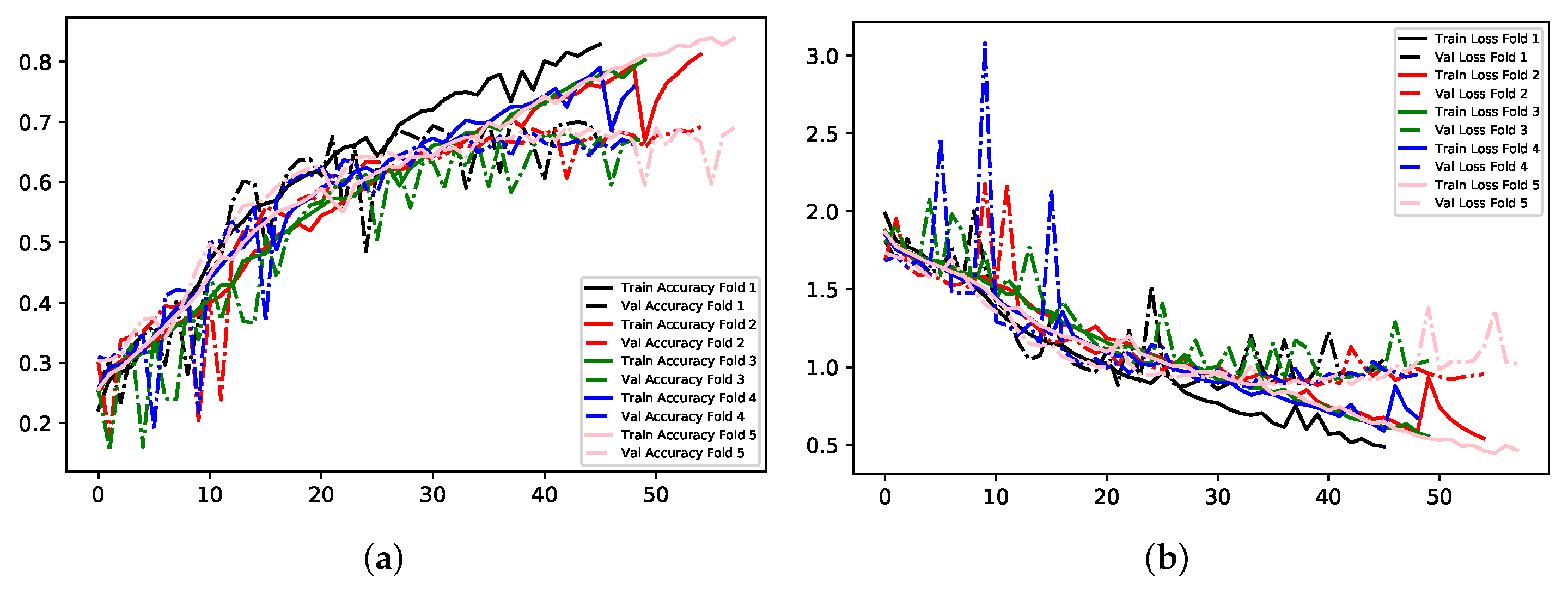
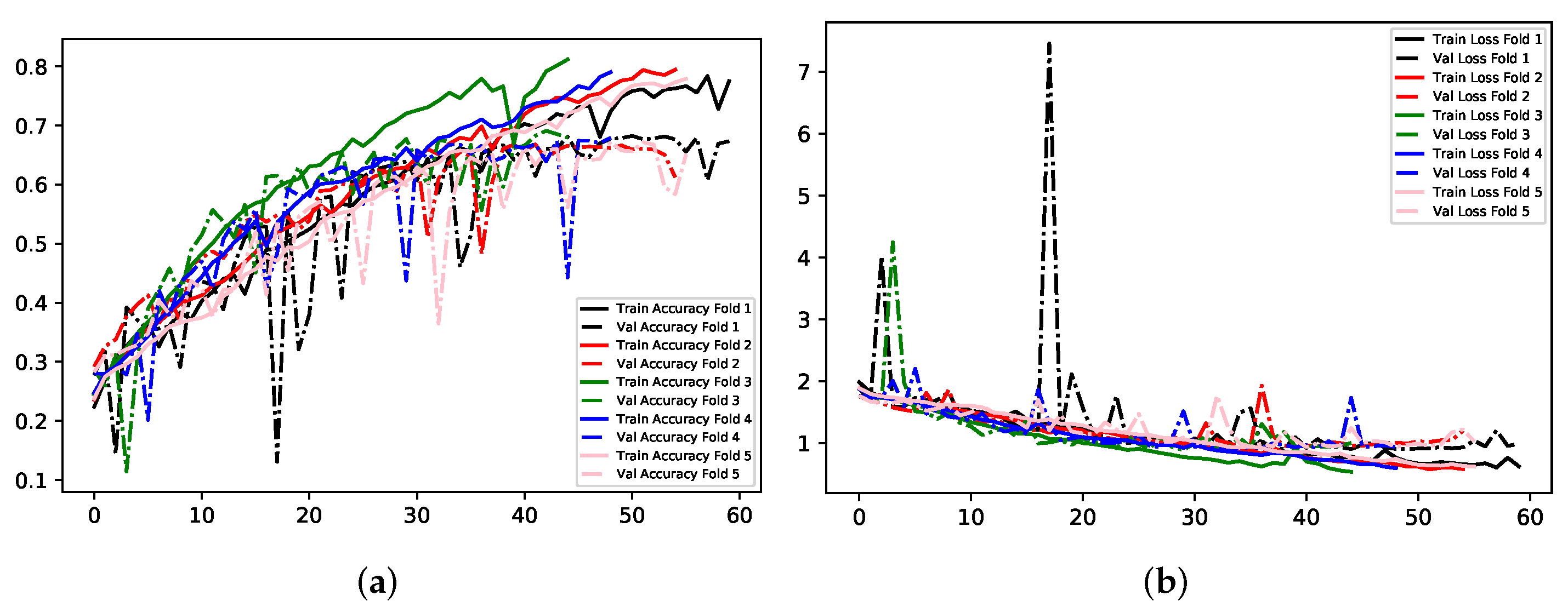
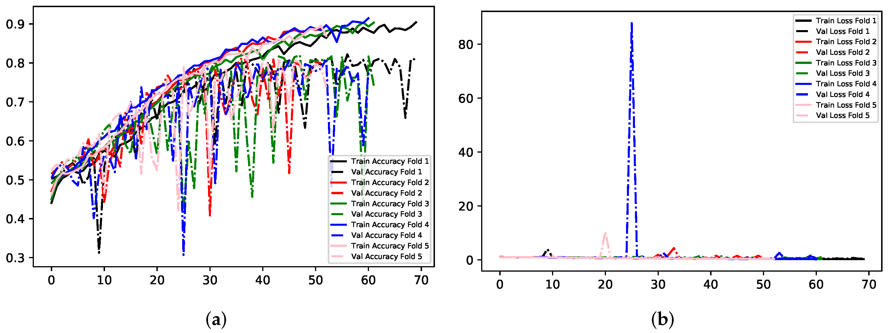
3	224 × 224 × 3	32	3,236,039	50%	1.31	47.89%	1.36

. The batch size configured for these experiments was set to 32, alongside a total of 70 epochs. As aforementioned, Early Stopping was used with a patience value of 15 to prevent wasting time with ineffective training, and to avoid an overfitting network. Firstly, images sized at 200 × 200 and in RGB were used for training the CNN. The results show an overfitting model regarding accuracy scores, with a training accuracy and loss of approximately 79% and 0.52 respectively. This is compared to a validation accuracy of 67.82% and validation loss of 0.89. The second experiment passed the images into the neural network in greyscale, and with a larger size than the previous, at 300 × 300. The batch size and total number of epochs remained the same as 32 and 70 respectively. This model also shows an amount of overfitting: in training it achieved 78% accuracy, compared to validation accuracy of 66.95%. Training loss was 0.73, compared to validation loss of 0.91. This model has a worse performance across the board than the previous.

Finally, Transfer Learning was implemented using MobileNet. Transfer Learning is the concept of efficiently completing a new task by transferring the abilities, knowledge, and skills of a related task. For example, image classification requires networks to be able to detect edges in the input data; although the classes are specific to the task, the process of identifying the key characteristics may be transferrable to tasks in different domains. Additionally, Weiss et al. [29] offer that using models that have been trained on a large amount of data, inclusive of a variety of classes, reduces the need for collecting new data for every task, as this is very time and resource expensive. Proposed by Howard et al. [30], MobileNet was chosen to experiment with due to its small comparative size at 4,253,864 parameters. Arguably, larger networks boasting more parameters would have likely outperformed MobileNet for this task. However, making use of a smaller network allows for a reduction in required computation and resources. Various factors influenced this decision; given that the images as input are medium in size; there are a considerable number to feed through the network; and the research is somewhat constrained by hardware capabilities. 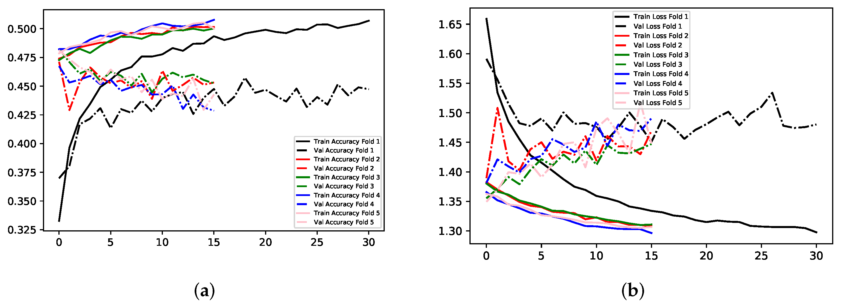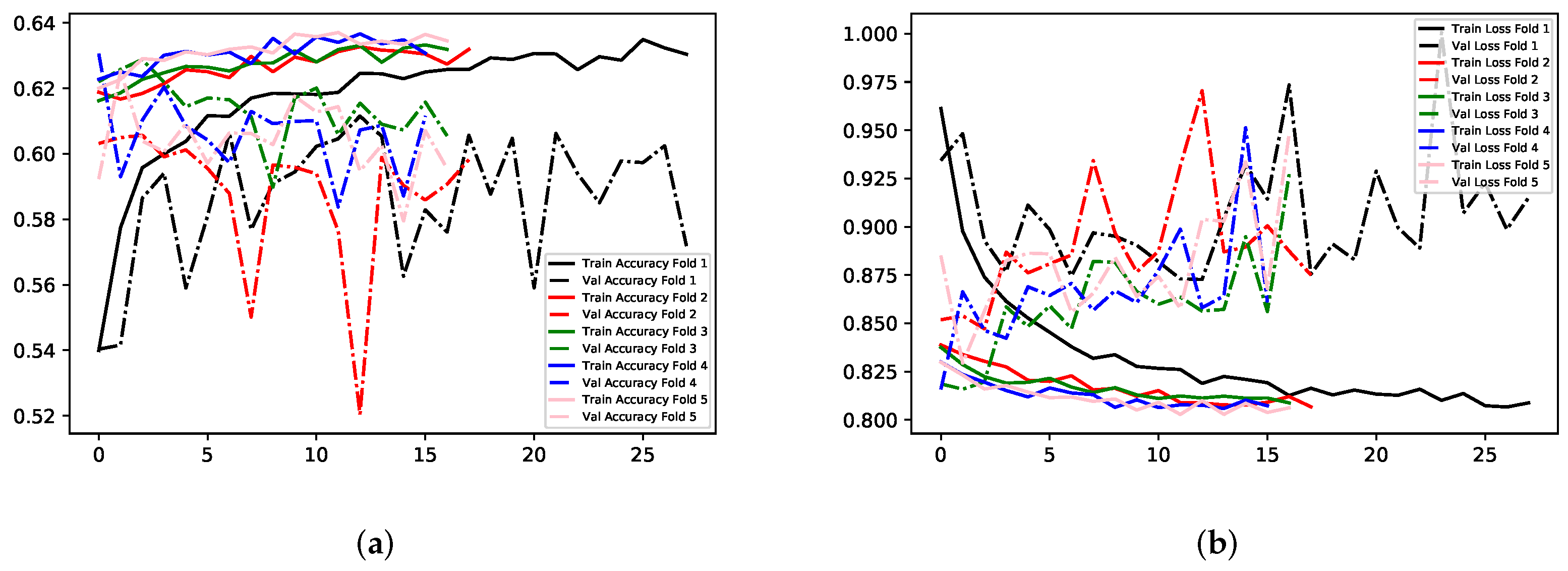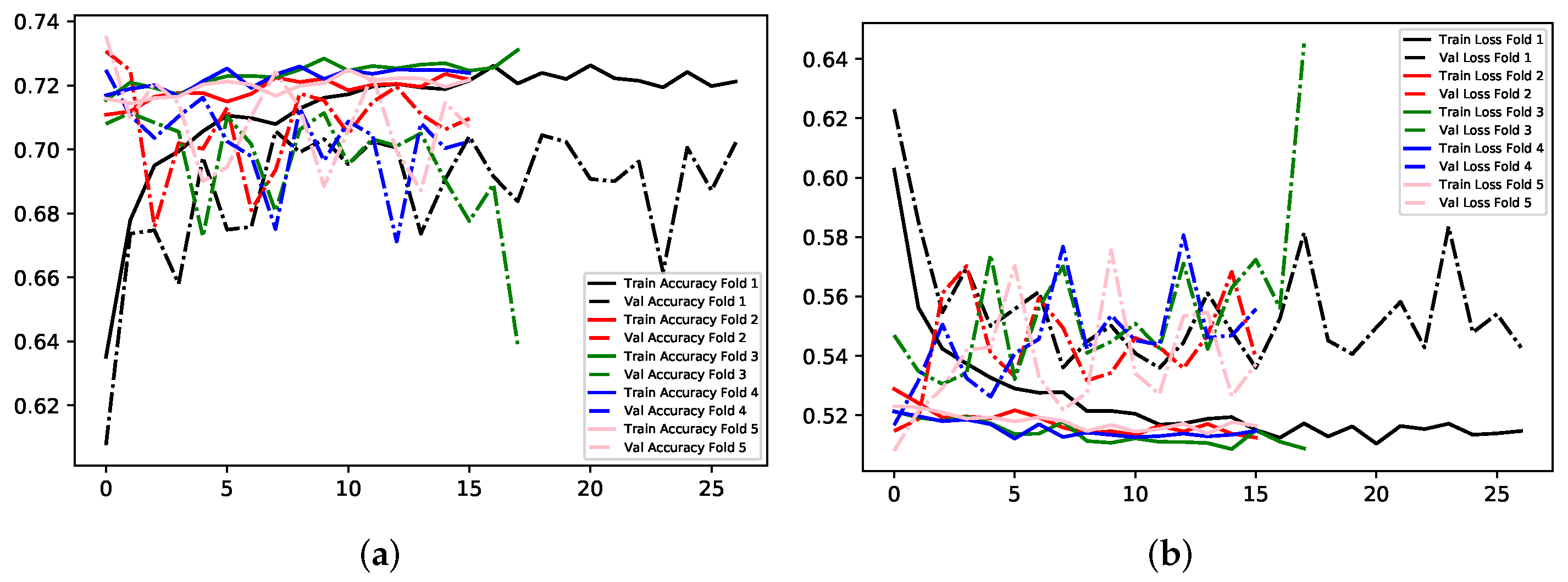It is shown in Table 2 that using MobileNet for Transfer Learning yielded the most modest performance. Images were sized at 224 × 224 × 3, and the batch sized remained at 32. Although the poorest performer, this method showed the least amount of overfitting, with small differences in accuracy and loss for training and validation. Experiment 1 yielded the best results for this Model.

Figure 9, Figure 10 and Figure 11 illustrate the comparisons between accuracy and loss for training and validation for the three experiments. Experiments 1 and 2 show a general trend throughout training and validation, with several occurrences of anomalies. Experiment 3 demonstrates instability in each validation fold until training ceases.

Model B involved the use of three classes: Negative, Neutral, Positive. This used the same image data as the previous, with only the exclusion of the Surprise class. This class was negated from the data set for Models B and C, due to its’ ambiguity. Surprise can have negative or positive connotations, and is usually dependent upon the expressing individual, as well as any observers. Therefore, it was unsuitable to include. This method of classification was derived from the theory that this application domain may not require seven classes for the desired outcome of the research. To improve mood whilst working, it may only be necessary to differentiate between negative, positive, and neutral expressions. Thus, it may be more efficient to concatenate negative emotions, Anger, Disgust, Fear, and Sadness, into one large class, whilst the remaining two classes represent positive emotions, and neutral expressions. Details showing the number of images for the Negative class, and the type of negative emotion, are shown in

Table 3. Training data for negative class (Model B).

	FER-2013	JAFFE	FACES	KDEF	RADBOUD	KDEF GAN Generated	Total
Anger	3241	23	9	397	758	106	4534
Disgust	398	23	9	390	575	111	1506
Fear	3515	28	8	404	574	106	4635
Sadness	4408	25	9	407	573	111	5533
Negative	11,562	99	35	1598	2480	434	16,208

. Refer to

Table 4. Training data for positive and neutral classes (Model B).

	FER-2013	JAFFE	FACES	KDEF	RADBOUD	KDEF GAN Generated	Total
Neutral	4474	22	6	1498	1673	1213	8886
Joy/Positive	6688	22	7	1139	1305	849	10,010
Total	11,162	44	13	2637	2978	2062	18,896

for details of Neutral and Positive classes. The total number of training images is 35,104.

The same experimental methods were used to train the network for this Model. Refer to

Table 5. Model B training and validation results.

	Image Size	Batch Size	# Parameters	Train Acc (~)	Train Loss (~)	Val Acc	Val Loss
1	200 × 200 × 3	32	1,469,539	90%	0.25	81.86%	0.44
2	300 × 300 × 1	32	2,946,811	89%	0.16	81.18%	0.47
3	224 × 224 × 3	32	3,228,864	63%	0.81	61.72%	0.83

for all training and validation results.

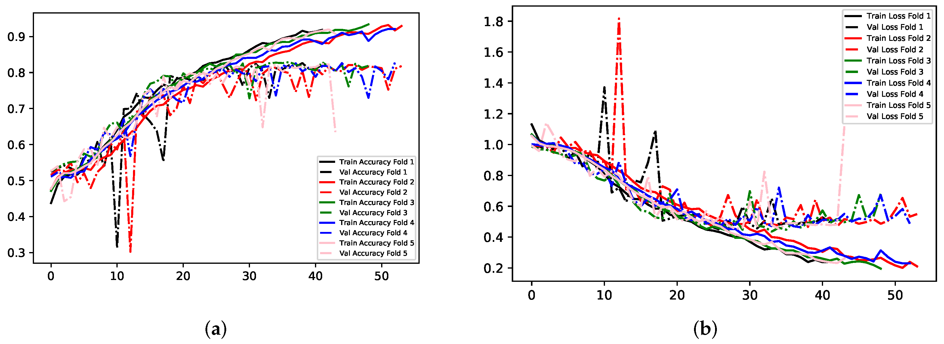
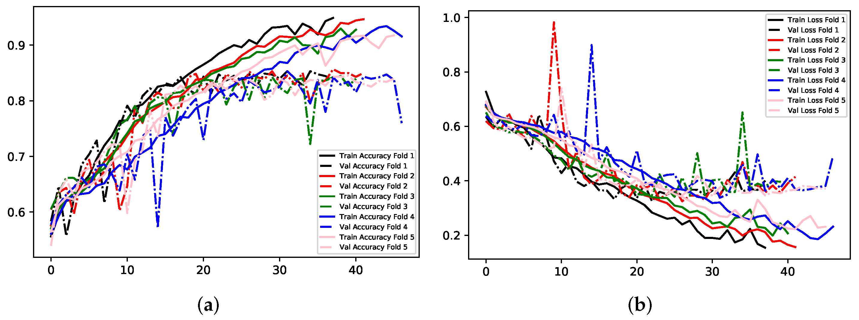
The training behaviour in experiment 1 showed similarities to the same experiment in the previous in that it overfits to the training data considerably. However, altering the number of classes for the problem has shown a dramatic increase in validation accuracy in comparison to experiments with Model A; concatenating negative emotions into one class enabled 81.86% and 0.44 validation accuracy and loss respectively for experiment 1. Using images sized at 300 × 300 × 1 with data divided into three classes yielded 89% and 81.18% accuracy for training and validation respectively. Transfer Learning with MobileNet, again, showed the least amount of overfitting across experiments for this Model; just 1.28% separates the accuracy scores for training and validation, and 0.02 for the two loss values. Experiment 1 yielded the best results. See Figure 12, Figure 13 and Figure 14.

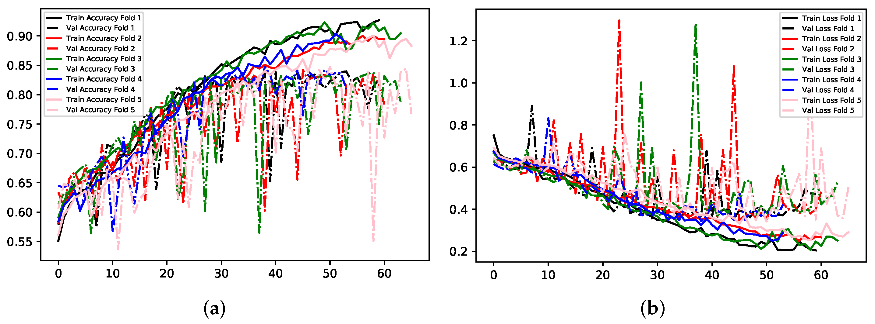
Model C uses binary classification, where images fit into one of two classes, Negative and Positive. This implementation used exactly the data of that in Model B. Therefore, the only difference is that images belonging to Neutral before, are now grouped with Positive. This method of classification derives from the possibility that Neutral as a standalone class may not be required for the application. It can be argued that for most of the time, people have a neutral expression when using computers, which somewhat negates the requirement to identify it. This was handled by grouping it into the Positive class. All experimental techniques implemented so far vastly improved with this Model. Images sized at 200 × 200 × 3 were able to yield the highest accuracy with a low loss value on the validation set, 84.85% and 0.33 respectively, although this experiment demonstrates an amount of overfitting. Secondly, images sized 300 × 300 × 1 achieved a similar, but not quite as good, performance as the previous, with validation accuracy and loss at 83.74% and 0.35 respectively. These results also indicate an amount of overfitting. Images were sized 224 × 224 × 3 for TL with MobileNet, resulting in similar metrics; MobileNet is the underachiever for all Models, with a validation accuracy and loss of 72.11% and 0.51 respectively. Experiment 1 yielded the best results for this Model. All results can be found in

Table 6. Model C training and validation results.

	Image Size	Batch Size	# Parameters	Train Acc (~)	Train Loss (~)	Val Acc	Val Loss
1	200 × 200 × 3	32	1,469,474	91%	0.22	84.85%	0.33
2	300 × 300 × 1	32	2,943,746	90%	0.23	83.74%	0.35
3	224 × 224 × 3	32	3,228,864	72%	0.53	72.11%	0.51

, with visual representation provided in Figure 15, Figure 16 and Figure 17.

7. Testing

Model A, Seven Classes: The testing data set for the first Model tells a similar story to the training data; FER-2013 is the largest contributor; Joy class dominates with a total of 1817 images; and Disgust class has the fewest, at 180. The mean number of images per class is 1038, where the Fear class sample count is closest to this distribution, whereas Disgust and Surprise deviate in large and medium quantities respectively. The total number of testing images for this model is 7264, refer to

Table 7. Testing Data (Model A).

	Anger	Disgust	Fear	Joy	Neutral	Sadness	Surprise	Total
FER-2013	847	107	979	1732	1137	1121	803	6726
JAFFE	7	6	4	9	8	6	5	45
FACES	3	3	4	5	6	3	0	24
KDEF	10	8	8	10	11	10	9	66
RADBOUD	30	27	28	34	25	30	28	202
KDEF GAN Generated	34	29	34	27	23	29	25	201
Total	931	180	1057	1817	1210	1199	870	7264

for the breakdown.

Model B, Three Classes: As with the training data for this Model, the emotion labels with negative connotations, were concatenated to form the Negative class. This partition is dominated by images expressing Sadness and has the fewest samples expressing Disgust. The Surprise class has been negated for testing of Models B and C.

Table 8. Testing Data for Negative Class (Model B).

	FER-2013	JAFFE	FACES	KDEF	RADBOUD	KDEF GAN Generated	Total
Anger	847	7	3	10	30	34	931
Disgust	107	6	3	8	27	29	180
Fear	979	4	4	8	28	34	1057
Sadness	1121	6	3	10	30	29	1199
Negative	3054	23	13	36	115	126	3367

displays details for Negative class, refer to

Table 9. Testing Data for Positive and Neutral Classes (Model B).

	FER-2013	JAFFE	FACES	KDEF	RADBOUD	KDEF GAN Generated	Total
Neutral	1137	8	6	11	25	23	1210
Joy/Positive	1732	9	5	10	34	27	1818
Total	2869	17	11	21	59	50	3028

for details of Neutral and Positive classes. The total number of testing images is 6395.

Model C, Binary Classification: The data set used to test the models for the binary classification Model mirrors that used to test Model B. Therefore, details found in Table 8 represent the Negative class for testing binary classification method. Refer to Table 9 for the breakdown of the Positive class for testing, simply concatenate neutral and joy to form the Positive class. The total number of testing images is 6395.

Table 10. Testing Accuracy and Loss Values (All Models).

	Experiment	Test Accuracy (%)	Test Loss
(A) 7 Classes	1:RGB	59.09	1.13
	2:GREY	58.71	1.15
	3:TL	39.88	1.58
(B) 3 Classes	1:RGB	73.90	0.82
	2:GREY	73.71	0.77
	3:TL	61.44	0.87
(C) Binary	1:RGB	79.80	0.44
	2:GREY	77.83	0.48
	3:TL	66.35	0.63

provides the summary scores for all experiments in Models A, B, C, regarding the accuracy and loss scored on the testing data set for each. The best performer is highlighted in bold. It shows that for usage of all 7 classes, the highest test accuracy is obtained when the images are in RGB, also allowing the model to obtain the lowest testing loss for this Model at 1.13. The Transfer Learning technique with MobileNet shows the weakest performance during testing for classifying emotions into 7 classes, and this theme is consistent throughout the table. Comparatively, experiments for Model B show that the strongest performance for loss is achieved when images are in greyscale, sized at 300 × 300, but the highest accuracy (73.90%) is obtained when images are in RGB sized 200 × 200. Finally, transforming the task into a binary classification problem allowed for an improved performance; using RGB images of 200 × 200 scores a test accuracy of 79.80% with a loss value of 0.44.

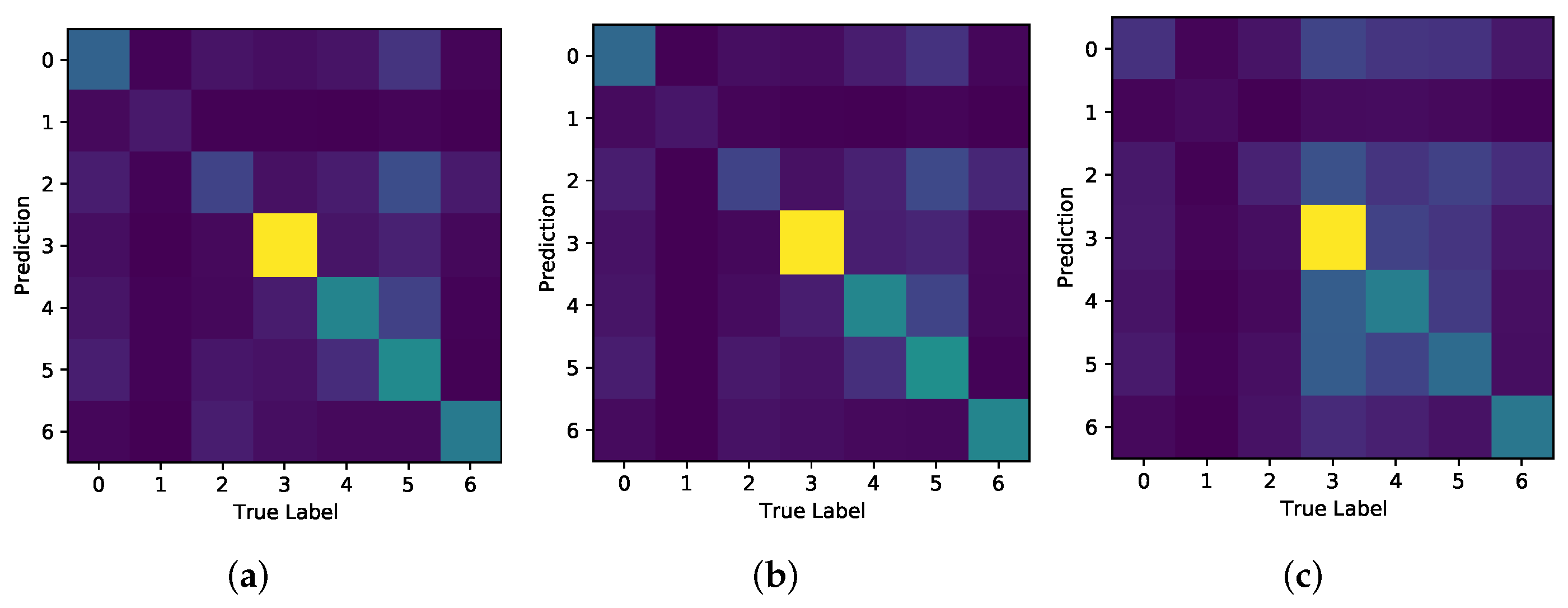
Figure 18 shows the Confusion Matrices for the experiments carried out for Model A. Each shows the strongest accuracy for true label 3, which correlates to the Joy class, of which is the dominant class. As expected, all Models struggle most with accurately classifying Disgust.

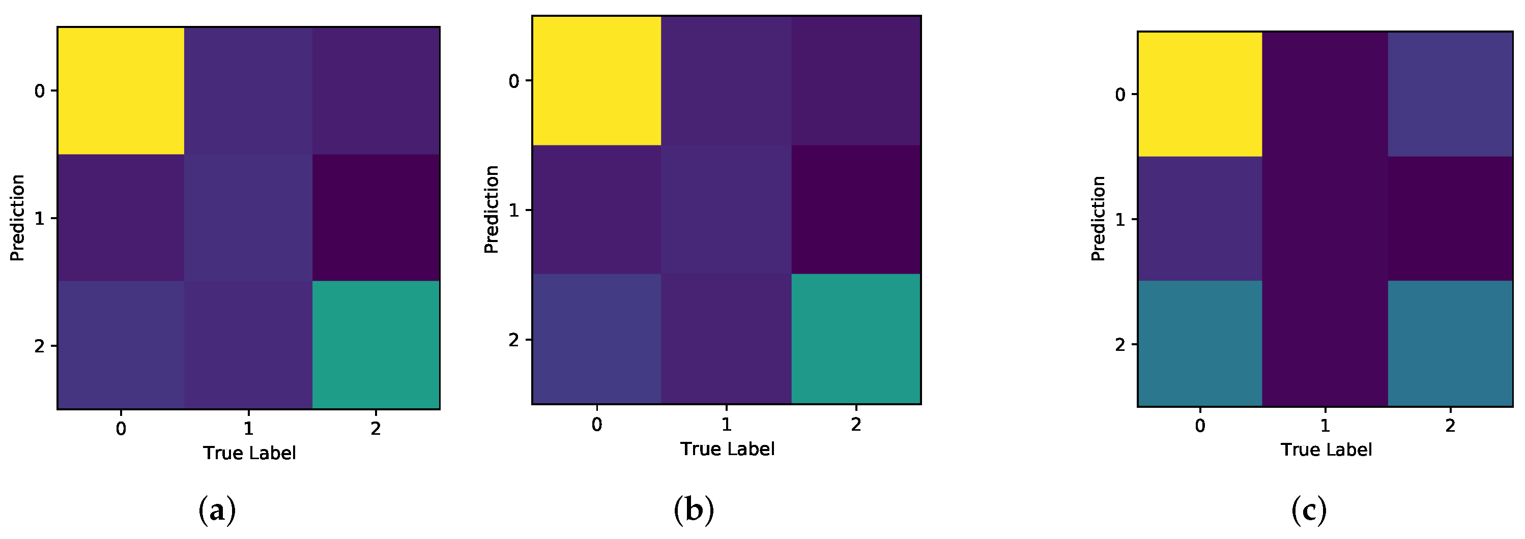
Figure 19 shows the CMs for all experiments carried out with Model B. The strongest recall for these models is in the identification of Negative; the Positive class also has a decent recall rate; however, the CM shows that the model struggles to identify Neutral on too many occasions.

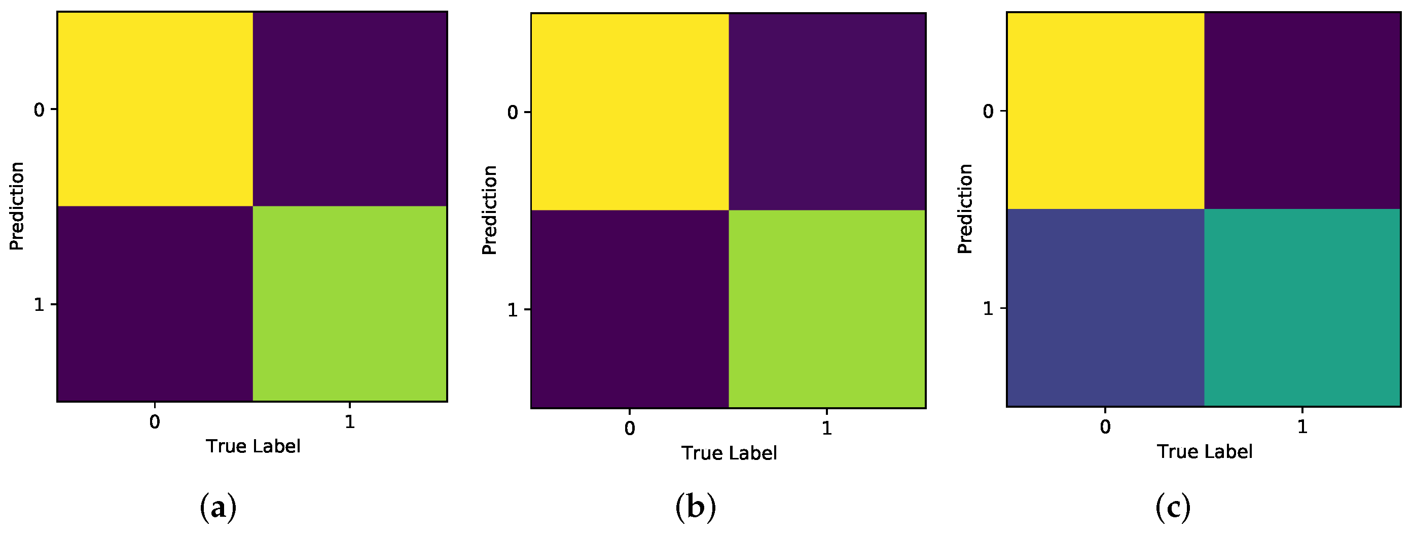
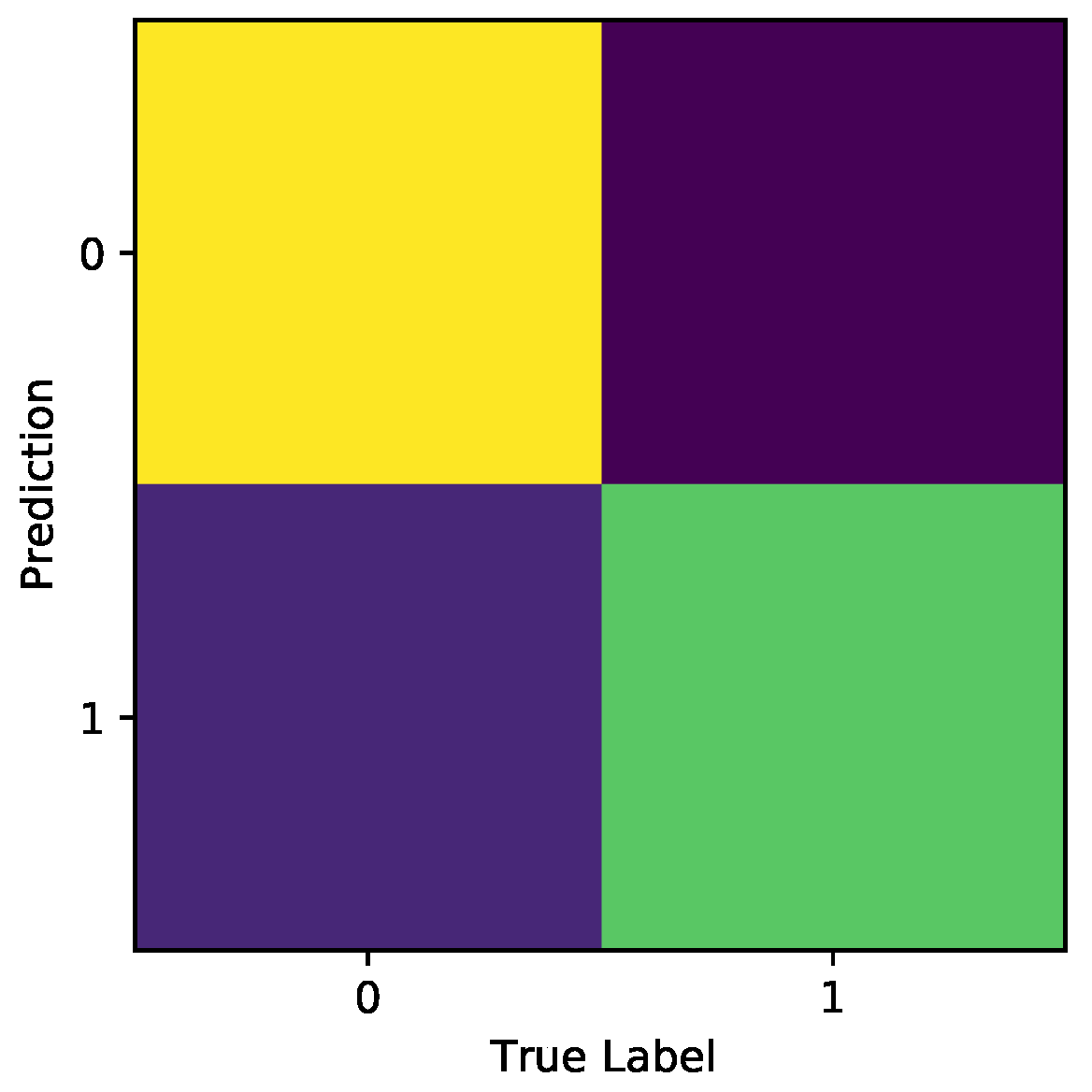
Figure 20 displays the Confusion Matrices for all experiments carried out using the binary classification data, which demonstrate the strongest performance for correct classification of Negative.

8. Model Optimisation

Deep Learning techniques are often combined with Machine Learning algorithms to improve performance. Zhang et al. [31] use a Decision Tree structure to better understand the image features that cause a CNN to classify samples into specific classes. Sun et al. [32] were able to achieve 100% accuracy in diagnosing faults with gas sensors by using a CNN with Random Forest (RF) to classify modes of signal sensors; the work concluded that methods absent of RF are inferior to this approach. This research obtains the best performance with Model C; binary classification using RGB images. This section describes how it has been optimised using Support Vector Machine (SVM). The work experimented with L1, L2 and a combination of the two regularisation techniques, consistently using a value of 0.01. Experimenting with L1, L2 regularisation during training enabled the test performance metrics to improve across the board and helped to reduce overfitting with all models.

Using L1 regularisation boosted the test accuracy for Model C experiment 1 from 79.80% to 79.91%, whilst achieving the same test loss of 0.44. Using a combination of L1 and L2 improved the test accuracy by 0.15%, maintaining the same test loss of 0.44. The greatest advantage for the model was obtained through using L2 regularisation, where the network was able to achieve 80.38% and 0.42 test accuracy and loss respectively. These results are displayed in

Table 11. Testing Accuracy and Loss After Model Optimisation.

	Train Acc (%)	Train Loss (~)	Val Acc (%)	Val Loss	Test Acc (%)	Test Loss
SVM L1	93	0.15	84.01	0.36	79.91	0.44
SVM L2	94	0.14	84.88	0.31	80.38	0.42
SVM L1,L2	92	0.19	84.19	0.35	79.95	0.44

, with the best results in bold. Refer to Figure 21 for the Confusion Matrix.

9. Classifier Deployment

This section details deployment of the classifier in more realistic scenarios. Using images that vary from the training data will develop a better understanding as to how the classifier might behave when presented with largely variable data. Secondly, deploying the classifier to predict facial expressions captured by a webcam is representational of the application. Firstly, OpenCV [33] was used to import the Haar Cascade Classifier (Viola and Jones [34]). These imports were used together to detect the region of an image containing a face and draw a bounding box around it; resize the inputs to a shape expected by the network; and to output the classifier prediction. The web framework Flask [35] was used to upload the webcam feed to an internet browser, whereby the user can see the output, the bounding box that isolates the face, and the classifiers prediction as it occurs in real-time.

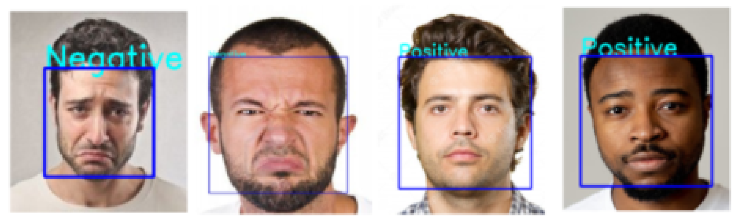
The CNN was used to classify emotions from multiple images, some showing similar characteristics, and some alternativeS to those seen in training or testing. Firstly, images that can be considered similar to those in the train and test data sets were interpreted by the model and had accurate prediction labels, see Figure 22.

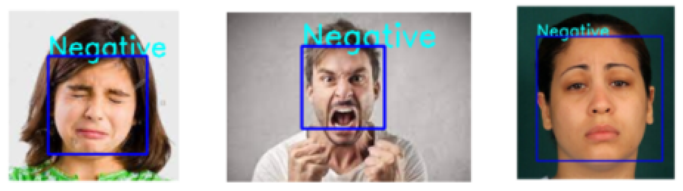
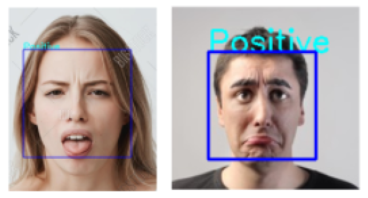
Figure 23 offers images that are somewhat different to those seen before by the model. In the first image, the person has their eyes closed; to the best of the authors knowledge, this characteristic appears infrequently in the training data. Similarly, the centre image shows negativity being expressed largely by the mouth. In the event of subtle expression, the third image conveys it perfectly, and it is accurately classified. In addition, the training data does not feature images where multiple people are expressing emotion; the model accurately predicts expressions in Figure 24.

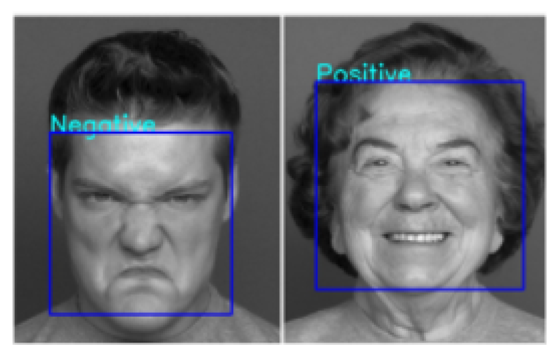
Deployed on external images caught the model inaccurately classifying expressions occasionally. Figure 25 demonstrates two examples where the predictions are incorrect, outputting Positive for samples that are showing Negative emotions.

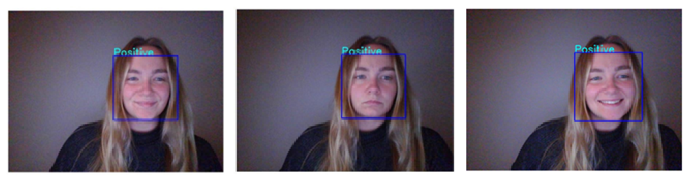
We have also tested the models working in real-time, being able to accurately classify the authors facial expressions. Figure 26 shows three variations of Positive: the first image shows a subtle smile, where most of the expression comes from the cheeks; the second image is a neutral expression, given an accurate prediction of Positive; and the third image provides a more expressive smile than the first, where the teeth are showing, and the head is slightly tilted.

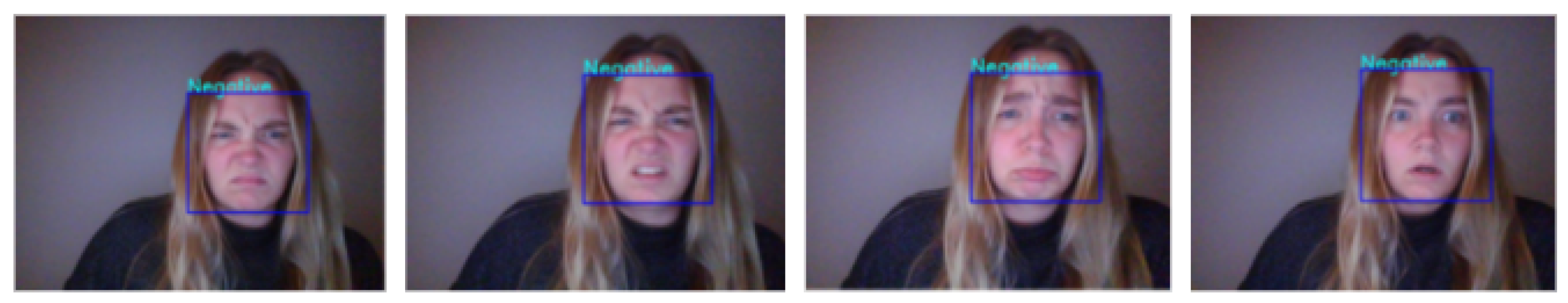
The variations of the Negative class are displayed in Figure 27: the first image shows expression of anger, the second displays disgust, the third represents sadness, the last is indicative of fear.

10. GAN

The data set used for training the Generative Adversarial Network was a collection of images displaying picturesque landscape scenery, obtained from Kaggle [36]. This is inclusive of mountains, beaches, forests, fields, lakes, rivers, deserts, and flower meadows, and was chosen due to the positive emotions the images are likely to evoke, such as relaxation and happiness, thus appropriate for the intended application area. The images are not divided into separate classes. The data used from this source totalled 536 images in RGB, all with good resolution at varying sizes, such as 682 × 1023, 1599 × 1066, 1024 × 1024. Various original samples from this data set are shown in Figure 28.

A very large number of images is required to train a generative network sufficiently; this is important to avoid image degradation, and overfitting. The small number of images obtained here is not suitable for reliable and effective image generation, however the research is constrained by hardware resources, such as limited Random Access Memory (RAM), and a singular Graphics Processing Unit (GPU). To combat this issue, Data Augmentation techniques were applied to increase the size and variability. For each original image in the dataset, a total of six transformations were performed, thus resulting in six new images for each original sample. The type of transformations are as follows:

• Rotation-Rotate images to be augmented by no more than 270 degrees
• Perspective Transform-Transform the perspective of the images using a random scale that extends between 0.0 and 0.05
• Hue and Saturation-Make additions to the hue and saturation of images with values between −20 and 20

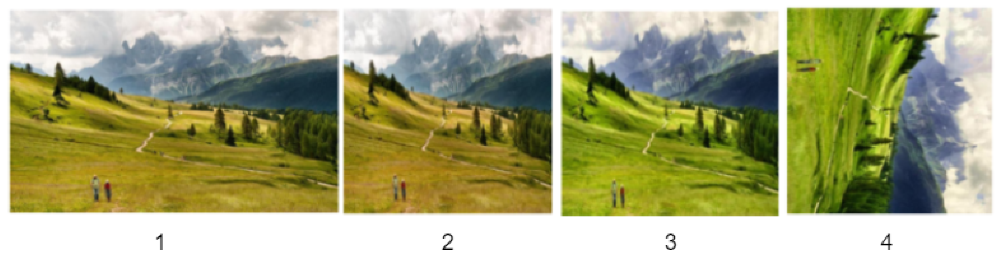
The images were also resized to 512, and the Aspect Ratio (AR) maintained with a fixed height of 600, after augmentation. This was completed so that the features in the images were preserved as much as possible. Applying Data Augmentation to the original 536 images in the data set enabled the training data to increase in size to 3752; although still a very modest size to train generative networks, this applied method is demonstrative of the simplicity involved in increasing a data set by a large amount, with minimal time and resource expenditure. Several images showing the effect are displayed in Figure 29, where the first sample is the original image, followed by three augmented versions of the same image. The top and bottom right samples are examples of adding to the hue and saturation levels in an image. This is advantageous in this particular data set because the modified images do not look unrealistic, thus expanding the number of training samples, and varying the data set, whilst not altering the realism value.

GAN Architecture: The Generator model takes a latent vector size of 150, and randomly draws points, which will become increasingly meaningful to the network as training progresses and performance is evaluated. This process is repeated until the latent dimensions represent a somewhat compressed version of the output space. PyTorch [37] was used for building the GAN, where a variety of layers can be implemented when building a Generator network to increase the realistic properties of generated images. Firstly, ConvTranspose2d is used throughout the network architecture in order to increase the area of the feature maps. The length of the latent vector is parsed in the layer, alongside the size of outputted feature maps, the size of the kernel, stride value, and padding, whilst ensuring bias is set to false so this is not learned by the network. This type of layer is often referred to as deconvolution. The number of these layers required in the generator is dependent on the specified size of generated output images. For this model, four of these layers were implemented to up sample and generate images of output size 64 × 64. A final layer of this type is required as the last block in the network where the correct dimensions for the feature maps can be parsed, for example 64 in RGB (3) format. Secondly, BatchNorm2d is a type of layer used in the Generator network so that Batch Normalisation is applied on the 4-Dimensional input and the learning rate can be managed by the internal covariate shift being minimised, as described by Ioffe and Szegedy [38]. The Rectified Linear Unit is set to true and is implemented in the network after each Batch Normalisation layer, except the last layer that uses Tanh; these activation functions are used in the Generator to aid in preventing vanishing gradient. The Discriminator network employs an architecture for binary classification, outputting a 0 or 1 for fake or real images respectively, using Sigmoid activation function. The network expects a specific input size, which corresponds to the feature map output of the Generator, in this case 64 × 64. The model uses four Conv2d layers to perform convolution over the input pixel values using kernels and stride values. Batch Normalisation is also used in the Discriminator to provide stability during training, and to encourage a faster learning pace. Leaky ReLU activation function is used throughout the network following Batch Normalisation layers, recommended for use in the Discriminator by Radford et al. [39] because of the way it promotes the smooth flow of gradients. Finally, Sigmoid activation function is used in the classifier to output a prediction.

The three main variables experimented with throughout GAN training were the latent space dimensions, the image size, and the number of epochs. Experimenting with various latent space dimensions allow for varying image realism in the generated samples. All experimentation uses image size 64 × 64 due to resource restrictions. As a baseline, a latent vector of 100 was used, and training duration was set to 1000 epochs. Output images from this configuration of parameters showed a level of pixilation and were far from realistic.

In order to develop the best performing generative models, networks are often trained for several days to output the best data. Therefore, the approach described above, where a latent space of 100 was used, the training time was doubled to reach 2000 epochs. Although these images were still far from realistic picturesque landscapes, the altered configuration offered an improvement in generated output; the images are less pixelated, more stable and are starting to resemble the target domain. Next, the latent space was altered to a value of 256, whilst maintaining 2000 iterations through the data. These generated images showed a relatively unstable output, in that several of the images look quite similar. This can indicate an approach towards mode collapse; a fatal event for the Generator output and is described by Srivastava et al. [40] as when the network becomes capable of producing characteristics of very few modes in the distribution. This is where only a singular type of output from the Generator is seen, meaning that the model has not converged.

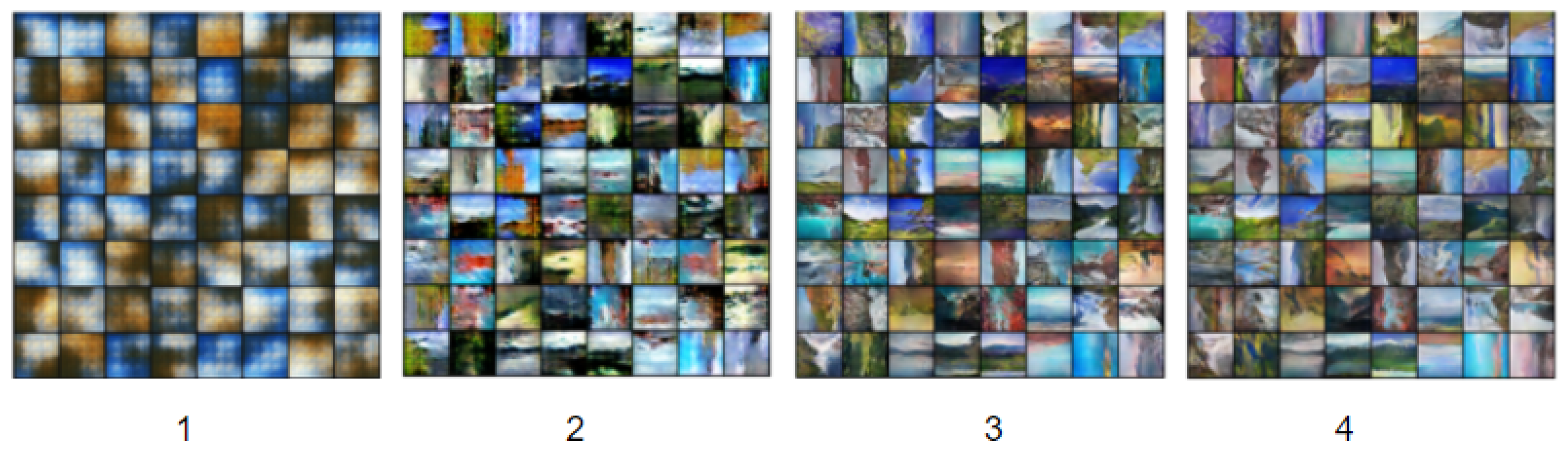
The training parameter configuration that yielded the best results utilised a latent space of 150, image size of 64 × 64, and a training duration of 2000 epochs. The progression of image generation is shown in Figure 30. From the first image to the last, a gradual improvement in generated images is shown. The first plot is very pixelated and shows only a few colours; the second plot has a better distribution of shapes across all image samples, but many samples still appear granulated; the third plot is a vast improvement compared to the previous; and the last plot shows the clearest samples thus far.

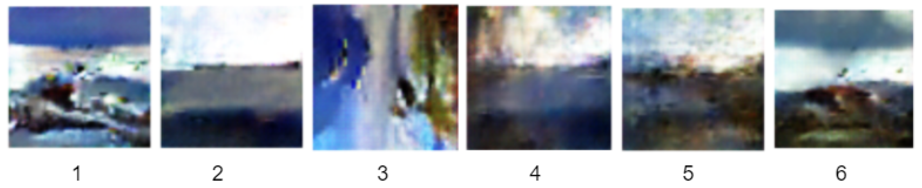
Once training has finished, the Generator model is saved alongside its’ weights to perform as a standalone generative algorithm, that will output images synthesised by the network. Figure 31 shows the example output of the trained Generator model.

The sample images shown in Figure 31 are considerably blurred, however image numbers 3 and 6 demonstrate the best output visually. The Generator outputted 64 synthesised images to a new folder, thus enabling the Frechet Inception Distance (FID) to be calculated: for the images generated the FID is 5.75.

11. Graphical User Interface

The PySimpleGUI [41] framework was used to create a simple Graphical User Interface in order to display the GAN generated images to the user if Negative expressions had been classified within the start and finish time of a pre-set timer. For example, when the webcam opens, the timer starts to count down; if negative facial expressions are classified, the GUI will appear once the timer is finished. If negative emotions are not classified in this time, the GUI will not appear. This element of the work was purposed for proof of concept only, and to spend significant time building a complex application would have deviated from the scope of research. Therefore, the resulting GUI is of limited functionality, whereby, users are able to navigate the file system, choose a parent directory, and select images that are only in .png format. The selected images appear one side of GUI, whilst the interactive file list remains on the other side. Figure 32 shows the example.

12. Discussion

This paper investigates the most appropriate type and number of classes for facial emotion recognition in the specified application domain. It experiments with varying image sizes, colour dimensionality, and Transfer Learning techniques. The same CNN architecture is used to classify images organised differently depending on the Model. The model architecture is variable by only the input size, specifically the size of images and number of colour channels. The three Models investigate the advantages to engineering a new way of looking at this task, providing that the application area is suitable. This research highlighted the difficulties in accurately classifying emotions into seven classes due to a variety of reasons. Firstly, some types of emotions expressed on the face show interference by overlapping with emotions of a different nature; the depiction between Surprise and Fear may be that the former is traditionally considered to have more positive connotations than the latter. However, the reality can be that the only difference shown between these emotions is a slight furrowing of the eyebrows. Such characteristics of emotions are also highly dependable on the individual expressing them, and any observers. Additionally, images where actors are expressing Anger compared to those expressing Disgust often have a significant level of ambiguity, where humans would also struggle to accurately classify images of this type. Supporting this, Li et al. [42] were able to conclude that the Surprise class is problematic for a classifier to predict due to its similarities to two classes, Joy and Anger. There are areas of research where it is imperative to be able to distinguish between specific emotions, such as Anger and Disgust, or Joy and Surprise. An area where this theory applies is using AI to help individuals with Autism to understand social cues that are expressed by the face. Assisting these individuals is the most advantageous to them when the information they are given is as accurate as possible. In support, Lee and Wong [43] use a combination of Computer Vision and Neural Networks to provide social assistance to individuals with Autism; as explained, the work has a significant return for the people using it, in that their social experiences can be enhanced, enabling them to maintain relationships, leading to a fuller life. Comparatively, the Models investigated in their work can be generalised to a similar application domain as the proposed. Hadfield et al. [44] use Deep Learning techniques alongside data captured by a camera to classify engagement levels of children in a classroom setting. This was developed to understand the differences in attention displayed by children described as Typically Developed (TD) and those affected by Autism. This can be expanded to consider the assessment of learning rate in children during schooling; typically, children are expressive with their faces whilst attempting to learn. This application area is an example of where the Models investigated in this paper could be applied; detecting when the learning rate of a child is halted may be understood by using binary classification: Negative or Neutral. This approach could reduce complexity where it is not necessarily required. Finally, this research contributes a combination of two AI concepts to identify negative emotion, and to aid mental-wellbeing in the immediate occurrence. To the best of the authors’ knowledge, this particular application area remains under-researched, specifically where CNNs are used to detect negative emotions from facial expressions only, and GANs are used as part of the solution. At this current time, GANs are underused in the field of improving mental well-being and reducing stress. The majority of efforts for this implementation tend towards identifying the physiological responses to negative emotions, such as a rise in cortisol levels, or an increase in sweating through the use of sensors, or EEG data. This method of data collection and participant observation is reasonably intrusive. It is also somewhat unrealistic to deploy into the workplace or a person’s home. This opens up the field of research to a more simplistic view; arguably, sometimes the best way to tell how a person is feeling is to monitor their facial expressions, and this can be done in a way that is non-intrusive. Moreover, the process of monitoring people in a physical capacity may have a negative effect on the results; wearing the technology required to capture the data may be causing somewhat of a stress response, thus causing potentially unreliable data.

13. Conclusions and Future Work

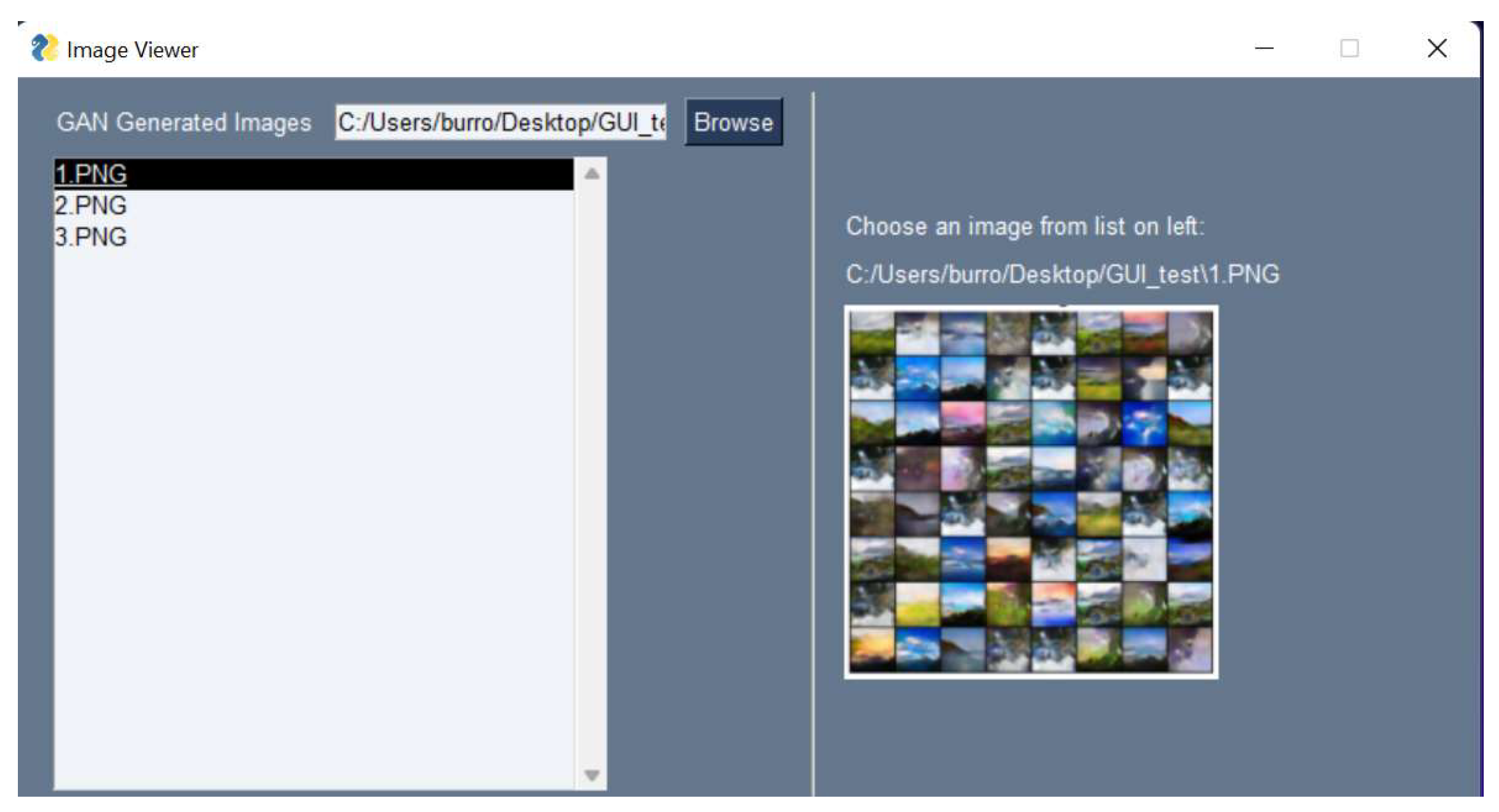
The objective of the research was to build a system capable of identifying emotions from facial expressions, and to combat negative emotions by producing media that can be argued to have a positive impact on mood. The usage of such technology would provide a form of support in the immediate time for the individual, thus potentially reducing effects felt by long-term suffering. Implementation of such a system would also contribute to highlighting the importance in taking care of mental health and could encourage people to be more outspoken about any negativity they are experiencing. The solution provided in this work is thus capable of monitoring negativity in a way that is non-intrusive; arguably this is where the research has its most importance, comparative to other works in this application area. The research was successful in accurately classifying emotions into categories that explored three varying Models. It was found that the most generalisable model implementation comes from organising the data into a binary classification problem to represent Positive and Negative emotions. The research was also successful in deploying the classifier that achieved 80.38% accuracy on unseen data, to be used in real-time, where it demonstrates a good performance. Moreover, the work is successful in image generation via a GAN, however this specific part of the implementation requires further work and optimisation in order to improve the output. Lastly, the study satisfies the objective to create a GUI to display generated media to users once negative emotions have been detected.

Taking a retrospective view of completed work is essential for improvements of the research to take place. Recommendations drawn from the assessment of this work entail using a larger data set to train the CNN in order to boost performance levels; this would be best achieved through the collection of raw data to increase the size of the training images, however, to save human efforts, this could be achieved through applying heavy Data Augmentation to existing images. Secondly, a significant amount of time needs to be dedicated to improving the performance of the GAN. This would maximise the realism of the output, thus reducing the FID score and enhancing system impact. Developing a GUI with further functionality, such as presenting the user with messages suggesting that they take a break, or listen to a piece of relaxing music, could enhance the effects of the overall application. Moreover, the research could be extended by implementation of an Intelligent User Interface, whereby the GAN obtains user-feedback in the form of positive or negative emotions captured by the CNN, thus improving output. In addition, the system could provide a log-in capability for different users, and the synthesised images displayed are dependent on their interests, such as food, or images of astronomy. This research could also navigate in an alternative direction towards a varied application area; by identifying negative emotions and attempting to reduce their effects, the possible applications for this technology are broad. For further development, the work will continue to experiment with ways that can improve accuracy and loss on unseen data. Transfer Learning will be revisited, implementing networks with a greater depth, such as ResNet50 and Xception. Furthermore, the research in its current state does not investigate the advantages of using pretrained networks to perform Feature Extraction on input data. This technique in Deep Learning often outputs SOTA results for tasks such as this. Further research will also entail improving the data used for the CNN and GAN. More specifically, a more detailed and in-depth performance of the CNN could be obtained if the work were to use cross-database testing, whereby the test data set consists of images different entirely to the ones used in training. Regarding the GAN, training time will be increased dramatically after vast experimentation with parameter tuning. This application area has a lot of potential due to the magnitude of prospective benefits from successful and reliable techniques. For example, once a well-established model with competitive performance has been developed, the work could navigate towards other forms of identifying stress, such as using sensors in chairs used at work to detect levels of restlessness, and heavy breathing. Moreover, the GUI presented here could be extended in functionality significantly. For example, an escalation system could be introduced, where if a small number of negative emotions are detected in a twenty-minute period, subtle messages appear to the user first, such as “have a coffee break”. After this condition has been met and negative emotions are still detected, the GAN images are shown to the user.