IPDCA: Intelligent Proficient Data Collection Approach for IoT-Enabled Wireless Sensor Networks in Smart Environments

Abstract

The Internet of Things (IoT) enables the interrelation of physical things and devices that can be accessed through the internet and it simply forms a single integrated network of various things. An IoT-facilitated smart city scenario spans several sectors, such as industrial applications, public transportation, smart grid, emergency services, health care, etc. In this paper, we propose an Intelligent Proficient Data Collection Approach (IPDCA) to deliver public data in a large-scale smart city set-up. IPDCA utilizes public vehicles as the mobile data collectors (D-collectors) that read (or collect) data from multiple Access Points (APs) and send them back to the central Base Station (BS). Moreover, IPDCA adopts a modified Bat algorithm for path finding of D-collectors, where we extend the Bat algorithm to solve our discrete optimization problem. Besides, for selecting D-collectors in smart city settings, we use a multi-objective fitness function that considers the count, travelled distance, and storage of D-collectors to ensure optimal use of resources. Efficiency of the proposed mechanism is proved through simulations.

1. Introduction

Nowadays, smart homes, smart devices, and several other smart systems are becoming ever more popular. The general view of these systems is focused on a single concept, known as IoT [1]. An IoT system can be ‘whatever’ that contains the technical components, which allow the thing to link to the Internet through a wireless or wired network. The users of the IoT can be a person, a machine, or a combination of both [2]. The vision of the IoT seeks to incorporate the sensing and actuation characteristics in everyday objects seamlessly by leveraging their network capacities to create pervasive information systems [3,4,5]. Wireless Sensor Network (WSN) is often a technology used within an IoT system that supports multi-user access through a multi-application platform, and smart city is an example of such type of system.

Smart City is a modern way of thinking about urban space, incorporating Renewable Energy Sources and Systems (RESSs), energy conservation, sustainable mobility, environmental security, and economic growth, which reflect the priorities for future developments [6,7]. Users in a smart city may be interested to use (1) smart grid information, (2) availability of parking space [8], (3) details regarding smart tourism [9], (4) Accessing medical information [9], (5) Major road accidents in the city etc.

The IoT helps smart cities to connect and manage multiple infrastructure and public services. From smart lighting and road traffic to networked public transport and waste disposal, the range of applications is very diverse. What they have in common are the results. Applying IoT solutions leads to lower energy costs, optimized use of natural resources, safer cities and a healthier environment. Example of these applications includes: Smart traffic solutions in the smart city use different types of sensors and retrieve GPS data from drivers’ smartphones to determine the number, location and speed of vehicles. At the same time, smart traffic lights connected to a cloud management platform can monitor green light times and automatically switch lights according to the current traffic situation to avoid traffic jams. Additionally, by using historical data, smart traffic management solutions can predict where traffic might go and take action to avoid potential traffic jams. With the help of GPS data from driver smart phones (or road surface sensors embedded in floor areas of parking lots), intelligent parking solutions determine whether parking spaces are occupied or available, and create a map parking space in real-time. When the next parking space becomes available, drivers will receive a notification and use the map on their phone to find a parking space faster and easier instead of driving blindly. IoT smart city solutions can also provide public service management services to citizens. With these services, citizens can use their smart meters to remotely monitor and control their usage. For example, a head of household can turn off his central heating using a cell phone. Additionally, if a problem arises (such as a water leak), utilities can notify households and send specialists to fix the problem. Smart cities based on IoT make the maintenance and control of street lights easier and cheaper. By equipping the street lamps with sensors and connecting them to a cloud management solution, the lighting program can be adapted to the lighting area. IoT-enabled smart city solutions help optimize waste collection plans by tracking waste quantities and providing route optimization and operational analysis. To improve public safety, IoT-based smart city technologies offer real-time monitoring, analysis and decision-making aids. By combining and analyzing data from acoustic sensors and CCTV cameras deployed across the city with data from social media, public safety solutions can predict potential crime scenes. In this way, the police can successfully arrest or track down potential perpetrators.

An example of a Smart City application is Barcelona, one of the main cities in Spain, which is using sensors to help monitor and manage traffic, also deployed a smart parking system. Further, the city uses smart LED street lamps. Moreover, the city is using sensor technology to enhance irrigation efficiency, which is critical when drought occurs. These sensors monitor rain and humidity to determine the quantity of water needed to irrigate parks [10].

In order to provide large-scale access to information, smart cities are required to incorporate a multitude of wireless networks and architectures. Pervasive sensing (PS) is an especially promising model in this regard. The principle of pervasive computing is to equip some kind of computing facility with commonly used everyday items. PS enables low-power, tiny, and smart objects to evaluate the sensed data and send the processed data to the designated sink, wherever that may be [11]. Under the IoT framework, PS will be extended to incorporate schemes for generating and sharing heterogeneous data in smart cities, which includes WSNs, personal and environmental monitoring devices, and database centers that are deployed in both urban and rural areas.

So, IoT-enabled WSNs can be used to enhance the standard of smart city living and the residential experience [5]. In such environments, sensors are widespread and accessible to people, and they are integrated with public or private vehicles, and (or) installed on buildings and roads. To ensure better and cost-effective data distribution in such a wide-range PS model, an effective data sharing or delivery mechanism must be used in the sensing phase. There are many research work introduced in this field to address data delivery using Mobile Data Collector (D-collectors) [12,13,14,15,16]. It is proven that networks with Mobile D-collectors use less energy than networks with static D-collectors [17] and thereby it enhances the network lifetime. In this work, to provide efficient data collection in the network, we are employing multiple Mobile Data Collectors (D-collectors). We have to consider latency, energy use, and the available storage capacity of the D-collectors in the system in order to provide an effective path-planning of D-collectors. The optimal path planning of these mobile D-collectors is considered to be very challenging in an IoT environment and which is addressed in many works, e.g., [18,19]. In [19] authors addressed the Mobile D-collectors’ Cognitive Path Planning in a precision agriculture wireless sensor network. Whereas in [18], authors addressed the same using a hybrid collaborative method by combining a Genetic algorithm and an improved local search approach in an IoT environment.

Figure 1 reflects our smart city scenario, which consists of multiple users on the same platform with multiple applications. The smart city model depicted in Figure 1, contains a two-tier telecommunication framework. In the bottom tier, it comprises of sensor devices or nodes (SN) that sense its surroundings and transmit the sensed data towards Access Points (APs) in the network. To save energy, these sensor nodes often have fixed and restricted transmission ranges, and do not relay traffic. APs in the top layer gather and deliver the data from SN to the D-collector present in their communication range. Finally, each D-collector delivers the collected data to the Base Station (BS) or sink. APs and D-collectors present in the top tier possess better transmission range and they communicate with the BS periodically to deliver the collected data from the bottom tier. An example scenario of data gathering using D-collectors in a smart city is illustrated in Figure 2. According to this figure, there are 10 APs and a minimum number of D-collectors (three D-collectors here) to serve these APs.

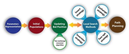
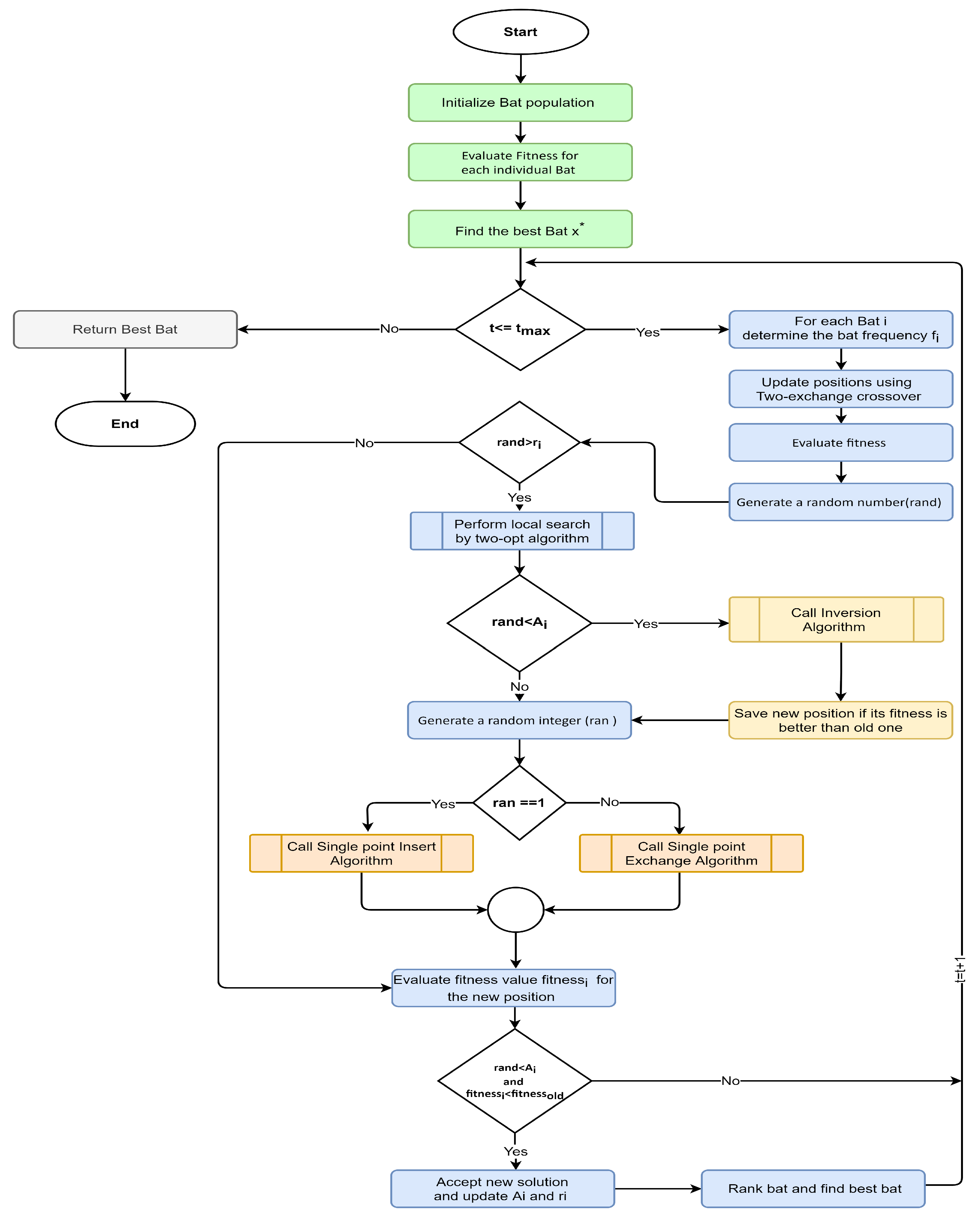
In this work, our focus is on the path planning of mobile D-collectors utilizing a nature-inspired meta-heuristic algorithm named Bat algorithm that minimizes the required number of D-collectors and their respective travel distances in a smart city scenario. We propose and utilize Bat algorithm-based D-collector path planning (BDPP) to provide a solution to this multi-objective problem. Our contributions are summarized below:

• For Mobile D-collectors in smart cities, we propose a massive data collection framework. We accomplish this by employing moving sensors that efficiently collect data in a smart environment in terms of both the number of D-collectors engaged and the total distance covered by each D-collector.
• We propose a Bat algorithm-based pathfinding solution for D-collectors (BDPP) that operate in competitive time complexities and satisfy the traffic and memory power constraints.
• We also introduce a cost-based fitness function in the pervasive sensing model for the election of D-collectors, and we consider the resource limitations of D-collectors in different aspects that include count, energy consumption, throughput and storage capabilities.
• We compared our BDPP approach against other heuristic-based schemes (e.g., HS, EF, and, HCPF).

The rest of this paper is arranged as follows: Section 2 reviews the related research works. Section 3 sets out the system models and the description of the problem. Section 4 explains our approach in detail. Section 5 describes an example scenario. Section 6 gives the details about the simulation, and finally Section 7 concludes our work.

2. Related Work

One of the fundamental or atomic components of IoT is WSNs [4,5,20,21,22,23,24,25] and IoT data acquisition requires a WSN. In an integrated urban development, WSNs play an important role and are vital for smart cities. WSNs can be used in smart cities in a variety of applications and these applications include parking optimization, road traffic management, environmental monitoring, city security services [26], home and office automation solutions (HOS) [27], and energy monitoring in smart grids [28] etc.

A WSN is typically made up of tiny and low-powered sensor devices that can perceive, process, and interact with each other through wireless communication. The sensor devices have constrained memory, computing power and battery capacity. They gather and deliver data to a BS through mobile D-collectors for data’s further processing by IoT systems. To gather accurate data from sensors, it is important to use a number of mobile D-collectors and effectively use their path of interest. The D-collectors are often low-powered devices integrated on a mobile vehicle (e.g., public vehicle). Thus, the D-collectors in the formed networks are assumed to have limited energy, memory, and computational power. As a result, connecting a secure smart city wireless network to the central BS is challenging. This section mainly introduces some previous research related to our work.

The application of mobile D-collectors for WSN data collection is a common practice for improving the network lifetime, reducing the latency incurred during the transmission [29,30,31] and improving network coverage [32].

Mobile sink (MS) is adopted as a mobile data collector in performing an effective collection of sensor data in several works, e.g., [33,34,35]. A distributed method, called GTAC-DG (Game Theory and Ant Colony Data Gathering) [34] takes the benefit of game theory along with ant colony optimization as a swarm intelligence method to select the best path for the MS. The work in [33] utilizes a network flow approach for data collection, where, fixed-path mobile sink is mapped to a network flow optimization issue. In their work, a data forwarding algorithm was developed for data collection using MS(s) for a path-constrained environment. Best visiting points for mobile sink among clusters are considered in [35]. Modified Travelling Path Algorithm (MTPA) is proposed in [34] for data gathering in WSN. MTPA is developed to find the shortest traveling path for the mobile sink.

In [36], the data collection trajectory of MS is optimized using the Hilbert curve. The network field is divided into clusters, then, for each cluster, a VRP (virtual rendezvous point) is chosen for the MS to visit based on an integer linear program considering optimal communication range between the sensor node and sink.

A three-tier communication-based approach called Fuzzy Logic-based Effective Clustering (FLEC) was proposed in [37]. In FLEC, data is sent from sensor nodes to cluster-heads (CHs), then to super CHs, and finally to MS. FLEC considers mobile BS that uses a model based on the random way-point mobility in the network without using any path determination method. A mobile data collector (MDC) is employed in [38] to restore network connectivity. The MDC regularly visits and collects data from partitions. Moreover, the Steiner zone approach is utilized to designate respective data collection points for corresponding partitions.

In [39], a mobile data collector is employed to act as a broker between WSN nodes and BS, where, the network is divided into four logical partitions and the MDC utilizes a learning automata (LA) to proceed towards the area center or to the network center at regular intervals of time. Based on the learning automaton, updates the best logical partition at each interval selected by the mobile collector. A collaboration between multiple mobile robots and WSNs is adopted in [40]. Sensor data are routed through mobile robots equipped with a mobile sensor node to a BS.

In [41], the network is split into sub-clusters based on fuzzy logic, after constructing a Minimum Spanning Tree. Then, cluster heads are chosen based on the number of hops to the root of the tree, the density, the residual energy of nodes, the number of packets to forward, and the node’s centrality. Mobile data collectors begin their trajectory starting from the head node and return to the BS covering the subset of suitable CHs in accordance with their positions.

In [42], the authors proposed a new approach for optimizing the mobile D-collector path to balance the latency and energy consumption in data collection using a modified Genetic Algorithm (GA). This approach uses a single D-collector for visiting all the nodes in the network and chooses a path that has reduced total path length. Authors in [43] present rendezvous-based delay-constrained data collecting solutions for WSNs using multiple Mobile Elements (MEs). The proposed methods enhance WSN lifetime utilizing MEs tours planned through higher energy areas of the network and also areas where greater energy consumption has been noticed. By deriving MEs tours that pass through energy-rich areas of the network, as well as regions where increased energy usage has been observed, are used in the proposed approaches to extend network lifetime. A method of data collection based on data volume utilizing MDC was introduced in [44]. In the proposed technique, MDC moves only to the nodes that produced data while ignoring the remaining nodes in the network.

A lot of studies have focussed on data collection in IoT. In [45], software architecture is introduced to support the IoT data collection. By processing enormous datasets collected from physical nodes, the architecture supports Big Data analysis. In [46] authors proposed a data collection algorithm in IoT. During data collection, the proposed algorithm was designed to maximize throughput and reduce traffic congestion. To provide data-centric universal data gathering of hypermedia Big Data in IoT, authors proposed a distributed algorithm named EQRoute in [47].

In [48], a mobile data collection approach based on adaptive dual mode routing, called ADRMDGA, is proposed for IoT-based Rechargeable WSNs (RWSNs). In ADRMDGA, a mobile charging vehicle is in charge of performing data collection, and a dual-mode approach is adopted for data routing to balance the energy utilization.

In our work, we address the path planning problem of the mobile D-collectors. One of the most widely adopted methods in this category is a potential field approach [49,50] where attractive force towards the target and repulsion by the obstacles are checked to assess the ability to direct the D-collector towards the target. However, this strategy faces the problem of local minimum. Other approaches like probabilistic road map [51,52] works through random points generation and collision avoidance check for obstacles, or rapidly expanded random tree [53] where branches of the tree extended in various directions and are connected to others to produce the route. Other approaches include the use of intelligent route planning schemes [54,55]. Although these methods are effective, these solutions cannot be applied in the smart city set-up that requires us to satisfy the constraints of different D-collectors.

There are genetic-based meta-heuristic solutions for various IoT services, including the Hybrid search (HS), Effective Fitness (EF) and HCPF algorithms [18,56,57]. The movement direction of the mobile carrier is considered by EF with certain environmental effects, such as surrounding barriers and paths available to be used with the genetic algorithm. However, HS is a modified and more effective approach that considers the speed of motion while determining the fitness value. In HCPF a hybrid approach of genetic algorithm and improved local search is used to find the path of D-collectors. The work in [58] investigates an emerging technology known as LoRaWAN (Long Range Wide Area Network) and claims to the current best choice for the major IoT scenario, which includes smart grids. LoRaWAN is a truly convergent, low-cost technology built from the ground up to create urban IoT platforms. The authors in [58] address the issue of data delivery between smart grid meters using LoRaWAN. For a comprehensive analysis, we have taken a genetic algorithm with HS [57] and EF [56], data delivery between smart grid meters using LoRaWAN [58], and HCPF [18] to compare the data delivery approach in a smart city scenario. Unfortunately, in some of the above-mentioned collaborative methods, certain criteria such as the total traversed distances, and the current application conditions were not taken into account. Our approach, on the other hand, takes into account D-collectors and different environmental constraints and, as a result, can be applied to manage more challenging environments with various constraints. We also provide a comprehensive framework that addresses multiple challenges that include cost, resource management, and delivery simultaneously.

3. System Model

Smart cities enhance the efficiency of various city operations, including security, tourism, transportation, etc. through a data-driven decision-making process. This phenomenon needs a continuous collection of information from sensors deployed across the city [59]. To ensure data collection from sensors spread across the city, this paper presents mobile data collection schemes focusing on the use of a minimum number of D-collectors with minimum traveled distance satisfying different smart city constraints. In the following, we discuss the problem statement and constraints, network model, and energy and communication model of our approach.

3.1. Problem Statement and Constraints

In a smart city, we practice handling multiple users with different attributes, such as throughput, reliability, and latency, simultaneously. This is a critical area that has not received sufficient research consideration. The major challenge in managing the heterogeneous flow of traffic in the underlying sensor networks arises from the simultaneous processing of user requests with varying requirements. To address this challenging issue, we suggest an approach that uses smart mobile devices known as Mobile D-collectors. To reduce the total number of D-collectors and their total traveled distances, we propose an algorithm called BAT Algorithm based D-collector Path Planning (BDPP).

We state the problem as: Given a set of D-collectors with limited storage and predefined trajectories in the coverage of a set of APs, determine the least number of D-collectors that can transfer data traffic of these Access Points (APs) while maintaining storage capacity limitations and D-collectors short travel distance.

The scenario above can be seen in a smart city network, i.e., data gathered by smart city sensors is sent to the access point (AP), and the AP needs to send this data to the BS. To efficiently utilize the APs’ resources (e.g., energy), a public vehicle (e.g., taxi, transport bus) will be used as a mobile D-collectors with a fixed storage capacity to transmit this data to the BS. There are numerous public vehicles available throughout the city for this purpose. Our goal is to efficiently select the optimal number of such public transport vehicles with minimum travel distance.

In our model, we consider the following inputs:

• All the D-collectors are identical and have specific or limited storage capacity
• Each access point has a specific traffic load to deliver to a D-collector

Following describes the constraints used in our work:

• Each D-collector is associated with exactly one route.
• Set of routes (or one route) forms a path and that path may cover all APs in the network. A route contains a subset of APs.
• Each AP should be assigned to one D-collector (visited once).
• Sum of traffic loads of all APs in a route of a D-collector cannot be more than the storage capacity of that D-collector.

3.2. Network Model

In this work, a two-tier telecommunication framework is considered [60], which consists of three components: BS, Mobile D-collectors and Access point (AP) (in Figure 1). In the bottom layer, it includes the sensor nodes (SN) that sense their surroundings and transmit the sensed data towards APs in the network. To save energy, these sensor nodes usually possess fixed and restricted transmission ranges and they do not relay traffic [18]. APs in the top tier gather the data from the SN and deliver it to the D-collector present in their communication range. APs and D-collectors present in the top tier have a longer transmission range and connect with the BS on a regular basis to hand over the collected data from the bottom-tier. Each D-collector will start and end in the BS, and is equipped with wireless transceivers. In addition, at the top of our specific architecture, we determine the size of the data packets as well as the order of the targeted intermediate nodes, each of which has a load that must be transmitted to the BS. A data packet contains data traffic from a group of APs in the network. Each AP transmits its sensed data to BS via other APs/D-collector in a multi-hop fashion. D-collectors are in charge of delivering data loads from APs to the destination (BS or AP) once they reach its communication range.

3.3. Energy and Communication Model

The mobile D-collectors energy supply can either be restricted or unlimited. When a D-collector has an unlimited energy supply (rechargeable or simply sufficient energy with respect to the APs’ expected lifetime), D-collector placement is to provide access to a limited range of APs that meet the constraints. If D-collectors have limited energy supply, the D-collectors selection is done such that it ensures the connectivity of the APs and guarantees that the path of the D-collector towards the BS is constructed without any violation of energy limits. In this work, we assume that the power supply for D-collectors a limited and fixed.

The energy consumption model used is similar to [61], and described as follows:

$$E_T^r(r,b)=b\ast (e_{elec}+e_{amp}\ast r^{\gamma }).$$

(1)

$$E_R^r\left(b\right)=b\ast e_{elec}.$$

(2)

where $E_T^r(r,b)$ and $E_R^r\left(b\right))$ are the transmission and reception energy for b bits to a distance r, respectively. $e_{elec}$ is the electronics energy, $e_{amp}$ is the amplifier energy and $\gamma$ is the path-loss exponent. According to [61], values of r is 50 m, $e_{elec}$ is 50 nJ/bit, $e_{amp}$ is 0.1 nJ/bit/m², $\gamma$ is 2. So energy consumed in a round j by a sensor node can be written as

$$E_{cons}^j=\sum E_T^r(r,b)+\sum E_R^r\left(b\right).$$

(3)

If $E_{init}$ represents the node’s initial energy at the start of a round, then the energy at the end of the round can be computed as, $E_{rem}^j=E_{init}^j-E_{cons}^j$. Based on [62], the total consumed energy of D-collector to receive the packet is

$$E_{D-collector}=(x\ast ((P_r\ast L_d)/R_d))+y(P_t+\left(P_{D-collector,SN)}\right)/k)\ast L_a/R_a,$$

(4)

where $P_r$ and $P_t$ are the power needed to run the processing circuit of the receiver and the transmitter. $L_d$ and $L_a$ represents the size of data packet sent from SN to D-collector and size of the acknowledgement, and $R_d$ and $R_a$ are the respective data rates, $P_{D-collector,SN}$ is the transmission power, k is the power amplifier efficiency and y and x values are based on the forward and backward link reliability respectively.

We follow the same communication model in [18], which is given as follows: According to the log-normal shadowing model, the signal level at a distance d from the transmitter follows a log-normal distribution centered on the average value of power at that point. We can represent it as,

$$P_r=K_0-10\gamma log\left(d\right)-\mu d.$$

(5)

In Equation (5), d is the Euclidean distance from the transmitter to receiver, $\mu$ is the random variable indicating the signal attenuation effect, $\gamma$ represents the path loss exponent, and $K_0$ is a constant computed according to the receiver, transmitter, and field mean heights. Let the value of $P_r$ represents the minimum acceptable signal level to keep the connectivity. Based on a probabilistic model of communication, the probability that two devices located d distance apart will be able to communicate is calculated as follows:

$$P_c(d,\mu )=K{e}^{-\mu d^{\gamma }},$$

(6)

where $K_0$ = 10 log (K). Thus, the connectivity probability given by $P_c$ is not only a function of the distance but also of the surrounding terrain and obstacles, which can induce multipath and shadowing effects (portrayed by $\mu$) [18]. The values of these parameters are taken from [18].

4. IPDCA: Intelligent Proficient Data Collection Approach

In this section, we discuss our proposed IPDCA approach for intelligent data collection. IPDCA employs Bat Algorithm (BA) as a swarm-intelligence algorithm and modifies it to present a new algorithm called BAT Algorithm based D-collector Path Planning (BDPP) for improving the path-finding in smart cities with respect to application-specific characteristics, such as bandwidth availability and delay-sensitivity. First, we provide background on the Bat algorithm. Then, we present our BAT Algorithm based D-collector Path Planning (BDPP). BDPP algorithm saves the original concept of the basic BA algorithm, but we modified BA to support our approach.

4.1. BAT Inspired Algorithm Background

BA is a meta-heuristic search algorithm introduced by Yang in 2010 [63] that mimics the echolocation behaviour of bats to identify the prey and differentiate between different types of insects with differing pulse emission and loudness rates even in complete darkness. The algorithm contains N bats (population), representing solutions. At various generations t, these bats fly in a D-dimensional search domain, modifying their positions $x_i^t$ and velocities $v_i^t$ based on the following three equations [63]:

$$f_i=f_{mn}+{\beta }_1(f_{mx}-f_{mn}).$$

(7)

$$v_i^t=v_i^{t-1}+f_i(x_i^t-x^{\ast }).$$

(8)

$$x_i^t=x_i^{t-1}+v_i^t,$$

(9)

where $f_i$ is the frequency and $f_i\in [f_{mn},f_{mx}]$ and the value of $f_{mn}$ and $f_{mx}$ are the problem-specific parameters, ${\beta }_1$ represents random number vector drawn from uniform distribution 0 and 1. The $x^{\ast }$ variable denotes the current best global position (solution) after all the solutions given by the m bats have been compared. A bat is associated with a fitness function $f\left(x_i\right)$. Each bat has loudness $A_i^t$ and pulse emission rate $r_i^t$. A local search is carried out with a probability $r_i^t$ around the current best solution (global), resulting in a new solution for every bat using a random motion, which can be represented as,

$$x_{new}=x_{old}+ϵA^t.$$

(10)

where, $ϵ\in [-1,1]$, and $A^t$ is the bats average loudness at generation t. A better value for the fitness function $f\left(x_i\right)$ leads to increasing the rate of pulse emission and decreasing a bats loudness, therefore, $A_i^t$ and $r_i^t$ will be updated using

$$A_i^{t+1}=\alpha .A_i^t,r_i^{t+1}=r_i^0.[1-exp(-\Gamma .t)]$$

(11)

where $\alpha$ and $\Gamma$ are constants.

Steps involved in the classic bat algorithm are given below:

• Initialize bat population: initialize position ($x_i$), velocity ($v_i$) and frequency ($f_i$). The virtual bats movement is provided by their velocity and position updates $v_i^t$ and $x_i^t$ at time step (t) respectively, using Equations (7)–(9).
• A random number $rand$ is applied.
  • If $(rand>r_i)$, then select a solution from current best bat solutions,
  • Then, a new solution will be generated around the current best solutions; it is expressed by Equation (10).
• Update the loudness ($A_i$) and the $r_i$ (pulse emission rate), and a solution will be accepted if $rand$ is less than $A_i$ and $f\left(x_i\right)<f\left(x^{\ast }\right)$. Update $A_i$ and $r_i$ using Equation (11).
• Repeat the steps until maximal iterations count is reached.

4.2. BAT Algorithm Based D-Collector Path Planning (BDPP)

The BA was basically created to optimize continuous non-linear functions [63,64] in which each bat moves to a continuous-valued location in the search space, however, several problems are characterized by discrete-valued spaces having variables’ domain as finite. In this paper, BA is discretized to solve the D- Collector path planning problem. The following subsections explain the various steps taken to solve D- Collector path planning by expanding BA’s version. The flowchart of the proposed BDPP approach is given in Figure 3.

4.2.1. Parameters Representation

In this study, position, velocity, and frequency of a bat are represented as follows.

• The solution of n APs determined by the $ith$ bat is defined as, $x_i=(x_{i1},x_{i2},\dots ,x_{in})$ an n-dimensional vector.
• The velocity $v_i$ is presented as a permutation set ${\pi }_i=\{c_1,c_2,\dots ,c_n\}$, which helps to be near to the global best solution, given by $x^{\ast }=(x_1^{\ast },x_2^{\ast },\dots ,x_n^{\ast })$.
• In the frequency range $[f_{mn},f_{mx}]$, each bat selects a frequency $f_i$, where $f_{mn}$ and $f_{mx}$ are two integers ∈$[1,n]$, where n is the APs count. $f_i$ indicates the APs count saved from the current solution $x_i^t$.

The following example will clear this representation. In this work, the word ‘path’ represents the solution of the problem or simply a set of routes found by the BS to serve all the APs in the network, and the word ‘route’ represents the path of a single D-collector (which is clearly explained in the following example).

Example 1: Every solution (Path) is illustrated as a unique sequence of route, separated by 0, where 0 represent BS and count of zeros represents the count of D-collectors required. An example scenario of a 10 APs and 3 D-collectors are shown in Figure 2. The path sequence of this scenario is represented as:

Solution (path): [0; 1; 10; 5; 0; 3; 4; 2; 6; 0; 9; 7; 8]

Route 1: BS 1 10 5

Route 2: BS 3 4 2 6

Route 3: BS 9 7 8  

These are the routes found for the three D-collectors used in this example by the BS. So the first D-collector travel from BS → AP1 → AP10 → AP5 → BS. Second D-collector travel from BS → AP3 → AP4 → AP2 → AP6 → BS. The third D-collector travel from BS → AP9 → AP7 → AP8 → BS.

In the above example we can represent the position of a bat as x = [1,10,5,3,4,2,6,9,7,8]. We will use these position representations in the two-exchange crossover algorithm (which is explained in Section 4.2.3) to generate the new position.

4.2.2. Initial Populations

The strategy for developing an initial bat population plays an important role in the algorithm. In this step, we select the nearest nodes to a particular node to generate the location sequence. The purpose is to decide each node’s nearby nodes and prevent it from being fully random while generating an initial population of bats. This data is collected over many communication rounds and contributes to a D-collectors knowledge Base (KB) that can be analyzed by reasoning processes to make quick decisions about the sub-path of data delivery. We use a quality-aware cognitive routing (QCR) algorithm in [18] for generating KB at the D-collectors.

4.2.3. Updating Bat Position

For updating the bat position in continuous BA, Equations (7)–(9) are used. Using Equations (7) and (8), the bat’s velocity value is updated, and the obtained value is applied to Equation (9) for updating each bat position. We cannot apply these equations directly in our problem for updating the position of bats and we need to adjust them to solve our problem.

Similar to standard BA, in the frequency range $[f_{mn},f_{mx}]$, each bat selects a frequency $f_i$, where $f_{mn}$ and $f_{mx}$ are two integers ∈$[1,n]$, where n denotes the APs count. The value of frequency $f_i$ indicates the count of APs saved from the current solution $x_i^t$.

By using the two-exchange crossover [65] we will cross current solution $x_i^t$ and current best solution $x^{\ast t}$(both current solution and best solution represented by the position representation from Example in Section 4.2.1) and generate the velocity $v_i^t$, which consists of a set of permutation.

The following example will illustrate the idea of the two-exchange crossover algorithm. In this example (see Figure 4), we set the frequency value as 3 and the cost matrix C, which is defined as follows.

$$C=\left(\begin{array}{ccccccccc}0& 9& .& 6& 7& 3& 5& 2& 4\\ .& 0& 4& 6& 4& 8& 11& 10& 8\\ .& 3& 0& 10& 12& .& 7& 5& 4\\ 5& 7& 9& 0& 3& 5& .& .& 16\\ 6& 5& 10& .& 0& 8& .& 15& 11\\ 2& 9& 5& .& 6& 0& 8& 5& 7\\ 6& 10& 9& 6& 11& 7& 0& 2& 3\\ 3& 9& 6& 4& .& 4& 3& 0& 2\\ 5& 7& 4& 12& 10& .& 3& 3& 0\end{array}\right)$$

Considering two solutions $x_1$ and $x_2$, we will cross these solutions to get a new solution (Figure 4) $x_{new}$. At the beginning of the two-exchange crossover, we save the first f, APs from solution $x_1$ and mark this as already assigned in $x_2$. The new solution $x_{new}$ is initialized by the APs saved from $x_1$. Next, continue to append the last AP of $x_{new}$ by the nearest AP from either $x_1$ or $x_2$. While generating the new solution, it must guarantee that AP was chosen from solution $x_1$ and solution $x_2$ is not already marked in $x_{new}$.

4.2.4. Local Search Methods

The concept of a local search or a neighborhood is essential for combinatorial problems and also for continuous problems [66]. Local search techniques are usually used to refine a solution iteratively. This implies looking for the best solution in the neighborhood of the current solution by making the least adjustments to the last one. The different neighborhood search strategies that we will use are (see Figure 5),

• Two-opt strategy: The route of each D-collector is searched by two-opt until further changes are no longer feasible.
• Inversion strategy: The inversion strategy is done by inverting the path between two randomly chosen AP of a D-collector path. If the new path is valid, it will be saved; otherwise, it will continue to attempt to inverse until the maximum number of attempts is reached.
• Exchange strategy: An AP in a D-collector route is randomly exchanged with an AP in another D-collector route, and then two new routes are obtained. If the two new routes valid for a D-collector, they will be saved; otherwise, it will continue to attempt to exchange until the maximum number of attempts is reached.
• Insert strategy: An AP is inserted randomly into another D-collectors route, then two new routes are obtained. If the two new routes are valid for a D-collector, they will be saved; otherwise, it will continue to attempt to exchange until the maximum number of attempts is reached.

4.2.5. Path Planning

Path planning includes the allocation of network APs to associated D-collectors and the evaluation of the visiting order followed by each D-collector. The beginning and end of each D-collector are the same, called a BS. We use our BDPP optimization algorithm for selecting the best path from the search space. Each AP location is assumed to be a goal for D-collectors on their route, where they stop (or fulfill channel and speed characteristics according to Equation (5)) for the minimum time required for data exchange through Wi-Fi connections. APs are allocated D-collectors depending on their passing time, requirement, and the service specifications requested (e.g., security level, allowed maximum delay, etc.). Usually, this service is assessed using a Quality of Service (QoS) portion that can be archived in collaboration with other BSs and APs. This QoS reflects the successful arrival bit-rate at the BS.

We design a multi-objective fitness function for our BDPP algorithm, which calculates the quality of each bat by evaluating the fitness values for each bat. This fitness function helps to direct the search space to identify the bats covering all APs willing in sharing their data loads and then determines the best shortest path with the minimum possible D-collectors and QoS constraints. The following represents our fitness function:

$$f\left(x\right)=\sigma \ast PDistance\left(x\right)+\psi \ast PCount\left(x\right)+\omega \ast QoS\left(x\right).$$

(12)

In this equation, $PDistance$ represents the total traveled distance, and $PCount$ represents the minimum numbers of D-collectors required, and $QoS$ represents the bit-rate for bat x. Here, Pcount is directly proportional to the total cost. These three variables are weighted by tuning parameters ($\sigma$, $\psi$, $\omega$) that make the proposed structure adaptable to the pervasive sensing of the heterogeneous network in a typical smart city. Values of these parameter from [18] are $\sigma$ = 0.001, $\psi$ = 100, and $\omega$ = 0.05.

Now we describe the various steps taken to resolve the D-collector path planning and reviews the basic terminology discussed in the earlier subsections. The key steps involved in the proposed BDPP approach are given below, and the BDPP algorithm is provided in Algorithm 1. Two-exchange crossover, two-opt algorithm, inversion algorithm, single-point exchange algorithm and single-point insertion algorithms that used in BDPP algorithm are explained in Algorithms 2–6 respectively.

Algorithm 1 BDPP algorithm.

1: Input: maximum generation $t_{max}$, APs sequence and define $f_{mn}$ and $f_{mx}$ in range $[1,n]$.

2: Initialize the bat population size and generate $r_i\in [0.0,1.0]$, loudness $A_i\in [0.0,1.0]$, and ${\beta }_1\in [0,1]$.

3: For each bat, create a random start point $x_i$.

4: Evaluate fitness (using Equation (12)) for each bat and determine the best bat $x^{\ast }$.

5: while t ≤ $t_{max}$ do

6: for each bat i do

7:    Determine the bat frequency value $\left(f_i\right)$ (using Equation (7)).

8:    $v_i^t$ = Two-exchange Crossover $(x_i^{t-1},x^{\ast },f_i)$ {Call Two-Exchange Crossover Algorithm}.

9:    $x_i^t$ = permute($x_i^{t-1},v_i^t)$ { $v_i^t$ is the new velocity, $x_i^t$ is the new position}.

10:    Add D-collector position ‘0’ back to new position $x_i^t$

11:    Evaluate fitness for each individual bat i

12:    Produce rand ∈$[0,1]$.

13:    If $(rand>r_i)$,

14:       Pick a solution among the best solutions as $x_{bi}$.

15:       $x_{b1i}=$ Two-Opt($x_{bi}$) {local search by Calling Two-opt Algorithm}.

16:       if $rand<A_i$ then

17:          $x_{newi}^b=$ Inversion($x_{b1i}$) {Call Inversion Algorithm for continuing local search}.

18:       End.

19:       Save new position $x_{newi}^b$ if its fitness is better than old one.

20:       Generate a random integer ran ∈$[1,2]$.

21:       if ran==1.

22:          $x_{newwi}^b=$ Single-point-Insert($x_{newi}^b$) {Call Single point Insert Algorithm}.

23:          else

24:             $x_{newwi}^b=$ Single-point-Exchange($x_{newi}^b$) {Call Single point Exchange Algorithm}.

25:       End

26:    End

27:    $fitnes{s}_i=f(x_{newwi}^b$) {Apply fitness function}

28:    if $(rand<Ai$ & $fitnes{s}_i<f\left(x^{\ast }\right))$

29:       Accept $x_{newwi}^b$.

30:       Update $r_i$ and $A_i$.

31:    End

32: End

33: Rank the bats and decide the best current bat $x^{\ast }$.

34: End

35: End

• Input maximum generation, APs sequence and define pulse frequency $f_{mn}$ and $f_{mx}$ in range $[1,n]$.
• Generate $r_i\in [0.0,1.0]$, loudness $A_i\in [0.0,1.0]$, and ${\beta }_1\in [0,1]$ and initialize bat population.
• Evaluate the objective function (using Equation (12)) and calculate the global best solution.
• Update the position of each bat ($x_i^t$) based on the frequency $f_i$ and speed of each bat ($v_i^t$). The steps are as follows:

  (a)

  Determine the bat frequency value ($f_i$) (using Equation (7)).

  (b)

  Update position and velocities/solutions, using the equations provided below:

  $$v_i^t=\times (x_i^{t-1},x^{\ast },f_i).$$

  (13)

  $$x_i^t=\oslash (x_i^{t-1},v_i^t).$$

  (14)

  The × function accepts three arguments (two solutions and one integer) as input and generates a set of permutations obtained using the previously described two-exchange crossover procedure. The ⊘ function yields a new solution by sorting $x_i^{t-1}$ into $v_i^t$ permutations

• Evaluate the objective function using Equation (12) of the bat to renew the position.
• The procedure for each bat is as follows:

  (a)

  Compare the pulse rate of each bat $\left(r_i\right)$ with the real numbers produced randomly at intervals $[0,1]$. If random number $>r_i$, then find the best bat solution.

  (b)

  Do local search using local search strategies to find the best local bat position.

  (c)

  Evaluate the newly generated bat position using objective function

  (d)

  Create a random number; if it is less than $Ai$ (loudness) and the last calculated solution is of higher quality than the current best solution, save the new solutions and update $r_i$ and $A_i$.

• If the iteration is equal to the maximum iteration, then the iteration ends and the final solution in the process of solving the problem is the best global solution in the last iteration.

Algorithm 2 Two-exchange crossover algorithm.

1: Input: $(x_i^{t-1},x^{\ast },f_i)$, APs sequence, Cost Matrix C.

2: Set $X_1$$\leftarrow x_i^{t-1}$.

3: Set $X_2$$\leftarrow x^{\ast }$.

4: Set $X_{new}$$\leftarrow \left\{\right\}$.

5: Set $\left\{AS\right\}$$\leftarrow \mathrm{APs}\mathrm{sequence}$.

6: Save first $f_i$ APs from $X_1$ to the $X_{new}$ and remove it from $X_1,X_2$ and $\left\{AS\right\}$.

7: while $\left\{AS\right\}$≠$\left\{\right\}$

8:    current = last-element $\left(X_{new}\right)$.

9:    next1 = first-element $X_1$.

10:    next2 = first-element $X_2$.

11:    if Cost(current, next1) ≤ Cost(current, next2) then

12:       add next1 to $X_{new}$ and remove next1 from $X_1,X_2$ and $\left\{AS\right\}$.

13:    else add next2 to $X_{new}$ and remove next2 from $X_1,X_2$ and $\left\{AS\right\}$.

14: End

15: Set V = Permutations needed to change $X_1$ into $X_{new}$.

16: Return V.

Algorithm 3 Two-opt algorithm.

1: Input: bat position $x_{bi}$.

2: Set $S^{\prime }$$\leftarrow x_{bi}$.

3: $\left\{sr\right\}$←select each D-collector path $\left(S^{\prime }\right)$.

4: for each path ($sr$) do

5: $s{r}^{\prime }$← 2-opt $\left(sr\right)$ {perform the 2-opt process}.

6: End

7: $S^{\prime }$←Create Individual ({$s{r}^{\prime }$}).

8: if $(S^{\prime }$ is valid $\left)and\right(f\left(S^{\prime }\right)$$<f\left(x_{bi}\right))$ then

9: S←$S^{\prime }$.

10: End

11: Return S.

12: End

Algorithm 4 Inversion algorithm.

1: Begin: Inversion

2: Input: bat position $x_{b1i}$.

3: Set $S^{\prime }$$\leftarrow x_{b1i}$.

4: do

5:    ($A{P}_{E1}$, $A{P}_{E2}$) = randomly choose two APs from $\left(S^{\prime }\right)$.

6:    S = Inverse $(S^{\prime },A{P}_{E1},A{P}_{E2})$ {Inverse APs from $A{P}_{E1}$ to $A{P}_{E2}$ in $S^{\prime }$}.

7:    if $(S$ is valid $\left)and\right(f\left(S\right)$$<f\left(x_{b1i}\right))$ then

8:       $S_n$←S.

9:    else

10:       if Maximum attempt reached.

11:          break

12:       else goto step 5.

13:    End

14: End

15: return $S_n$.

16: End

Algorithm 5 Single point exchange algorithm.

1: Begin:Single-point Exchange.

2: Input: bat position $x_{b1i}$.

3: Set $S^{\prime }$$\leftarrow x_{b1i}$.

4: do randomly select two D-collector route $\left(S^{\prime }\right)$ as $r_1$ and $r_2$

5: $A{P}_{E1}$ = randomly choose one AP from $r_1$.

6: $A{P}_{E2}$ = randomly choose one AP from $r_2$.

7: S = Swap $(S^{\prime },A{P}_{E1},A{P}_{E2})$ {Swap $A{P}_{E1}$ and $A{P}_{E2}$ in $S^{\prime }$}.

8: if $(S$ is valid $\left)and\right(f\left(S\right)$$<f\left(x_{b1i}\right))$ then

9:    $S_n$←S.

10: else

11:    if Maximum attempt reached

12:       break

13:    else goto step 4.

14:    End

15: End

16: return $S_n$

17: End

Algorithm 6 Single point insertion algorithm.

1: Begin:Single-point Insert.

2: Input: bat position $x_{b1i}$.

3: Set $S^{\prime }$$\leftarrow x_{b1i}$.

4: randomly select two D-collector route $\left(S^{\prime }\right)$ as $r_1$ and $r_2$ do

5: $A{P}_{E1}$ = randomly choose one AP from $r_1$.

6: $A{P}_{E2}$ = randomly choose one AP from $r_2$.

7: S = Insert $A{P}_{E1}$ after $A{P}_{E2}$ in $S^{\prime }$.

8: if $(S$ is valid $\left)and\right(f\left(S\right)$$<f\left(x_{b1i}\right))$ then

9:    $S_n$←S.

10: else

11:    if Maximum attempt reached

12:       break

13:    else Goto step 4.

14:    End

15: End

16: return $S_n$.

17: End

5. Example Scenario

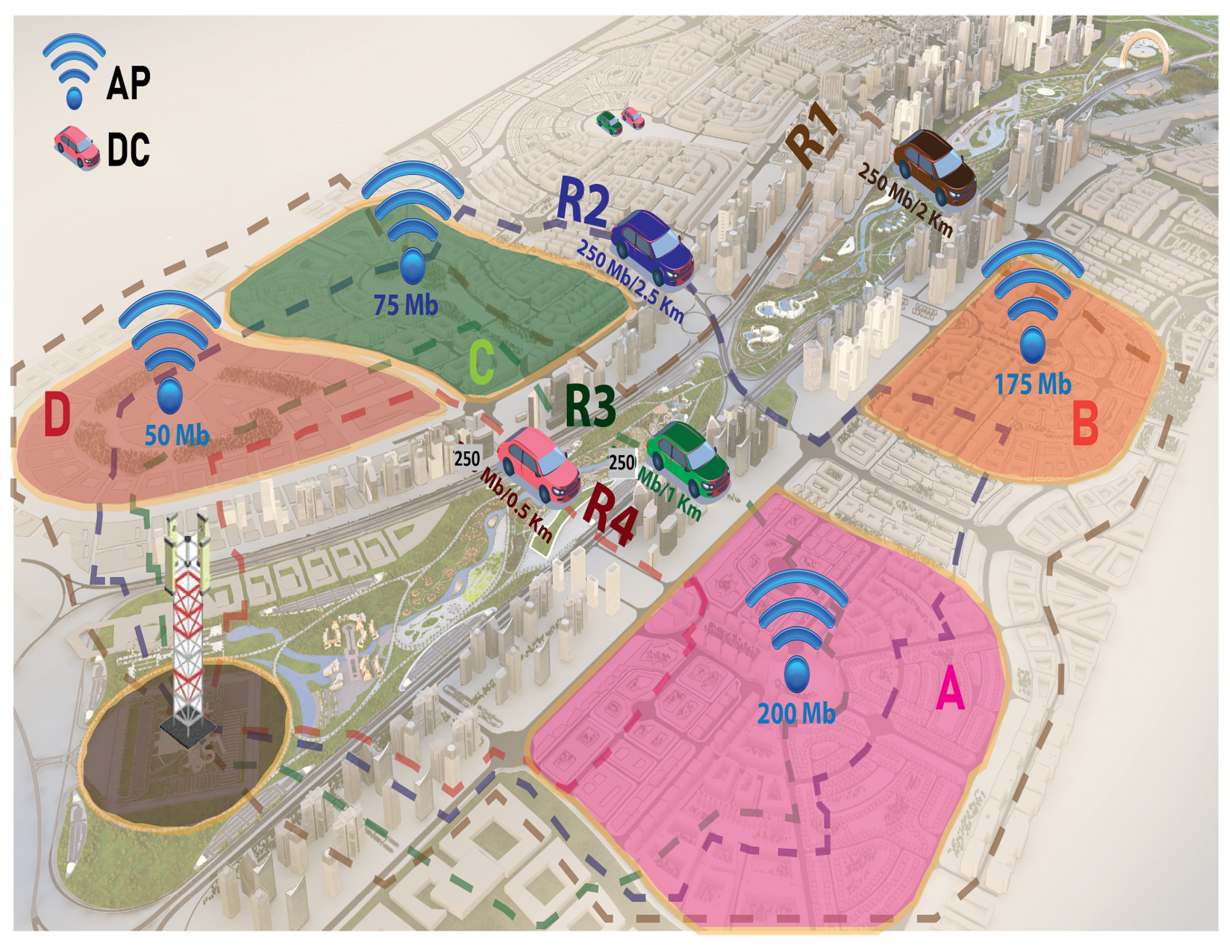
We elaborate more on our proposed BDPP approach in this section, through a traditional delay-tolerant communication scenario in an urban area. We present an example of the APs in four regions A, B, C, and D of a city, with one or more routes connecting to the BS via some D-collectors, as shown in Figure 6.

Consider that each D-collector route has its travel distance and end-to-end storage capability as suggested in the format (capacity/distance constraints) of the BDPP approach, which is also shown in Figure 6. These features are according to the routing table exchange between D-collectors and APs. By using our fitness function in Equation (12), the BDPP will select a minimum D-collector without violating the D-collector capacity constraints and minimum distance travel criteria.

For example, AP B in Figure 6 wants to deliver packets with a data load that necessitates a D-collector capability of at least 175 MB. BDPP found three different routes R1, R2, and R3 connecting Access Point B to the BS. All these three routes satisfy the capacity constraints. Hence, the least distance route among these three will be selected, and it is route R3. It is also possible to serve AP C, as the D-collector still satisfies the capacity constraint. The D-collector route R4, which passes through cities A and D, will then be used to transmit its corresponding data. Therefore, the routes chosen will be:

Route 1: BS B C

Route 2: BS A D

If we choose R1 or R2 instead of R3, the D-collector capacity constraint is met, but it does not provide the total minimum distance travel criteria. Selecting the least count of D-collectors in the vicinity of each AP is attained through frequent exchange of logging records and routing tables with Base Stations, to transmit delay tolerant data packets in the network [18]. At the start of each triggered round, this selection method is repeated.

6. Simulation Results and Performance Evaluation

This section is divided into three parts. In the first part, we elaborate on the simulation setup and parameters used. The second part of this section evaluates the proposed BDPP approach’s correctness using a preliminary study based on practical route instance experiments. Then, in the third part, we compare BDPP with HS [57], EF [56], HCPF [18] and LoRaWAN [58] (smart grid meters data delivery in IoT environment) with reference to various design aspects that influence the overall cost in a medium-sized city. Using MATLAB R2020a, we simulated heterogeneous networks generated randomly that represent the PS environment in a smart city. We assessed the performance of BDPP by running our demo 10 times for each test and averaging the results.

6.1. Simulation Setup and Parameters Used

The whole network area of the smart city was divided into a set of APs and a BS. We assumed a total of up to 100 APs, and between these APs, a number of D-collectors, a subset of mobile public transportation vehicles, were driven. In this work, we analyze our IPDCA in terms of the following metrics:

• AP Count: It is the cumulative number of APs in the network and reflects the network’s scale. This setting has a direct influence on the overall distance traveled.
• D-collector count: It represents the number of D-collectors being used to visit all devices on the network.
• Total distance travelled: It represents the Euclidean distance of separation between successive APs that the D-collector visits while moving on a route and is measured in $km$. In each solution, this setting has been selected to represent the energy and time consumed.
• Cost: This is the estimated weighted value of the fitness function given in Equation (12).
• Throughput: It defines the total data arrived in unit time (second) to the BS via D-collectors and it is measured in Mbps (It also indicates the QoS (quality of service) in the system).
• Area size: This metric reflects the area of the target region as measured in $K{m}^2$.
• APs Load: It is the quantity of data that will be sent from the APs to the BS through the D-collector. It represents the data traffic generated in a smart city network, and is measured in Mbytes.
• D-collector Capacity: It is the highest storage ability (in Mbytes) of a D-collector and the sum of the data loads collected by the D-collector will never exceed the capacity of that D-collector.

Different parameters adopted in our study are shown in

Table 1. Network parameters.

Network Parameters	Value
AP Count	100
AP Radius	100 m
Transmission Bandwidth	5 MHZ
D-collector Speed	15–60 Km/hr
Access Point Transmit power	20 mW
Expected Failure rate	0.001/hr

and

Table 2. BDPP parameters.

Parameters	Value
Maximum number of generation	100
Population Size	100
$A_i,r_i,{\beta }_1,rand$	$\in [0.0,1.0]$
ran	$\in [1,2]$
$f_{mn}$	1
$f_{mx}$	Number of APs

. In this research, the parameters of the network components used are mainly driven from [18] and LoRaWAN parameters are taken from [58]. Depending on the node location and density, the network assumed in this work is random. We use the BDPP algorithm in order to pick the most suitable D-collector trajectory on these randomly generated networks. The simulation results of the IPDCA approach are then compared with other existing baseline methods. The same issue raised in this research is addressed by these baseline approaches: Hybrid Search (HS), the Effective Fitness (EF), HCPF, and the LoRaWAN; however, different path planning techniques are used in them.

6.2. Experimental Setup and Results

Several real experimental Vehicular Routing Problem (VRP) instances from [67] are used to validate our proposed BDPP approach in this section. For this, we compare BDPP with pure GA and HCPF (Hybrid GA and improved Local search) algorithms. Genetic-based parameters of GA and HCPF algorithms are taken from [18]. Validation experiments are performed with the related location set, D-collector capacity and the APs demands, for each symmetrical capacitated VRP instance given in [67]. All the used VRP instances are given in

Table 3. VRP instances for BDPP evaluation.

VRP Problem Instance	Known Best Value [67]	M	K	C
A-n34-k5	778	33	5	100
F-n72-k4	238	71	4	3000
F-n45-k4	724	44	4	2010
E-n101-k8	815	100	7	200
E-n51-k5	521	50	5	160
E-n30-k3	534	29	3	4500
E-n23-k3	569	22	3	4500
E-n22-k4	375	21	4	6000
B-n39-k5	549	38	5	100
A-n80-k10	1763	79	10	100

. Where M indicates the APs number, K is the optimal number of D-collectors required and C is the D-collector capacity. As provided in Table 3, the optimal number of D-collectors with minimum total distance is achieved with total convergence in each run of the experiment. The standard deviation and average error values are both zero, indicating that the proposed solution is stable.

From Figure 7, Figure 8 and Figure 9, we can observe the change in total distance with varying AP load traffic. For this experiment we set the D- Collector capacity fixed and AP load varies from 1 to 6. From these figures, it is clear that while increasing the AP load, the total distance is also increasing. From Figure 7 we can observe that the convergence is not sufficient in GA because it is only applying global search in GA. In Figure 8 and Figure 9, HCPF and BDPP achieve convergence very easily after a number of iteration, this is because of the combined effect of global and local search in both algorithms. BDPP provides a better result than HCPF, due to the use of a multitude of local search methods along with global search.

Figure 10, Figure 11 and Figure 12 depict the effect of D-collector capacity with total distance. For these experiments, we have set AP load as 1 for all instances and D-collector capacity varies from 10 to 60. It is clear from these figures that when the D-collector capacity increases, the total distance is decreasing. From Figure 10, for GA the convergence is not sufficient without using the local search method. In Figure 11 and Figure 12 HCPF and BDPP are converging better than GA. Comparing the three results BDPP provides a better result than HCPF and GA. GA provides the worst result than HCPF and BDPP.

Figure 13 provides the effect of AP count with total distance. For this experiment, we used the E-n101-k8 VRP instance (given in Table 3). This contains a total of 100 APs, and we selected AP locations randomly from this set (10, 20, 30, 40, 50, 60, 70, 80, 90). From this figure we can observe that as the AP count increases, total distance also increases; and it is also clear that BDPP works better than HCPF and GA.

6.3. Simulation Results

Simulation results for different data load combinations and D-collector capacities under: EF, HS, LoRaWAN, HCPF, and two versions of BDPP are shown in this section. The BDPP versions vary on the basis of their stopping criteria, which is the maximum number of generations. The maximum generation for BDPP-1 is 200 and the maximum generation for BDPP-2 is 100. The simulation is done for randomly generated locations and then repeated 10 times on the same set. The average results are shown in Figure 14, Figure 15, Figure 16, Figure 17 and Figure 18.

In Figure 14, as the AP count increases, we find that all methods, with the exception of the EF-based method, converge to the same overall path distance traveled (about 1900). When the total number of D-collectors used and the traffic load are fixed, it is clear that the overall path distance traveled will hit a limit that cannot be exceeded. In contrast to LoRaWAN, EF, HCPF and HS, BDPP-1 and BDPP-2 are increasing in a consistent manner with respect to the overall distance of the route as the D-collector count increases. This is because of the systematic approach in the proposed BDPP method to optimize the search performance. It is clear that the BDPP-1 is the fastest solution in terms of convergence and still has the least overall path distance traveled. BDPP-2 and HCPF have similar performance when the number of APs ≥30. While the number of APs ≥30, in terms of the overall distance traveled, all approaches will no longer change.

From Figure 15, the impact of data traffic load at APs on the overall path distances of the occupied D-collectors is being examined. Here we used fixed D-collector capacity. In this figure, for all approaches, except for the BDPP-1, the total traveled distance grows while the AP load changes from 10 to 80 MB. For the proposed BDPP method, this shows a great benefit when using a greater value of max generation. BDPP chooses the optimal D-collectors required and thereby it reduces the total distance traveled when it uses fixed D-collector capacity. It is also evident that the graph of HS and EF are increasing monotonically, indicating that the HS and EF are highly sensitive to the AP loads to be transmitted. It is clear that as the AP load rises, BDPP-1 has the least overall traveled distances. We also note that when the AP load ≥70 Mb, the BDPP-2, HCPF and LoRaWAN are no longer able to improve in terms of the overall traveled distances.

The effect of the total distance traveled against the varying capacity of the D-collector is shown in Figure 16. The total distance traveled is decreased when the capacity of the D-collector increases. From this figure, it is evident that HCPF, BDPP-1 and BDPP-2 have almost identical performance when D-collector capacity is ≥60. BDPP-1 shows better performance in terms of total distance traveled. This is because when D-collector capacity increases, our multi-objective fitness function will help to select a path that has the least distance and minimal number of D-collectors and thereby we get better-traveled distance performance. However, as the D-collector capacity increases, HS and EF exhibit the worst performance with respect to the overall traveled distance, and LoRaWAN has a better result than EF and HS, but not as BDPP.

In Figure 17, for all approaches, the D-collector count increases monotonically, while the deployment area size increases. When the area size is ≥3000 km², HS and EF methods show the same performance, and these methods need the highest D-collector count with an increase in the area size. As the area size increases, BDPP-1 needs the lowest D-collector count, which is because the BDPP algorithm takes the optimal number of D-collectors required.

From Figure 18, we can analyze the effect of cost on the average system throughput. For all strategies, the total average system throughput increases, while increasing the cost parameter. However, regarding the total throughput attained, they saturate after achieving a fixed cost value. BDPP-2, HCPF and LoRaWAN have the same performance once the cost of the system reaches a particular value (almost 1000). HS and EF show nearly equal performance for overall cost and have the lowest throughput. BDPP-1, however, outperforms all other methods under all the examined cost values.

In summary, we have compared BDPP with HS, EF, HCPF and LoRaWAN using different design aspects that influence the overall cost in a medium-sized city and from the above results, we observed that the proposed approach is superior to other approaches with respect to both quality and time complexity. It should be observed that the proposed method outperforms other approaches under different parameters’ values and configurations. At the same time, it should also be noted that the chosen parameters and system configurations greatly influence the quality of the solutions and the achieved convergence. It is clear that our IPDCA is less sensitive to the AP load and uses the least number of D-collectors when the area size is increasing. It should be also noted that BDPP with maximum generation gives better results than BDPP with lesser generations.

7. Conclusions

In this work, we have introduced the IPDCA: Intelligent Proficient Data Collection Approach for IoT-Enabled Wireless Sensor Networks in Smart Environments. Our approach is designed based on a two-tier architecture and is capable of handling heterogeneous data sources with mobile D-collectors in urban areas. In this framework, APs will receive the readings of the sensors and initiate requests for data delivery. To deliver the data in a cost-effective manner, we proposed BAT algorithm-based D-collector path planning called BDPP. IPDCA uses a multi-objective fitness function at the top-tier to select the D-collectors path in a smart city environment. This fitness function helps to maximize network gain in terms of the limited number of D-collectors, storage capacity and total distance traveled. The extensive simulation results show that our approach outperforms other approaches with similar objectives in terms of varying parameters such as storage capacity, network size, D-collector count and total distance traveled. Our IPDCA simulation results are provided in two versions with a varying number of generations in BDPP. It is clear that BDPP with maximum generation gives better results than the lesser generations. In BDPP we employed a multitude of local search methods to get the better result in the neighborhood. We succeeded in this and obtained better results when compared to the other methods with similar objectives.

References

1. Hamzei, M.; Jafari Navimipour, N. Toward Efficient Service Composition Techniques in the Internet of Things. IEEE Internet Things J. 2018, 5, 3774–3787. [Google Scholar] [CrossRef]
2. Firouzi, F.; Farahani, B.; Weinberger, M.; DePace, G.; Aliee, F.S. Iot fundamentals: Definitions, architectures, challenges, and promises. Intell. Internet Things 2020, 1, 3–50. [Google Scholar] [CrossRef]
3. Atzori, L.; Morabito, G.; Lera, A. Understanding the internet of things: Definition. Ad Hoc Netw. 2017, 56, 122–140. [Google Scholar] [CrossRef]
4. Omar, D.M.; Khedr, A.M. ERPLBC: Energy Efficient Routing Protocol for Load Balanced Clustering in Wireless Sensor Networks. Ad Hoc Sens. Wirel. Netw. 2018, 42, 145–169. [Google Scholar]
5. Hanif, S.; Khedr, A.M.; Al Aghbari, Z.; Agrawal, D.P. Opportunistically Exploiting Internet of Things for Wireless Sensor Network Routing in Smart Cities. J. Sens. Actuator Netw. 2018, 7, 46. [Google Scholar] [CrossRef] [Green Version]
6. Schoenherr, T. Environmental sustainability initiatives: A comparative analysis of plant efficiencies in Europe and the U.S. IEEE Trans. Eng. Manag. 2013, 60, 353–365. [Google Scholar] [CrossRef]
7. Viitanen, J.; Kingston, R. Smart cities and green growth: Outsourcing democratic and environmental resilience to the global technology sector. Environ. Plan. A 2013, 45. [Google Scholar] [CrossRef] [Green Version]
8. Park, S. D-PARK: User-Centric Smart Parking System over BLE-Beacon Based Internet of Things. Electronics 2021, 10, 541. [Google Scholar] [CrossRef]
9. Su, K.; Li, J.; Fu, H. Smart city and the applications. In Proceedings of the International Conference on Electronics, Communications and Control (ICECC), Ningbo, China, 9–11 September 2011; pp. 1028–1031. [Google Scholar] [CrossRef]
10. Dryjanski, M.; Buczkowski, M.; Ould-Cheikh-Mouhamedou, Y.; Kliks, A. Adoption of Smart Cities with a Practical Smart Building Implementation. IEEE Internet Things Mag. 2020, 3, 58–63. [Google Scholar] [CrossRef]
11. Dutta Pramanik, P.K.; Upadhyaya, B.K.; Pal, S.; Pal, T. Chapter 1-Internet of things, smart sensors, and pervasive systems: Enabling connected and pervasive healthcare. In Advances in Ubiquitous Sensing Applications for Healthcare, Healthcare Data Analytics and Management; Dey, N., Ashour, A.S., Bhatt, C., Fong, S.J., Eds.; Academic Press: Cambridge, MA, USA, 2019; pp. 1–58. ISBN 9780128153680. [Google Scholar]
12. Huang, H.; Savkin, A.V. Optimal path planning for a vehicle collecting data in a Wireless Sensor Network. In Proceedings of the 2016 35th Chinese Control Conference (CCC), Chengdu, China, 27–29 July 2016. [Google Scholar] [CrossRef]
13. Nha, V.T.N.; Djahel, S.; Murphy, J. A comparative study of vehicles’ routing algorithms for route planning in smart cities. In Proceedings of the First International Workshop on Vehicular Traffic Management for Smart Cities (VTM), Dublin, Ireland, 20 November 2012; pp. 1–6. [Google Scholar]
14. Raj, R.; Babu, S.; Benson, K.; Jain, G.; Manoj, B.S.; Venkatasubramanian, N. Efficient Path Rescheduling of Heterogeneous Mobile Data Collectors for Dynamic Events in Shanty Town Emergency Response. In Proceedings of the 2015 IEEE Global Communications Conference (GLOBECOM), San Diego, CA, USA, 6–10 December 2015. [Google Scholar] [CrossRef]
15. Ma, X.; Kacimi, R.; Dhaou, R. Fairness-aware UAV-assisted data collection in mobile wireless sensor networks. In Proceedings of the 2016 International Wireless Communications and Mobile Computing Conference (IWCMC), Paphos, Cyprus, 5–9 September 2016. [Google Scholar] [CrossRef] [Green Version]
16. Onishi, H.; Asaka, T. Efficient data collection for participatory sensing using smartphones. In Proceedings of the 2016 18th Asia-Pacific Network Operations and Management Symposium (APNOMS), Kanazawa, Japan, 5–7 October 2016. [Google Scholar] [CrossRef]
17. Muhammad, A.S.; Soliman, S.S.; Badawi, A. On the mobility of data collectors in WSN. In Proceedings of the 2017 12th International Conference on Computer Engineering and Systems (ICCES), Cairo, Egypt, 19–20 December 2017. [Google Scholar] [CrossRef]
18. Al-Turjman, F. Mobile Couriers’ selection for the Smart-grid in Smart-cities’ Pervasive Sensing. Future Gener. Comput. Syst. 2018, 82, 327–341. [Google Scholar] [CrossRef]
19. Biglarbegian, M.; Al-Turjman, F. Path planning for data collectors in Precision Agriculture WSNs. In Proceedings of the 2014 International Wireless Communications and Mobile Computing Conference (IWCMC), Nicosia, Cyprus, 4–8 August 2014; pp. 483–487. [Google Scholar] [CrossRef]
20. Aziz, A.; Singh, K.; Osamy, W.; Khedr, A.M. Effective Algorithm for Optimizing Compressive Sensing in IoT and Periodic Monitoring Applications. J. Netw. Comput. Appl. 2019, 126, 12–28. [Google Scholar] [CrossRef]
21. Osamy, W.; Salim, A.; Khedr, A.M. An Information Entropy Based-Clustering Algorithm in Heterogeneous Wireless Sensor Networks. Wirel. Netw. 2020, 26, 1869–1886. [Google Scholar] [CrossRef]
22. Salim, A.; Osamy, W.; Khedr, A.M. IBLEACH: Effective LEACH Protocol for Wireless Sensor Networks. Wirel. Netw. 2014, 20, 1515–1525. [Google Scholar] [CrossRef]
23. Khedr, A.M.; Aziz, A.; Osamy, W. Successors of PEGASIS protocol: A comprehensive survey. Comput. Sci. Rev. 2021, 39, 100368. [Google Scholar] [CrossRef]
24. Osamy, W.; El-Sawy, A.A.; Khedr, A.M. Effective TDMA Scheduling for Data Collection in Tree Based Wireless Sensor Networks. Peer-to-Peer Netw. Appl. 2020, 13, 796–815. [Google Scholar] [CrossRef]
25. Osamy, W.; Khedr, A.M.; Aziz, A.; El-Sawy, A. Cluster-Tree Routing Scheme for Data Gathering in Periodic Monitoring Applications. IEEE Access 2019, 6, 77372–77387. [Google Scholar] [CrossRef]
26. Hashim Raza Bukhari, S.; Siraj, S.; Husain Rehmani, M. Wireless sensor networks in smart cities: Applications of channel bonding to meet data communication requirements. Transp. Power Grid Smart Cities Commun. Netw. Serv. 2018, 247–268. [Google Scholar] [CrossRef]
27. Cetinkaya, O.; Akan, O.B. Use of wireless sensor networks in smart homes. In Emerging Communication Technologies Based on Wireless Sensor Networks: Current Research and Future Applications; CRC Press: Boca Raton, FL, USA, 2016; pp. 233–258. [Google Scholar]
28. Morello, R.; Mukhopadhyay, S.C.; Liu, Z.; Slomovitz, D.; Samantaray, S.R. Advances on sensing technologies for smart cities and power grids: A review. IEEE Sens. J. 2017, 17, 7596–7610. [Google Scholar] [CrossRef]
29. Ghaleb, M.; Subramaniam, S.; Othman, M.; Zukarnain, Z. Predetermined path of mobile data gathering in wireless sensor networks based on network layout. EURASIP J. Wirel. Commun. Netw. 2014, 2014, 1–18. [Google Scholar] [CrossRef] [Green Version]
30. Mohan, B.A.; Sarojadevi, H. A hybrid approach for data collection using multiple mobile nodes in WSN (HADMMN). In Proceedings of the 2016 IEEE International Conference on Recent Trends in Electronics, Information and Communication Technology (RTEICT), Bangalore, India, 20–21 May 2016; pp. 711–714. [Google Scholar] [CrossRef]
31. Mohan, B.A.; Sarojadevi, H. Energy-Efficient Hybrid Protocol for Routing Based on Mobile Data Collectors in Wireless Sensor Network. In Smart Computing and Informatics. Smart Innovation, Systems and Technologies; Satapathy, S., Bhateja, V., Das, S., Eds.; Springer: Singapore, 2018; Volume 77. [Google Scholar] [CrossRef]
32. Singh, S.K.; Kumar, P. A comprehensive survey on trajectory schemes for data collection using mobile elements in WSNs. J. Ambient Intell. Humaniz. Comput. 2020, 11, 291–312. [Google Scholar] [CrossRef]
33. Kumar, N.; Dash, D. Flow based efficient data gathering in wireless sensor network using path-constrained mobile sink. J. Ambient Intell. Humaniz. Comput. 2020, 11, 1163–1175. [Google Scholar] [CrossRef]
34. Raj Pravija, P.V.; Khedr, A.M.; Al Aghbari, Z. Data gathering via mobile sink in WSNs using game theory and enhanced ant colony optimization. Wirel. Netw. 2020, 26, 2983–2998. [Google Scholar]
35. Prabaharan, G.; Jayashri, S. An optimal mobile data gathering in small scale WSN by power saving adaptive clustering techniques. J. Ambient Intell. Humaniz. Comput. 2020, 12, 3989–3997. [Google Scholar] [CrossRef]
36. Fellah, K.; Kechar, B. New approach based on Hilbert curve for energy efficient data collection in WSN with mobile sink. IET Wirel. Sens. Syst. 2020, 10, 214–220. [Google Scholar] [CrossRef]
37. Verma, A.; Kumar, S.; Gautam, P.; Rashid, T.; Kumar, A. Fuzzy logic based effective clustering of homogeneous wireless sensor networks for mobile sink. IEEE Sens. J. 2020, 20, 5615–5623. [Google Scholar] [CrossRef]
38. Şenturk, I. A Steiner Zone Approach for Mobile Data Collection in Partitioned Wireless Sensor Networks. Bilişim Teknol. Derg. 2020, 13, 217–224. [Google Scholar] [CrossRef]
39. Kamarei, M.; Patooghy, A.; Shahsavari, Z.; Salehi, M.J. Lifetime expansion in WSNs using mobile data collector: A learning automata approach. J. King Saud Univ. Comput. Inf. Sci. 2020, 32, 65–72. [Google Scholar] [CrossRef]
40. Chukwuemeka, C.; Chimsom, I.; Habib, M.K. Integrated Development of Collaborative Mobile Robots and WSNs Supported by Cloud Service. In Proceedings of the 2020 6th International Conference on Mechatronics and Robotics Engineering (ICMRE), Barcelona, Spain, 12–15 February 2020; pp. 26–31. [Google Scholar]
41. Meddah, M.; Haddad, R.; Ezzedine, T. Fuzzy Tree Clustering Algorithm with Mobile Data Collectors in Wireless Sensor Networks. Wirel. Pers. Commun. 2020, 115, 2645–2665. [Google Scholar] [CrossRef]
42. Wu, Q.; Sun, P.; Boukerche, A. A Novel Data Collector Path Optimization Method for Lifetime Prolonging in Wireless Sensor Networks. In Proceedings of the 2019 IEEE Global Communications Conference (GLOBECOM), Waikoloa, HI, USA, 9–13 December 2019; pp. 1–6. [Google Scholar] [CrossRef]
43. Konstantopoulos, C.; Vathis, N.; Pantziou, G.; Gavalas, D. Employing Mobile Elements for Delay-Constrained Data Gathering in WSNs. Comput. Netw. 2018, 135, 108–131. [Google Scholar] [CrossRef]
44. Akber, S.M.A.; Khan, I.A.; Muhammad, S.S.; Mohsin, S.M.; Khan, I.A.; Shamshirband, S.; Chronopoulos, A.T. Data volume-based data gathering in wsns using mobile data collector. In Proceedings of the 22nd International Database Engineering and Applications Symposium, Villa San Giovanni, Italy, 18 June 2018; pp. 199–207. [Google Scholar]
45. Cecchinel, C.; Jimenez, M.; Mosser, S.; Riveill, M. An architecture to support the collection of big data in the internet of things. In Proceedings of the 2014 IEEE World Congress on Services, Anchorage, AK, USA, 27 June–2 July 2014; pp. 442–449. [Google Scholar]
46. Rahman, T.; Yao, X.; Tao, G. Consistent data collection and assortment in the progression of continuous objects in iot. IEEE Access 2018, 6, 51875–51885. [Google Scholar] [CrossRef]
47. Xu, G.; Ngai, E.C.-H.; Liu, J. Ubiquitous transmission of multimedia sensor data in internet of things. IEEE Internet Things J. 2017, 5, 403–414. [Google Scholar] [CrossRef]
48. Tang, L.; Guo, H.; Wu, R.; Fan, B. Adaptive Dual-Mode Routing-Based Mobile Data Gathering Algorithm in Rechargeable Wireless Sensor Networks for Internet of Things. Appl. Sci. 2020, 10, 1821. [Google Scholar] [CrossRef] [Green Version]
49. Singh, G.; Al-Turjman, F. A data delivery framework for cognitive information-centric sensor networks in smart outdoor monitoring. Comput. Commun. J. 2016, 74, 38–51. [Google Scholar] [CrossRef]
50. Masoud, A. A harmonic potential field approach for joint planning and control of a rigid, separable nonholonomic, mobile robot. Robot. Auton. Syst. 2013, 61, 593–615. [Google Scholar] [CrossRef] [Green Version]
51. Zhang, Y.; Fattahi, N.; Li, W. Probabilistic roadmap with self-learning for path planning of a mobile robot in a dynamic and unstructured environment. In Proceedings of the IEEE International Conference on Mechatronics and Automation (ICMA), Takamatsu, Japan, 4–7 August 2013. [Google Scholar]
52. Al-Turjman, F.; Hassanein, H.; Ibnkahla, M. Quantifying connectivity in wireless sensor networks with grid-based deployments. J. Netw. Comput. Appl. 2013, 36, 368–377. [Google Scholar] [CrossRef]
53. Connell, D.; Manh La, H. Extended rapidly exploring random tree–based dynamic path planning and replanning for mobile robots. Int. J. Adv. Robot. Syst. 2018, 15, 1729881418773874. [Google Scholar] [CrossRef] [Green Version]
54. Wang, L.; Yang, S.X.; Biglarbegian, M. A fuzzy logic based bio-inspired system for mobile robot navigation. In Proceedings of the IEEE Conference on Multisensor Fusion and Integration for Intelligent Systems (MFI), Hamburg, Germany, 13–15 September 2012. [Google Scholar]
55. Al-Turjman, F.; Hassanein, H.; Ibnkahla, M. Towards prolonged lifetime for deployed WSNs in outdoor environment monitoring. Ad Hoc Netw. J. 2015, 24, 172–185. [Google Scholar] [CrossRef]
56. Shih, C.-C.; Horng, M.-F.; Pan, T.-C.; Pan, J.-C.; Chen, C.-Y. A genetic-based effective approach to path-planning of autonomous underwater glider with upstream-current avoidance in variable oceans. Soft Comput. 2016, 21, 5369–5386. [Google Scholar] [CrossRef]
57. Soulignac, M. Feasible and optimal path planning in strong current fields. IEEE Trans. Robot. 2011. [Google Scholar] [CrossRef]
58. Filho, H.G.S.; Filho, J.P.; Moreli, V. The adequacy of LoRaWAN on smart grids: A comparison with RF mesh technology. In Proceedings of the IEEE Smart Cities Conference, ISC2, Trento, Italy,, 12–15 September 2016. [Google Scholar]
59. Senturk, I.F.; Coulibaly, S. Mobile Data Collection in Smart City Applications: The Impact of Precedence based Route Planning on Data Latency. J. Innov. Sci. Eng. 2020, 4, 22–34. [Google Scholar]
60. Al-Turjman, F.; Karakoc, M.; Gunay, M. Path planning for mobile DCs in future cities. Ann. Telecommun. 2016, 72, 119–129. [Google Scholar] [CrossRef]
61. Alsalih, W.; Hassanein, H.S.; Akl, S. Routing to a Mobile Data Collector on a Predefined Trajectory. In Proceedings of the 2009 IEEE International Conference on Communications, Dresden, Germany, 14–18 June 2009. [Google Scholar] [CrossRef]
62. Vazifehdan, J.; Prasad, R.V.; Jacobsson, M.; Niemegeers, I. An analytical energy consumption model for packet transfer over wireless links. IEEE Commun. Lett. 2011, 16, 30–33. [Google Scholar] [CrossRef]
63. Yang, X.-S. A new metaheuristic bat-inspired algorithm. In Nature Inspired Cooperative Strategies for Optimization (NICSO 2010); Springer: Berlin, Germany, 2010; pp. 65–74. [Google Scholar]
64. Yang, X.-S.; Gandomi, A.H. Bat algorithm: A novel approach for global engineering optimization. Eng. Comput. 2012, 29, 464–483. [Google Scholar] [CrossRef] [Green Version]
65. Saji, Y.; Essaid Riffi, M. A novel discrete bat algorithm for solving the travelling salesman problem. Neural Comput. Appl. 2016, 27, 1853–1866. [Google Scholar] [CrossRef]
66. Cai, Y.; Qi, Y.; Cai, H.; Huang, H.; Chen, H. Chaotic discrete bat algorithm for capacitated vehicle routing problem. Int. J. Auton. Adapt. Commun. Syst. 2019, 12, 91. [Google Scholar] [CrossRef]
67. Networking and Emerging Optimization, Capacitated VRP Instances—Vehicle Routing Problem. 2016. Available online: http://neo.lcc.uma.es/vrp/vrpinstances/capacitated-vrp-instances/ (accessed on 1 April 2021).
Figure 1. Two-layer architecture.
Electronics 10 00997 g001
Figure 2. Data gathering in smart city through D-collectors.
Electronics 10 00997 g002
Figure 3. Flow diagram of BDPP.
Electronics 10 00997 g003
Figure 4. Two-exchange crossover algorithm for D-collector path planning.
Electronics 10 00997 g004
Figure 5. Local search methods.
Electronics 10 00997 g005
Figure 6. Example scenario.
Electronics 10 00997 g006
Figure 7. AP load vs. total distance (GA).
Electronics 10 00997 g007
Figure 8. AP load vs. total distance (HCPF).
Electronics 10 00997 g008
Figure 9. AP load vs. total distance (BDPP).
Electronics 10 00997 g009
Figure 10. D-collector capacity vs. total distance (GA).
Electronics 10 00997 g010
Figure 11. D-collector capacity vs. total distance (HCPF).
Electronics 10 00997 g011
Figure 12. D-collector capacity vs. total distance (BDPP).
Electronics 10 00997 g012
Figure 13. AP count vs. total distance.
Electronics 10 00997 g013
Figure 14. AP count vs. total distance.
Electronics 10 00997 g014
Figure 15. AP load vs. total distance.
Electronics 10 00997 g015
Figure 16. D-collector capacity vs. total distance.
Electronics 10 00997 g016
Figure 17. Area size vs. D-collector count.
Electronics 10 00997 g017
Figure 18. Total cost vs. throughput.
Electronics 10 00997 g018