Planar-Equirectangular Image Stitching

Abstract

The 360° cameras have served as a convenient tool for people to record their special moments or everyday lives. The supported panoramic view allowed for an immersive experience with a virtual reality (VR) headset, thus adding viewer enjoyment. Nevertheless, they cannot deliver the best angular resolution images that a perspective camera may support. We put forward a solution by placing the perspective camera planar image onto the pertinent 360° camera equirectangular image region of interest (ROI) through planar-equirectangular image stitching. The proposed method includes (1) tangent image-based stitching pipeline to solve the equirectangular image spherical distortion, (2) feature matching scheme to increase correct feature match count, (3) ROI detection to find the relevant ROI on the equirectangular image, and (4) human visual system (HVS)-based image alignment to tackle the parallax error. The qualitative and quantitative experiments showed improvement of the proposed planar-equirectangular image stitching over existing approaches on a collected dataset: (1) less distortion on the stitching result, (2) 29.0% increased on correct matches, (3) 5.72° ROI position error from the ground truth and (4) lower aggregated alignment-distortion error over existing alignment approaches. We discuss possible improvement points and future research directions.

1. Introduction

The proliferation of inexpensive 360° cameras has instigated various use of the camera, not only for research [1,2], but also for daily life [3,4,5]. Consumers have been using the 360° cameras for recording and possibly sharing their social activities such as trips, holidays, or parties with others [3]. Some of them will even use a virtual reality (VR) headset to view the captured scene with great immersion, allowing them to re-experience the moments [6]. While mindlessly looking around the captured scene, they can find new things or unanticipated events, make them want to see the details of what was happening. Nevertheless, the view from 360° camera is not suitable for the detailed view because it cannot provide a high angular resolution view as much as perspective cameras could offer [7]. It would be interesting to search online for the perspective camera planar images that captured similar scenes then stitch them on top of the relevant region of interest (ROI). We bring forward an image-stitching algorithm that supports the high-resolution view on the ROI. The algorithm aims to stitch the high angular resolution planar image (HPI) onto the 360° equirectangular image (EI).

The image stitching process is generally used to combine multiple overlapping input images into a single wide field of view (FOV) output image [8], i.e., planar-planar image stitching. When stitching the input images, it is crucial to establish a well-aligned overlapping region to create a smooth view in the stitched output image. Researchers proposed several image transformation models to align the adjacent input images [9].

Nonetheless, the transformation models cannot be directly applied to our case where we stitch an HPI on a 360° EI. First, their models are designed for stitching two planar images rather than stitching a planar image on an equirectangular one. The equirectangular type image possesses stronger spherical image distortion than the planar one [10]. Second, their stitching algorithms were designed for stitching side-by-side images. The alignment constraint only applies for one side (i.e., the overlapping one) of each input image, allowing the other side free. In cases of multiple input images, the transformation model of every input image can also be altered. On the contrary, our goal is to put the HPI on top of their corresponding EI ROI. The EI acts as a template that the form should be fixed, leaving the HPI as the only input to be modified. As the EI also covers the whole HPI region, these situations can lead to alignment-distortion error trade-off (see Section 4.3) when parallax error occurred.

We propose a tangent image (TI)-based approach to mitigate the strong spherical image distortion. TIs are generated by projecting the EI onto the icosahedron faces. The projection produces planar images with predetermined sizes. We perform image stitching steps, such as feature extraction-matching and image alignment, on the TI before reprojecting the stitching result back to the equirectangular coordinate.

We design an image alignment algorithm inspired by the human visual system (HVS) to solve the alignment-distortion trade-off. HVS has a much greater resolution in the central visual field compared to the boundary [11]. Humans used the center vision (i.e., foveal vision) to resolve the focused object’s detail resolution. On the other hand, the boundary vision (i.e., peripheral vision) exists mainly to provide low-resolution cues to guide the fovea movements. Likewise, the proposed algorithm intends to keep the central region less distorted while minimizing the boundary region’s misalignment.

One critical step to perform the planar-equirectangular image stitching is to locate the suitable ROI locations on the EI. Supposing we have a collection of HPIs that depict various spots in one EI, how could we best detect the ROI positions each HPI portrays? ROI detection is a crucial step to determine the TI used for the follow-up alignment step. We consequently put forward an ROI detection algorithm that uses base-level icosahedron: generating the base-level TIs. The detection algorithm identifies an ROI tangent image (ROI-TI): the TI that resembles the targeted HPI through a coarse-to-fine searching process. The ROI-TI position is refined incrementally afterward.

Both image alignment and ROI detection step quality rely upon the excellence of feature matching. We devise an enhanced version of existing grid motion statistics (GMS) that uses brute-force (BF) matcher [12]. We use k-Nearest Neighbor (kNN) matcher to increase the number of correct feature matches, indirectly increasing the matched features distribution. The underlining idea is that, instead of rejecting the false matches after the GMS process, we repeat the GMS process after changing the previously rejected TIs features corresponding pairs: from the current closest to the next closest correspondence.

To summarize, our main contribution is introducing a new image stitching algorithm for placing an HPI on the corresponding EI ROI, and it includes:

C1. 

TI-based planar-equirectangular stitching pipeline.

C2. 

HPI-EI ROI detection algorithm.

C3. 

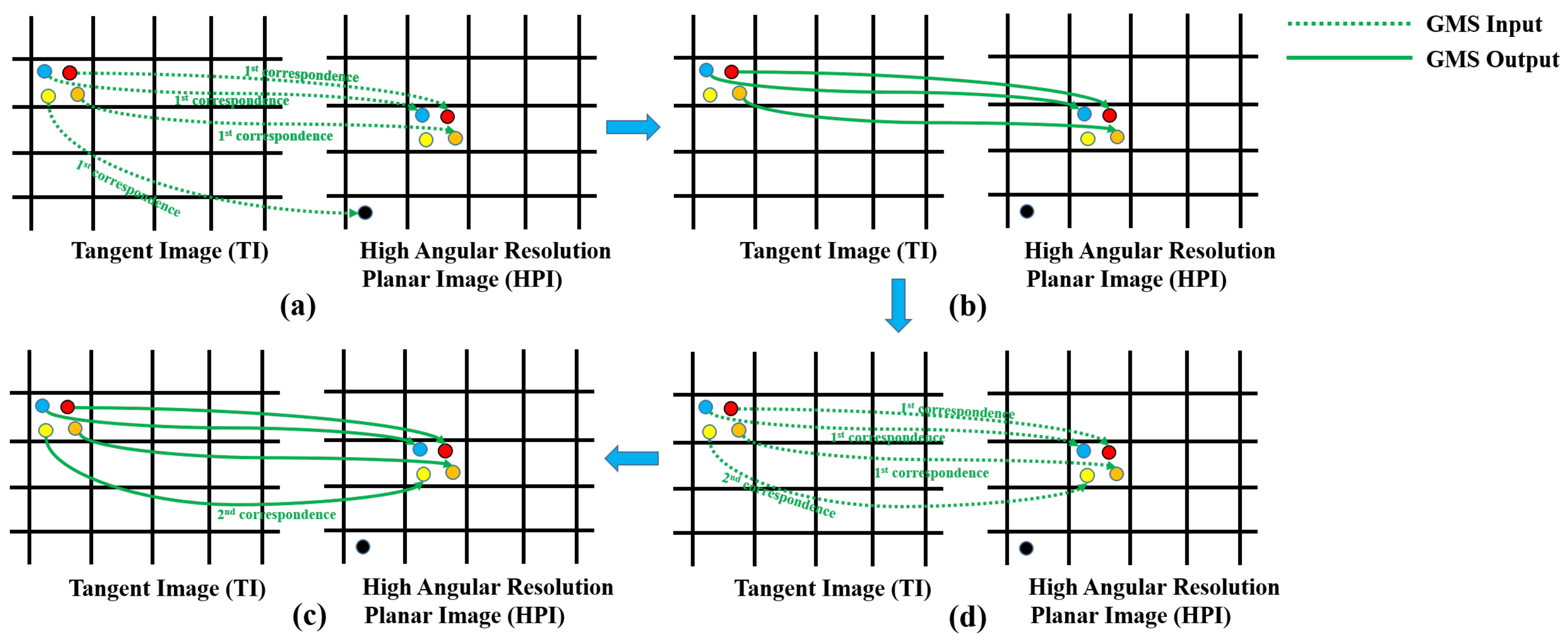
kNN-based GMS feature matching algorithm.

C4. 

HVS-based image alignment algorithm.

We introduced the background case to perform the planar-equirectangular image stitching in this section. We next explain the past and current works on the image stitching in Section 2; emphasizing the problems found in existing approaches for the planar-equirectangular case. We propose the TI-based image stitching solution to solve the problems; explain the TI underlying theory in Section 3 and the proposed stitching in Section 4. We performed the related experiments and discussed the results in Section 5. We present the conclusion and point out the future research directions in Section 6.

2. Related Works

2.1. Planar-Planar Image Stitching

Planar-planar image stitching algorithms aim to join multiple overlapping planar images into a wider FOV or panoramic image [9]. The algorithm is principally designed to tackle artifacts on the overlapping region while keeping the stitching result natural [13], i.e., less distorted. One of the key factors influencing the artifacts’ level is the quality of the image alignment step. Well-aligned input images are desirable to impose a lower requirement on the subsequent deghosting and postprocessing [14].

Image alignment is an act to transform the input images, making the adjacent ones aligned. The process focused on finding the geometric relationships (i.e., geometry models) within each input. Researchers have recently strived to find the geometry models based on sparse feature matching [9]. The goal is to attain the models that best minimize the feature pairs alignment error.

Existing feature matching-based image alignment methods can be grouped into global and local hybrid transformation [9]. The global methods transform the image by applying the same geometry model on a group of pixels. The simplest version used a single model, such as projective [15,16] or affine, for the entire image region. Due to its simplicity, the model only performs well if the inputs differ purely rotational or contain only one plane. The one plane characteristic mostly valid only for scenes captured far away from the camera. To solve more complicated situations where the captured scene consisted of different planes, Gao et al. [17] suggested the dual-homography method. They divided the image into two dominant planes (i.e., ground and distant), with each plane have its geometry model. Regardless, these methods demand the scene to have a certain number of dominant planes.

The methods belong to the local hybrid transformation model treat image as a mesh. The image mesh is divided into grids of vertices; each corresponds to a different transformation model. One well-known method that belongs to this category is the as-projective-as-possible (APAP) approach [14]. They attributed each vertex to a separate homography model. They estimated the model by assigning various weight values for each feature pairs depending on their location relative to the vertex. This separated model designation allows each vertex to align themselves independently to minimize the closest feature pair alignment error. Although the model independence allowed them to receive excellent performance on aligning the input images, it also prompted a distortion problem. For instance, the stitching result will not be likely able to preserve rigid or straight objects [9]. Researchers [18,19] have been adding additional constraints, such as similarity [20], to reduce the distortion. However, the constraints inclusion costs higher computational time.

2.2. Non-Planar Image Stitching

Compared to planar-planar image stitching, there are only a few researchers who attempted to stitch non-planar images. Dornaika et al. [21] tried to create a multi-resolution image from a pair of wide-angle low-resolution and high-resolution image for surveillance application. Instead of employing sparse feature matching, they used pixel-based correspondences and homography models to perform image alignment. While they had a similar purpose, we plan to perform the stitching on the EI whose higher image distortion than their wide-angle image.

Dong et al. [22] stitched wide-angle images on a fisheye-lens video. As they implemented a planar feature extractor, the matching accuracy was initially low. They devised a multi-homography inlier selection method to improve the accuracy. They estimated a global homography and multiple local homographies from the correct matches. They finally constructed the stitching result by combining the weighted global and local homographies. The research showed that modifications of existing planar image processing were essential to handle image distortion on non-planar image stitching.

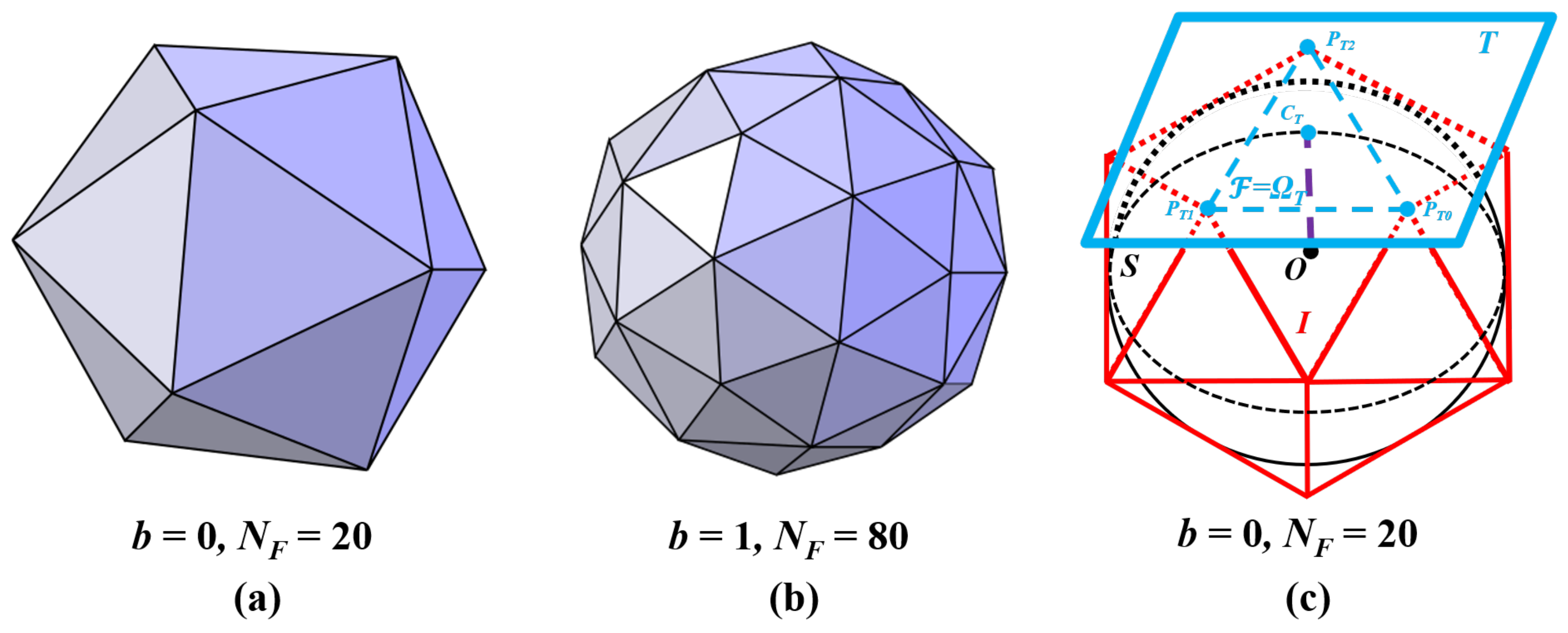
2.3. Icosahedron to Reduce Equirectangular Image (EI) Distortion

High spherical image distortion on the EI makes the existing image processing algorithm designed for planar image perform poorly. Recent approaches attempted to solve the issue by adopting icosahedral sphere representation, i.e., icosahedron. At the base level, the icosahedron consists of 12 vertices and 20 faces. The subdivision along the vertices and faces will cause the icosahedron to resemble a sphere closer. The higher subdivision, smaller spherical distortion will be [23]. The distance between vertices and faces will be similar to each other.

Zhao et al. [24] introduced a spherical-based feature extractor, spherical oriented FAST and Rotated BRIEF (SPHORB): the spherical version of the planar ORB [25]. The SPHORB detects and describes the features directly on the geodesic grid formed from the icosahedron subdivision. They demonstrated planar-equirectangular feature matching, showing higher accuracy of the SPHORB compared to the ORB. Unfortunately, the test was conducted only on two image sets and on the less-distorted equirectangular ROI.

Eder et al. [10] formulized TIs creation through gnomonic projection [26] on the icosahedron face. They introduced a visibility region on the TIs to assess the spherical image distortion. The higher the icosahedron level, the smaller the distortion on the visibility region will be, thus allowing existing planar image processing to work better. They used the visibility region to mask acceptable features on each TI for simple equirectangular feature extraction demonstration.

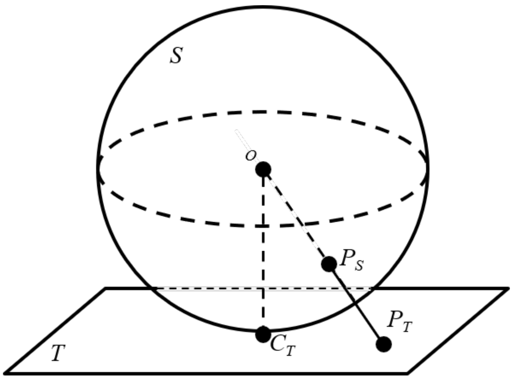
3. Tangent Images (TIs)

In this section, we would like to explain some theories underlying our TI-based planar-equirectangular image stitching. We first explain how to generate the TI from the EI. We also describe how to map from one TI back to the EI or the other TI. At last, we would like to explain the procedure of TI-based feature extraction-matching.

3.1. Tangent Images (TIs) Creation

We intend to generate a TI T from an EI E. In other words, we seek to map the EI pixels $P_E\in E$ onto the TI $P_T\in T$. First, we map the pixel $P_E$ to a unit sphere $P_S\in S$:

$$\begin{array}{cc}\hfill {\lambda }_S& ={\displaystyle \frac{2\pi x_E}{W_E}}\hfill \\ \hfill {\varphi }_S& ={\displaystyle \frac{\pi x_E}{H_E}}\hfill \end{array}$$

(1)

where $P_E=(x_E,y_E)$ and $P_S=({\lambda }_S,{\varphi }_S)$. The symbol $W_E$ and $H_E$ denotes the EI E width and height respectively. We then project the $P_S$ to $P_T$ as shown in Figure 1.

Let the sphere-TI coincident point $C_T=({\lambda }_0,{\varphi }_1)$, the gnomonic projection [26] will project the $P_S=({\lambda }_S,{\varphi }_S)$ to the $P_T=(x_T,y_T)$:

$$\begin{array}{cc}\hfill x_T& ={\displaystyle \frac{cos{\varphi }_{S}sin\left({\lambda }_S-{\lambda }_0\right)}{cosc}}\hfill \\ \hfill y_T& ={\displaystyle \frac{cos{\varphi }_{1}sin{\varphi }_S-sin{\varphi }_{1}cos{\varphi }_{S}cos\left({\lambda }_S-{\lambda }_0\right)}{cosc}}\hfill \\ \hfill cosc& =sin{\varphi }_{1}sin{\varphi }_S+cos{\varphi }_{1}cos{\varphi }_{S}cos\left({\lambda }_S-{\lambda }_0\right)\hfill \end{array}$$

(2)

On some cases, we want to find the corresponding $P_S=({\lambda }_S,{\varphi }_S)$ for every TI pixel $P_T=(x_T,y_T)$. We use inverse gnomonic projection [26] for such cases:

$$\begin{array}{cc}\hfill {\varphi }_S& ={sin}^{-1}\left(coscsin{\varphi }_1+{\displaystyle \frac{y_{T}sinccos{\varphi }_1}{\rho }}\right)\hfill \\ \hfill {\lambda }_S& ={\lambda }_0+{tan}^{-1}\left({\displaystyle \frac{x_{T}sinc}{\rho cos{\varphi }_{1}cosc-y_{T}sin{\varphi }_{1}sinc}}\right)\hfill \\ \hfill \rho & =\sqrt{x_T^2+y_T^2}\hfill \\ \hfill c& ={tan}^{-1}\rho \hfill \end{array}$$

(3)

where $x_T\in \left(-\frac{W_{\mathcal{H}}}{2},\frac{W_{\mathcal{H}}}{2}\right]$ and $y_T\in \left(-\frac{H_{\mathcal{H}}}{2},\frac{H_{\mathcal{H}}}{2}\right]$. The bound $W_{\mathcal{H}}$ and $H_{\mathcal{H}}$ is the HPI $\mathcal{H}$ width and height, respectively.

As seen from Figure 1, both the $P_S$ to $P_T$ mapping and the $P_T$ to $P_S$ mapping will depend on the $C_T$ position. As there are infinite choices of $C_T$, we use icosahedron faces position to determine the $C_T$. Precisely, we use icosahedron I whose size covers the whole unit sphere S at origin O. The icosahedron I has all his faces to tangent with the unit sphere S. Figure 2c illustrates the configuration. The configuration treats the unit sphere S as an inscribed sphere [27]. Such sphere has coincident points $C_T$ on the icosahedron faces $\mathcal{F}$ centroid.

3.2. Icosahedron Subdivision Level

Icosahedron can be characterized by using subdivision level b. The b level determines the number of vertices, edges, and faces in the icosahedron. The higher b level is obtained by performing the subdivision process on the icosahedron. The process splits current edges in the middle. The split will create a new vertex, which is then connected to form new edges and faces. One-time subdivision process will increase the icosahedron b level by one. The icosahedron whose b is one level higher has icosahedron faces four times more than the lower one. For instance, one time subdivision process on the icosahedron with $b=0$ (i.e., base-level icosahedron) and $N_F=20$, will result in an icosahedron $b=1$ whose $N_F=80$. Figure 2a,b shows examples of icosahedron with subdivision level $b=0$ and 1. The higher b offers more icosahedron faces, increasing the possible TIs generated. The region ${\mathsf{\Omega }}_T$ is smaller (see Figure 2c) but providing less distortion than the lower b. We could expect better performance but a slower computational time when using the higher b.

3.3. Tangent Images (TIs) Coordinate Mapping

By using icosahedron face position, we generate several TIs from a single EI. We perform the image processing for each TI separately. Afterward, we map the result (i.e., the pixel coordinate) from one TI either back to the EI (i.e., TI-EI mapping) or the other TI (i.e., TI-TI mapping). For example, let $T_0$ and $T_1$ be two separate TIs generated from an EI E. We want to project a pixel coordinate from $P_0\in T_0$ to get $P_1\in T_1$ (for the TI-TI mapping) and from $P_0\in T_0$ to $P_E\in E$ (for the TI-EI mapping). We first map the $P_0$ to the unit sphere S at $S_0\in S$ by using Equation (3) and inserting the $T_0$ coincident point $C_0$ to the equation. Then, for TI-TI mapping case, we get the $P_1\in T_1$ from the $S_0$ by inserting the $T_1$ coincident point $C_1$ into Equation (2). For the TI-EI mapping case, we use the inverse of Equation (1) to get the $P_E\in E$ from the $S_0$.

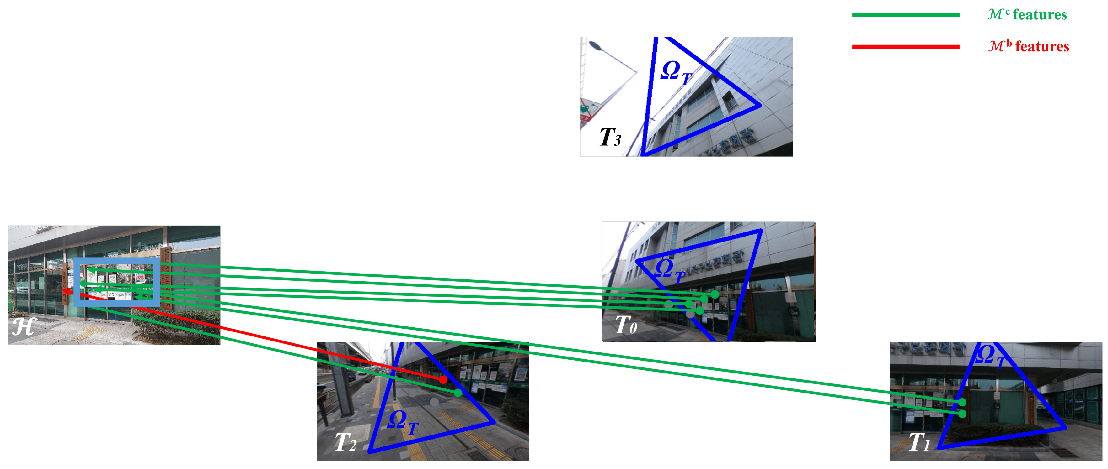
3.4. Tangent Image (TI)-Based Feature Extraction-Matching

Each TI T has a visible region ${\mathsf{\Omega }}_T$ whose distortion level is considered lower than the outside [10] (see Figure 2c). The visibility region ${\mathsf{\Omega }}_T$ is a region in the TI T that covers the icosahedron face $\mathcal{F}$. We perform feature extraction-matching between TIs and the HPI using the ${\mathsf{\Omega }}_T$ region. The ${\mathsf{\Omega }}_T$ forms a triangle mask on the TI. We use the triangle mask as a feature extraction mask for the TI; we do not use the mask for the HPI feature extraction. We perform feature matching between the TI and the HPI using the extracted features. We get the resulting matched features inside the ${\mathsf{\Omega }}_T$. We then reproject the matched features from the neighboring TIs to obtain matched features outside region ${\mathsf{\Omega }}_T$ (see Figure 3).

Figure 3 illustrates an example of feature extraction-matching between a main tangent image (MTI) $T_m$ and the HPI. We first perform feature extraction-matching between MTI and HPI. The process will result in matched features shown as a yellow dashed line in the figure. In addition, we also perform the feature extraction-matching between the HPI and N number of the neighbor tangent images (NTI) $T_{mn}$, where $n=1,2,\dots N$. The feature extraction-matching result in matched features shown in red, blue, and green dashed lines for $T_{m1},T_{m2}$, and $T_{m3}$ respectively. We finally map the features from each NTI coordinate onto MTI coordinate (shown in red, blue, and green straight line for $T_{m1},T_{m2}$, and $T_{m3}$ respectively) using the procedure explained in Section 3.3. We define the total matched features obtained (including the ones reprojected from NTI) in the MTI as the accumulative matched features (AMF).

4. Planar-Equirectangular Image Stitching

Figure 4 shows the three-steps pipeline for our planar-equirectangular image stitching process. First, we detect the ROI position on the EI. The step tries to find the ROI appearance depicted by the HPI input on the EI input. The output from this step will result in an ROI-TI whose appearance is similar to the ROI depicted by the HPI input. Second, we implement the feature extraction-matching between the ROI-TI and the HPI. The step results in ROI-TI and HPI feature matching pairs. Third, we carry out the image alignment between the ROI-TI and the HPI. The step aligns, then blends the HPI. It then processes the blended HPI into two separate ways: (1) directly stitch the blended HPI onto the ROI-TI, and (2) remaps the blended HPI back to equirectangular coordinate through TI-EI mapping procedure using ROI-TI coincident point $C_{ROI}$ (see Section 3.3) then stitches it with EI. The first way will result in a high angular resolution ROI tangent image (HROI-TI); the second way will result in a high angular resolution ROI EI (HROI-EI).

4.1. ROI Detection

We divide the ROI detection into two steps: (1) ROI-TI searching and (2) ROI-TI refinement. The first step aims to pick the closest TI to the ROI: the ROI-TI. The second step refines the ROI-TI position (i.e., coincident point $C_{ROI}$) closer to the true ROI.

4.1.1. ROI Tangent Image (ROI-TI) Searching

As we do not have any prior information about the ROI position on the EI, we need to perform the feature extraction-matching for the whole EI region. Therefore, we use icosahedron with subdivision level $b=0$ (i.e., base-level icosahedron). The lowest b value will generate the smallest number of TIs to represent the whole EI. Thus, it allows for the fastest feature extraction-matching between the HPI and all generated TIs.

We use ORB [25] to extract features from both images quickly. Despite its fast performance, ORB has lower accuracy than other commonly used feature extractors [28] for feature matching tasks. Therefore, we use the grid-based motion statistics (GMS) [12] to improve the accuracy. The GMS is used after the Brute-Force (BF) feature matching process. It identifies correct matches (i.e., true matches) among the feature matching results. We use the identified true matches from the GMS as the final feature matching result.

Precisely, we first generate all possible TIs using the base-level icosahedron. As there are 20 icosahedron faces on the base level, we will obtain a total of 20 TIs. We iterate all 20 TIs $T_m$ and perform the feature reprojection described in Section 3.4 to gather the AMF for each $T_m$ and the HPI. We use the ORB feature extractor, BF feature matcher, and GMS during the process. After we finish iterating the TIs, we will obtain AMF for all 20 TIs.

We employ a coarse-to-fine approach to pick the ROI-TI among the 20 TIs. We first eliminate false TIs from the list of candidates. We define the false TIs as TIs whose false matches value are high. Figure 5 illustrate the process of detecting the false TIs. We expect that FTI has low AMF despite having a high feature number by itself. The tangent images $T_1$ in Figure 5 exhibit such characteristics. Although $T_1$ has high self feature matches, the corresponding NTIs (i.e., $T_{11},T_{12}$, and $T_{13}$) have low feature matches with the HPI. The overall combination will result in low AMF $|{\mathcal{M}}_1|$ for the $T_1$ (shown by red lines). On the contrary, $T_0$ has high AMF $|{\mathcal{M}}_0|$. In addition to having high self feature matches, the corresponding NTI (i.e., $T_{01},T_{02}$, and $T_{03}$) overall also has high feature matches. The overall combination results in high AMF for $T_0$ (shown by green lines).

The false TI elimination will leave several TI candidates to pick as the ROI-TI. To select the ROI-TI, we first categorize the AMF into two: central AMF ${\mathcal{M}}^c$ and boundary AMF ${\mathcal{M}}^b$. The central AMF means that the corresponding feature is located in the HPI central region. On the contrary, the boundary AMF has the corresponding feature outside the HPI central region. We pick the TI whose central AMF is the highest among the remaining ones and assign it as the ROI-TI. Figure 6 illustrates the process.

4.1.2. ROI Tangent Image (ROI-TI) Refinement

As illustrated in Figure 6, on the HPI side, the central AMF ${\mathcal{M}}^c$ is located in the center (i.e., inside the light blue rectangle). On the contrary, the central AMF on the ROI-TI $T_{ROI}=T_0$ side is closer to the boundary than the center. We expect the centralized ${\mathcal{M}}^c$ position to make the ROI-TI coincident point (on the unit sphere) $C_{ROI}\in S$ closer to the true ROI. We use the central AMF centroid $P_{CAMF}\in T_{ROI}$ as the $C_{ROI}\in S$ projection point. We readjust the $P_{CAMF}$ position iteratively.

We first calculate the centroid of current CFM $P_{CAMF}^0\in T_{ROI}^0$. We then convert the centroid pixel coordinate $P_{CAMF}^0$ to the unit sphere $S_{CAMF}^0\in S$ through Equation (3). We set the $S_{CAMF}^0$ as the new coincident point $C_{ROI}^0$. If the central AMF centroid $P_{CAMF}^0$ is not close enough to the ROI-TI central coordinate, we reproject all matched features through feature reprojection as described in Section 3.3 using $C_{ROI}^0$. We then calculate the central AMF centroid $P_{CAMF}^1$, $S_{CAMF}^1$ and the central AMF centroid error from the center. The process repeats until the central AMF centroid $P_{CAMF}^k$ error is close enough to the center. We use the last $C_{ROI}^k$ to generate the refined ROI-TI. We use the refined ROI-TI as input for the next feature extraction-matching step.

4.2. ROI Feature Extraction-Matching

It is crucial to have the matched features distributed across the overlapping region on the image alignment step. In contrast to the standard planar-planar case, the overlapping region of planar-equirectangular image alignment covers the whole HPI. Therefore, we need to have the matched features to be distributed across the HPI. One way to improve the distribution is to increase the number of the matched features. We propose a new kNN-based GMS matcher to increase the numbers of matched features.

GMS has been capable of increasing the number of matched features [12]. It converts the quantity of matched features to identify the quality matches (i.e., the true matches). Precisely, GMS first divided the image into several grids. It then used the number of similar neighbors inside the image grids to identify the correct features. The similar neighbors were defined as features that: (1) located inside the same image grid, and (2) the corresponding features also located inside the same image grid. The higher the number of similar neighbors, the highest the possibility it contains the correct matches.

The original implementation of GMS used the results from the BF matcher as the input (i.e., BF-based GMS matcher). In this paper, we propose to use the kNN feature matcher as the input (i.e., kNN-based GMS matcher). Different from the BF-based GMS matcher that only used the closest feature correspondence (i.e., 1st correspondence) as the input, the proposed approach uses up to k feature correspondences as the input (i.e., 1st, 2nd, …, kth correspondence). We assume there is a possibility that the correct correspondence is on the 2nd, 3rd, …, kth correspondence. We perform the GMS feature matching iteratively according to the number of k. For every iteration, we switch the correspondence to the next closest (e.g., from 1st to 2nd-closest, or from 2nd to 3rd-closest).

Figure 7 illustrates the first and second iteration of the proposed approach. After performing feature matching between the TI and the HPI beforehand, we initially use the 1st correspondence to perform the GMS matcher. Figure 7a shows the situation before the first iteration. Figure 7b shows the result of the first iteration, with a green line that denotes the GMS output. The red, blue, and orange features are similar neighbors: they are located in the same image grid either for the TI side or the HPI side. Thus, they are identified as correct matches. On the contrary, the yellow feature has correspondence (on the HPI side) on a different grid, thus not sharing similar neighbors. Therefore, we switch the yellow to use the 2nd correspondence for the next iteration. As the 2nd correspondence is also located on the same grid as the other correspondences, the yellow feature shared similar neighbors. We repeat the similar pattern for next 3rd, 4th, … kth correspondences.

To improve the feature matching accuracy, we also need to have a less-distorted visibility region ${\mathsf{\Omega }}_T$ on the TIs. Consequently, we use b value higher than the one used for the ROI detection. We set the $b=1$ for this step. Although higher b will increase the number of TIs generated, we only need to gather the AMF on the ROI-TI. Therefore, we only perform the feature extraction-matching between the HPI with the ROI-TI and its corresponding NTIs (see Section 3.4). We use the matching result for the next image alignment step.

4.3. HVS-Based Image Alignment

Although the TI representation has made it possible to carry out existing planar-planar approaches, several differences are found when stitching the HPI onto the EI. In the planar-planar case, the stitching algorithms were designed for side-by-side images. The alignment constraint only applies for one side (i.e., the overlapping one) of each input image, allowing the other side free. In multiple input images, the transformation model of every input image can also be altered [29]. On the contrary, the planar-equirectangular image stitching attempts to put the HPI to their corresponding ROI on the EI. The EI acts as a template that the form should be fixed, leaving the HPI as the only input to be modified. As the EI also covers the whole HPI region, these situations can lead to alignment-distortion error trade-off due to parallax error.

Figure 8 illustrate this situation. Figure 8a,b are the grid representation of the HPI and the ROI-TI respectively. As the parallax error will cause both views to differ slightly, the feature pairs (i.e., numbered circle on the figure) location on each image will also be different. The differences can cause misalignment in the stitching result. A common way to reduce the misalignment is by providing each vertex a separate model (i.e., local hybrid transformation approach). As shown in Figure 8c, the approaches can reduce the alignment error: the feature pairs (i.e., the same numbered circle) located close to each other on the stitching result. However, the features are located in the whole HPI region, and we can only alter the HPI vertices to minimize the alignment error. These situations make the stitching result central region (i.e., the yellow grid) distorted. The central region distortion can be a problem as our initial goal is to provide a high angular resolution version of the ROI-TI. Naturally, the focused object is located in the central of the ROI-TI. Thus, the distortion around the central region can be displeasing.

Figure 8e illustrates the situation when we only want to focus on the central region. A simple way to preserve the central region is by only focusing on the alignment error minimization on the central and using the global transformation model for the whole vertices. This way, the distortion on the central (thus also the focused object) can be minimized. However, the misalignment on the boundary can be seen clearly (e.g., misalignment between feature no. 8, 9, 10, 15, 16).

To handle this alignment-distortion error trade-off, we proposed an image stitching inspired by the HVS. The HVS has a much greater resolution in the central visual field compared to the boundary [11]. It used the center vision (i.e., foveal vision) to resolve the focused object’s detail resolution. On the other hand, the boundary vision (i.e., peripheral vision) exists mainly to provide low-resolution cues to guide the fovea movements [11]. Therefore, we intend to keep the central region of the stitching result as accurate: well-aligned and less distorted. Likewise, we intend to put the stitching result boundary region as well-aligned, thus not distracting human fovea when inspecting the other EI region.

Mathematically, to align the HPI $\mathcal{H}$ with the ROI-TI $T_{ROI}$, we first divide the HPI $\mathcal{H}$ into a vertices grid $v_k^i\in \mathcal{H}$. We then find the affine (i.e., global) model $H_{aff}$ that map the $v_k^i\in \mathcal{H}$ to the $v_k^f\in T_{ROI}$. In addition, we also find the APAP (i.e., local) $H_{apap}$ model that map the $v_k^i\in \mathcal{H}$ to the $v_k^p\in T_{ROI}$. Finally, we linearly combine the two terms to obtain final $v_k^o\in T_{ROI}$:

$$v_k^o=w{H}_{aff}{v}_k^i+(1-w)H_{apap}{v}_k^i,$$

(4)

$$w=e^{-k{R}^2},$$

(5)

where $k>0$ is user-defined constant and R is distance of vertex $v_k^f\in T_{ROI}$ to the ROI-TI grid central. The global-local weight w will vary depending on the vertex’s distance to the image center. The w is higher for vertices close to the center.

Every vertex $v_k^o$ will have the same $H_{aff}$, serving to keep the objects or straight-line less distorted. We choose affine over homography to represent the global term as it has fewer degrees of freedom (DOG). The HPI and the ROI-TI should have a similar scene; thus, fewer DOG models would afford better regularization.

The w is high on the central region to emphasize the $H_{aff}$ term, making the central region less distorted. On the contrary, w is small on the boundary region to emphasize the $H_{apap}$ term, making the boundary region better align with the ROI-TI boundary. We expected to have an alignment result whose distortion error is small on the central region, and alignment error is small on the boundary region as shown in Figure 8d).

To reduce the noticeable artifacts that occurred on the alignment result boundary region, we perform an image alpha blending on the HPI region beforehand. We then perform two separate processes: (1) directly stitch the aligned HPI onto the ROI-TI, and (2) remaps the aligned HPI back to the equirectangular coordinate through the TI-EI mapping procedure (see Section 3.3) then stitches it with EI. The first process will result in the HROI-TI, and the second process will result in the HROI-EI (see Figure 4).

5. Experiment and Discussion

We performed experiments on the laptop with specifications as follows: Intel(R) Core(TM) i7-9750H, 16 GB RAM, Ubuntu 20.04, six cores, and 12 threads. The laptop also used GeForce RTX 2060 with NVIDIA driver 450.102. For the software side, we used OpenFrameworks (https://github.com/openframeworks/openFrameworks/tree/0.11.0, accessed on 9 April 2021) to provide simplified OpenGL interface; OpenCV (https://github.com/opencv/opencv/tree/4.4.0, accessed on 9 April 2021) for image processing; Eigen for optimization (https://gitlab.com/libeigen/eigen/-/tree/3.3.9, accessed on 9 April 2021); CGAL for creating the icosahedron (https://github.com/CGAL/cgal/releases/tag/releases%2FCGAL-5.0.2, accessed on 9 April 2021).

We took the pictures by putting the We collected 14 equirectangular and 16 high-resolution planar images. There are two EIs paired with two high-resolution planar images for each (i.e., ID no. 4-5 and ID no. 14-15), As a result, we have 16 equirectangular-planar image pairs in total, as shown in Figure 9. We used RICOH THETA V [30] to capture the EIs. To capture the HPIs, we used PTZ Logitecth Pro camera [31] (1 image) and Samsung Galaxy Note 5 [32] (15 images). For the THETA V-the Galaxy Note 5 case, we put the THETA V on top of our head to capture the picture, the Galaxy Note 5 in front of our face. For the THETA V-PTZ Logitech, we put the cameras on a camera rig.

The images captured both seven indoor and outdoor scenes with ROI located on various EI regions. Each equirectangular and high-resolution planar image has $3840\times 1920$ and $1920\times 1080$ original image size respectively. We resize the EIs into $1280\times 640$ and high-resolution planar image into $640\times 360$ for image processing purposes.

We performed experiments for each contribution. We analyzed the results then suggest relevant solutions to address the problems found. We also present the computation times took for each planar-equirectangular image stitching pipeline step. In addition, we briefly explore the possibility of implementing the proposed pipeline in other 360° image formats. We hence organize this section in the following orders:

• KNN-Based GMS Feature Matcher.
• ROI detection.
• Tangent image (TI)-based planar-equirectangular image stitching pipeline.
• HVS-based image alignment.
• Computation time.
• Implementation in other 360° image format.

5.1. KNN-Based Gms Feature Matcher

We experimented with the ROI-TI and the HPI feature matching; we focused on providing higher inliers for the image alignment step. We measured the correct matches number (#inliers), accuracy, and entropy [28] to evaluate the performance. The #inliers denoted how many correct feature matches were detected; accuracy tells how accurate the feature matching was; entropy represents the correct feature match spread level on the ROI-TI. We also showed the inliers relative increase (in percentage) of the proposed KNN-based relative to the BF approach. We identified the correct and wrong feature pairs by manual intervention after the matching.

Table 1. Feature matching result between the ROI tangent image (ROI-TI) and the high-resolution planar image (HPI). We compared the original BF-based GMS Matcher (Original) and the kNN-based GMS Matcher (Proposed). The proposed approach can increase number of inliers (# Inliers) up to $29.0\%$ compared to the original. It also increases the the matched features distribution (Entropy), which is the main purpose of the proposed approach. There is a slight reduction in Accuracy but the value is still high.

ID	# Inliers		Entropy		Accuracy (%)
	Original	Proposed	Original	Proposed	Original	Proposed
1	4127	5107	5.36	5.40	97.9	97.1
2	2755	3625	5.41	5.46	99.6	98.9
3	3112	3971	5.25	5.33	99.5	98.2
4	5249	6497	5.70	5.73	98.4	97.9
5	1228	1784	5.21	5.26	97.7	95.5
6	3009	3922	5.28	5.34	99.2	98.0
7	1698	2294	5.15	5.23	96.8	97.1
8	2432	3234	5.16	5.22	98.9	98.3
9	847	1165	4.10	4.08	97.6	97.7
10	2330	3170	5.09	5.11	96.3	95.2
11	2410	3097	4.88	4.92	99.8	99.5
12	2365	3155	5.49	5.53	99.7	99.2
13	2049	2845	5.25	5.32	90.3	86.3
14	3193	3959	5.41	5.47	92.3	89.5
15	2502	3160	5.18	5.23	98.7	98.5
16	4633	5717	5.35	5.39	98.9	98.7
Avg	2746	3544 (29.0%)1	5.20	5.25	97.6	96.6

¹ The % denotes the relative increase to the BF.

showed improved feature match count (#inliers) detected by using the proposed kNN-based GMS matcher. We could see an increase of inliers up to $29.0\%$ on the # Inliers and Entropy (5.25 vs. 5.20) compared to the original BF-matcher implementation. Although the accuracy was higher for the BF-based GMS matcher (96.6% vs. 97.6%), the proposed kNN-based GMS matcher had already been high (owing to the scene similarity between the ROI-TI and the HPI). This result showed that our proposed kNN-based GMS feature matcher could improve the number and distribution (i.e., entropy) of the feature matches.

We analyzed deeper on the decrease of the accuracy. The decreased means there was also an increase in the number of wrong matches (i.e., outliers) during the $k=2,3,\dots ,K$ iterations. The increase of the inliers and also the outliers made the accuracy pretty much stayed the same.

We believed the cause of the phenomenon was that similar neighbor feature members correspond to the wrong matches. The situation is illustrated in Figure 10. In other words, if the similar neighbors were already correct since the beginning, then the number of the inliers would increase. On the contrary, if the similar neighbors were wrong since the beginning, then the number of the outliers would increase. We concluded that the increase of inliers came from the increase of “correct” similar neighbors feature members; it did not come from the change of the “wrong” similar neighbors to the “correct” similar neighbors. The analysis was in line because entropy could only slightly improve (from 5.20 to 5.25): the new inliers come from the same image grid. The proposed approach was unable to distribute the inliers to the other grids.

Regardless, the experiment showed that switching the correspondence to the next one could increase feature matches. We seek a better way to switch the correspondence (i.e., not merely switch it to the next one). For example, we could incorporate the scale information around similar neighbors to pick the subsequent correspondence.

5.2. ROI Detection

We determine the ground truth ROI position (i.e., coincident point $C_{GT}$) for each image set beforehand. We then measured the angle between the ROI-TI coincident point $C_{ROI}$ and the $C_{GT}$. We used the angle as the error indicator as the coincident points are located on the unit sphere surface (see Section 3.1).

Table 2. ROI detection experiment result. The Angular Error (°) denotes angle difference between the ROI tangent image (ROI-TI) coincident point $C_T$ and the ground truth coincident point $C_{GT}$. The “Initial” represents the angular error between the $C_{ROI}$ and the $C_{GT}$ before the refinement process; the “Refined” represents the angular error between the $C_{ROI}$ and the $C_{GT}$ before the refinement process after the refinement process. The “Refined” error is the final ROI-TI $C_T$ error to $C_{GT}$.

ID	Angular Error (°)		ID	Angular Error (°)
	Initial	Refined		Initial	Refined
1	32.8	8.37	9	10.7	3.24
2	32.8	5.51	10	2.48	1.34
3	6.74	1.18	11	33.1	15.5
4	18.6	0.942	12	17.3	12.6
5	9.94	1.54	13	19.1	9.16
6	18.2	5.45	14	10.0	6.22
7	14.9	3.29	15	20.6	6.54
8	16.8	5.01	16	13.4	5.58
Avg	17.3	5.72

summarized the ROI detection experiment results. The “Initial” columns denoted $C_{ROI}$ error to the $C_{GT}$ after the ROI-TI searching step;the “Refined” columns denoted $C_{ROI}$ error to the $C_{GT}$ after the refinement step. On average, the ROI-TI searching step had the $C_{ROI}$ deviated around 17.3° from the $C_{GT}$. The refinement could reduce the error closer up to 5.72° on average. It can be seen that the orientation error was below 15° on 15 of 16 image sets, with 14 of them below 10°. The result showed that the detection picked the correct closest face. Therefore, the follow-up refinement could reduce the orientation error further.

5.3. Tangent Image (TI)-Based Planar-Equirectangular Stitching Pipeline

We evaluated the proposed TI-based planar-equirectangular image stitching pipeline performance. We compared the proposed method to the existing planar-planar image stitching pipeline. In other words, we checked whether the intermediate transition from EI to the ROI-TI could reduce the undesired distortion on the stitching result compared to stitch the HPI onto the EI directly. It is important to note that we mainly focused on evaluating the image alignment step, leaving other stitching pipeline steps untouched. Both methods would use the same feature pairs and only differ on which coordinate was used to represent the EI features. The TI-based approach used the ROI-TI coordinate, while the planar-planar image alignment approach used the EI coordinate. We used the existing affine transformation model for both and performed the alpha blending afterward.

Figure 11 showed the results. On image no. 1, we see that both approaches resulted in similar results either for the HROI-EI or for the HROI-TI. The results were as expected because the ROI was located about the center region of the EI. This area had low spherical image distortion; thus, the planar-planar image stitching algorithm could work well.

Images no. 2 and no. 3 in Figure 11 show that the planar-planar image alignment caused significant distortion. The ROI of image no. 3 located further from the central compared to the no. 2. The stitching results were more distorted as the spherical distortion was higher further from the EI central region. The worst result was shown in image no. 4, where most of the ROI was located on the EI polar region. This region had the strongest distortion compared to the others. We could see how the output image of planar-planar image alignment could not even be recognized. On the contrary, images no. 2, 3, and 4 could still be recognized fine on the proposed TI-based one. The result showed that, as opposed to the less-distorted wide FOV image where the typical planar-planar image stitching can still work [21], the distortion on the EI was too strong to give a good image stitching result.

5.4. HVS-Based Image Alignment

As a preprocessing step, we divided the HPI into grids of $33\times 19$ vertices. We used an ellipse mask to perform alpha blending on the HPI. We then stitched the blended alpha to the ROI-TI, which resulted in HROI-TI. We focused on evaluating the HROI-TI during this experiment.

As the proposed approach is naturally a combination of affine and APAP, we also used the affine and APAP model as the comparator. Moreover, as the proposed HVS-based alignment approach attempted to address the alignment and distortion error on the stitching result, we used both alignment and distortion error as our evaluation metric. We showed both errors qualitatively through image inspection; quantitatively through alignment and distortion error calculation.

5.4.1. Qualitative Measurement

Figure 12 showed the results of this experiment. We outlined our qualitative inspection as red, yellow, and green for “bad”, “medium”, and “good” results. The qualitative inspections are based on the distortion and misalignment that occurred on the outlined parts. The ground truths are obtained from the ROI-TI: we want to have a stitching result that provides the high-resolution version of the ROI-TI without having misalignment along the boundary and without distorting them (especially around the central region).

In image no. 1, we can see that affine transformation suffered misalignment along the boundary. On the contrary, APAP and the proposed (i.e., HVS-based) approach can align pretty well around the region. Image no. 2 showed more complicated situations. The ROI region roughly consisted of multiple planes. For example, object no. 4 (i.e., focused object) was located on a separate plane compared to objects no. 1 and no. 2. The affine transformation could align with an object no. 4 pretty well but suffer from misalignment on other objects. On the other hand, APAP could align objects no. 1, no. 2, no. 3, and no. 5, whose located around the boundary. However, object no. 4 was distorted. Our proposed method could align all the objects as they adopt affine factor on the central region and APAP factor on the boundary region.

Image no. 3 had a similar result. The affine method could keep the object no. 4 (i.e., focused object) boundary shape straight. However, it misaligned the other objects. The APAP method could align the boundary better even though the scattered and uneven objects make it harder to align them perfectly. The proposed method gets a similar result as the APAP but can preserve the object no. 4 shapes better. Image no. 4 also behaves similarly as the no. 3. However, as the APAP and affine cannot align object no. 3, the proposed method cannot align object no. 3. The case shows the fail-case of our method.

One way to improve the alignment during the boundary is to provide a distributed alignment on the boundary. The lack of matched features around the ROI-TI can be seen on object no. 3 on Image no. 4. We plan to improve our kNN-based feature matching approach to add new the similar neighbors around the boundary. Furthermore, the failure to perfectly align the boundary objects can be essential or not. The use of widescreen or HMD to observe the stitching result can affect the importance of perfect boundary region alignment, as long as the crucial focused object can be viewed accurately in high-resolution. The premise is in line with our HVS-based assumption to generate the stitching result. In the future, we would like to perform a user study to test whether our image alignment algorithm could provide adequate stitching results.

Nevertheless, distortion found on the focused objects can be displeasing. The situation occurred due to the various size of the focused objects. For instance, object no. 4 on image no. 3 (i.e., the keyboard) is horizontally elongated, while object no. 4 on image no. 4 (i.e., the street sign) is vertically elongated. The problems can potentially be solved if we can adjust the global-local weight w accordingly. Currently, the global-local weight w (see Equation (4) is still decided manually by the user. Object recognition [33] or line detection [34] to find the focused object region can automatically adjust global-local weight w. We can group the vertices according to objects detected in the region. We then use the same local model term for vertices that belong to the same objects.

5.4.2. Quantitative Measurement

To calculate the alignment error $e_{align}$, we first calculated the root-mean-squared error (RMSE) between AMF pairs. We used the inspected approaches (i.e., the HVS-based, the APAP, or the Affine) to transform the matched features from the HPI coordinate to the ROI-TI coordinate. We then found the RMSE between the transformed features with their correspondences in the ROI-TI. We set the RMSE as the alignment error $e_{align}$ [14].

To determine the distortion error $e_{distort}$, we first calculated the 2D rigid-body similarity constraint error [20] of the stitching result vertices. As we only focused on central distortion error, we only calculated the vertices located nearby the image center. To decide it, we assigned an image grid whose size is $3\times 3$ distributed evenly inside the image. We described the central vertices as the vertices whose closest grid is the center grid. We averaged these central vertices similarity errors and used them as the distortion error $D_{err}$.

In addition, we also defined aggregated alignment-distortion $e_{aggregate}$ for APAP P, Affine F, and the proposed HVS-based V comparison:

$$\left\{\alpha \in \mathbb{A}|e_{aggregate}\left(\alpha \right)=0.5{\displaystyle \frac{e_{align}\left(\alpha \right)}{{\sum }_{\gamma \in \mathbb{A}}{e}_{align}\left(\gamma \right)}}+0.5{\displaystyle \frac{e_{distort}\left(\alpha \right)}{{\sum }_{\gamma \in \mathbb{A}}{e}_{distort}\left(\gamma \right)}}\right\},$$

(6)

where $\mathbb{A}=\{P,F,V\}$. The equation is a simple approach to aggregate the relative error of both $e_{align}$ and $e_{distort}$. As our proposed image alignment method is trying to find the trade-off between $e_{align}$ and $e_{distort}$, we expected that our proposed method would not often be shown the best on both criteria. Therefore, we intended to use this metric to show the overall performance of our proposed method in compensating both $e_{align}$ and $e_{distort}$. We made following hypothesis:

• $e_{align}$ on proposed method (V) is lower than affine (F) but higher than APAP (P): $e_{align}\left(F\right)>e_{align}\left(V\right)>e_{align}\left(P\right)$
• $e_{distort}$ on proposed method (V) is lower than APAP (P) but higher than affine (F): $e_{distort}\left(P\right)>e_{distort}\left(V\right)>e_{distort}\left(F\right)$
• $e_{aggregate}$ on proposed method (V) is lower than both APAP (P) and affine (F): $e_{aggregate}\left(P\right)>e_{aggregate}\left(V\right)$ and $e_{aggregate}\left(F\right)>e_{aggregate}\left(V\right)$

Table 3. Results for the image alignment step between the ROI tangent image (ROI-TI) with the high-resolution planar image (HPI). We compared the image alignment step output of the Proposed (V) approach with existing Affine $\left(F\right)$ and APAP $\left(P\right)$ approaches. Most of results follow the alignment error hypotheses $e_{align}\left(F\right)>e_{align}\left(V\right)>e_{align}\left(P\right)$ (11 of 16); distortion error hypotheses $e_{distort}\left(P\right)>e_{distort}\left(V\right)>e_{distort}\left(F\right)$ (12 of 16); alignment-distortion error hypotheses $e_{aggregate}\left(P\right)>e_{aggregate}\left(V\right),e_{aggregate}\left(F\right)>e_{aggregate}\left(V\right)$ (12 of 16). Overall, the proposed approach shows the lowest aggregated alignment-distortion error $e_{aggregate}$ (i.e., 0.61) compared to Affine (0.72) and APAP (0.67).

ID	APAP $\left(\mathit{P}\right)$	Affine $\left(\mathit{F}\right)$	Proposed $\left(\mathit{V}\right)$	Hypotheses	ID	APAP $\left(\mathit{P}\right)$	Affine $\left(\mathit{F}\right)$	Proposed $\left(\mathit{V}\right)$	Hypotheses
Alignment Error $e_{align}$ (pixel)
1	3.54	4.95	3.59	TRUE	9	5.68	6.91	6.15	TRUE
2	5.96	11.2	7.65	TRUE	10	6.85	9.78	6.70	FALSE
3	6.26	8.63	6.93	TRUE	11	8.73	15.4	9.80	TRUE
4	5.76	6.13	5.47	FALSE	12	6.06	14.3	7.66	TRUE
5	6.95	10.3	7.25	TRUE	13	7.83	24.6	8.83	TRUE
6	6.73	11.7	6.96	TRUE	14	7.05	18.7	9.52	TRUE
7	6.16	7.70	6.04	FALSE	15	3.76	4.20	3.76	FALSE
8	3.33	3.77	3.28	FALSE	16	4.99	5.98	5.02	TRUE
Avg ${}^1$	5.98	10.3	6.54	11 of 16
Distortion Error $e_{distort}$ (pixel)
1	0.98	0.78	0.82	TRUE	9	2.80	2.49	2.65	TRUE
2	0.79	0.73	0.75	TRUE	10	1.23	0.99	1.01	TRUE
3	1.52	1.12	1.23	TRUE	11	1.32	0.47	0.91	TRUE
4	0.46	0.67	0.56	FALSE	12	0.92	0.60	0.73	TRUE
5	0.63	0.43	0.42	FALSE	13	1.52	0.91	1.00	TRUE
6	1.11	0.52	0.72	TRUE	14	1.59	1.58	1.70	FALSE
7	0.78	0.77	0.70	FALSE	15	0.36	0.31	0.32	TRUE
8	0.67	0.37	0.43	TRUE	16	1.08	0.56	0.66	TRUE
Avg ${}^1$	1.11	0.83	0.91	12 of 16
Alignment-Distortion Error $e_{aggregate}$
1	0.67	0.71	0.62	TRUE	9	0.66	0.68	0.66	FALSE
2	0.59	0.78	0.64	FALSE	10	0.68	0.72	0.60	TRUE
3	0.68	0.68	0.64	TRUE	11	0.75	0.63	0.62	TRUE
4	0.61	0.75	0.64	FALSE	12	0.62	0.78	0.60	TRUE
5	0.71	0.71	0.58	TRUE	13	0.63	0.86	0.50	TRUE
6	0.74	0.68	0.58	TRUE	14	0.53	0.85	0.62	FALSE
7	0.66	0.73	0.62	TRUE	15	0.68	0.67	0.65	TRUE
8	0.78	0.61	0.61	TRUE	16	0.78	0.62	0.60	TRUE
Avg ${}^1$	0.67	0.72	0.61	12 of 16

${}^1$ Average of hypotheses means a count of TRUE value.

summarized the result for this experiment. Overall, the results of the experiment followed our three hypotheses with some exceptions. Most of the time, the $e_{aggregate}$ could show that our proposed method is best (12 of 16 cases). However, this metric alone can give a different interpretation when compared with the other two hypotheses. For instance, ID no. 5 showed that the proposed approach followed both alignment and distortion error hypotheses yet gave FALSE results overall. On the contrary, this metric gave TRUE results on image ID no. 7 despite violating both alignment and distortion error hypotheses.

The ID no. 5, 7, 8, 10, and 15 showed that our method has the lowest $e_{align}$ compared to others. These are examples of ideal cases where our proposed method could get the lowest alignment error as it took the best factor on both central and boundary regions. On the central, the affine factor contributed more to our proposed method, while on the boundary, the APAP factor contributed more. These cases showed that the affine factor could align the central region well even though it has a high $e_{align}$ on the boundary. Alignment during the central-boundary transition also works well on our proposed method resulted in the lowest $e_{align}$.

A similar reason can also hold on $e_{distort}$ case. As we measured only the central distortion, we got a similar distortion error between the proposed method and the affine model. The transition between central to boundary region could only cause slight differences, which could be positive (lower $e_{distort}$) or negative (higher $e_{distort}$) effect. The ID no. 6 and 7 showed that our method has the lowest $e_{distort}$. On the contrary, image ID no. 14 showed our method has the highest $e_{distort}$.

On the proposed image alignment, we relied on the affine model characteristics property to keep the shape in the ROI region (i.e., to preserve the ROI region similarity). We did not explicitly add a similarity constraint to the equation [18]. Therefore, there are possibilities that the affine model had a higher distortion error compared to the APAP model, such as shown on image ID no. 5.

5.5. Computation Time

Table 4. Computation time for each planar-equirectangular image stitching pipeline steps (in seconds). The majority of the computation times were occurred on the ROI detection step (43.6%), followed by alignment (39.4%) and ROI feature extraction-matching (17.0%), respectively.

ID	ROI Detection (s)	ROI Extraction-Matching (s)	Alignment (s)
1	3.47	0.84	2.60
2	3.71	1.12	2.99
3	2.06	1.26	2.94
4	4.81	1.03	4.16
5	3.25	0.78	2.56
6	2.84	0.59	2.82
7	2.95	1.61	2.42
8	2.12	1.69	2.19
9	1.98	2.30	1.64
10	3.06	1.54	2.55
11	1.39	1.09	2.03
12	2.05	1.50	3.57
13	3.08	1.01	2.75
14	4.90	1.01	3.52
15	4.92	0.69	2.76
16	2.57	1.09	2.87
Avg ${}^1$	3.07 (43.6%)	1.20 (17.0%)	2.77 (39.4%)

¹ The % denotes the percentage of the computation time relative to the overall steps.

showed that most of the processing occurred during the ROI detection step. The ROI detection step also took much longer than the ROI-TI feature extraction matching step. We look deeper at both steps and found that most computation time was used to extract the features from generated TIs. The ROI detection used $b=0$ to generate 20 TIs. It extracted the features from all available TIs. On the contrary, the ROI feeature extraction-matching step used $b=1$. Although generated 80 TIs in total, the step did not extract the features from all TIs. It only extracted features at ROI-TI and its neighbors, which is around 13 TIs in total. Furthermore, the visibility region ${\mathsf{\Omega }}_T$ was higher for $b=0$, making the triangle mask for feature extraction wider. We believe that differentiating and adjusting some of the ORB feature extractor hyperparameters could solve the problem.

The image alignment step also took a similar computation time as the ROI detection. We look deeper into the image alignment and found that The computation time was mainly used to count the local $H_{apap}$ term. We think of two ways to solve the computation time problem. First, we would like to use a faster optimization solver library than Eigen to compute the models. Second, we would like to vary the HPI grid vertices number. On the preliminary test, we used $17\times 10$ vertices and applied the similarity constraint explicitly. This setting is quite similar to applied on [18]. However, as the planar-equirectangular image stitching overlapping region is bigger than the typical planar-planar image stitching, we found that the vertices size was inadequate. We are still figuring out the best setting for the vertices.

5.6. Implementation in Other 360° Image Format

Although we specifically designed our system to handle the 360° image in equirectangular format, the TI can be extended to handle the other formats. A straightforward way is by changing the equirectangular to unit sphere mapping (see Equation (1)) according to each format model. For example, we can use the unified spherical model (USM) [35] to map the fisheye or catadioptric image onto the unit sphere [36,37].

Besides, the use of other image formats than EI can be beneficial for some cases. Precisely, the EI captured by the RICOH THETA V initially captures the image in the dual-fisheye format. The camera internally stitches the two fisheye images to produce the EI. The EI then suffered from the stitching artifacts found on the two fisheye images overlapping region. As the planar-equirectangular image stitching relies on the reliability of the EI image, the artifacts on the boundary region can reduce the performance (e.g., the feature extraction-matching or the image alignment performance) when stitching the images around the boundary.

6. Conclusions

We introduce a planar-equirectangular image stitching algorithm that places the HPI onto their corresponding ROI region on the EI. The proposed method includes: (1) TI-based planar-equirectangular stitching pipeline, (2) kNN-based GMS feature matching, (3) planar-equirectangular image ROI detection, and (4) HVS-based image alignment.

The TI generation in the stitching pipeline could mitigate the strong spherical image distortion on the EI. It is possible to employ existing planar-based feature extraction-matching and image alignment on the TIs. The proposed kNN-based GMS feature matching is implemented to increase the feature match inliers and entropy. The increase of inliers would make the matched features covered a wider overlapping region than typical planar-planar image stitching. The feature extraction-matching result is then used to conduct ROI detection and HVS-based image alignment. The ROI detection algorithm performs a coarse-to-fine searching process on the base-level TI: (1) find the ROI-TI then (2) refine the ROI-TI position vector incrementally. The image alignment is next conducted between the ROI-TI and the HPI. As the parallax error can instigate alignment-distortion error trade-off when stitching the planar image onto the equirectangular one, the proposed HVS-based alignment yields a less distorted central region while minimizing the boundary mismatch. The approach keeps the focused object on the central region (e.g., rigid structure or line) less distorted while placing the HPI on the EI ROI with slight misalignment.

We conducted a qualitative and quantitative experiment on the collected dataset and got the following results: (1) compared to original BF-based GMS feature matching, the kNN-based approach showed an increase of feature matches up to 29.0% and higher entropy value (5.25 vs. 5.20), (2) the ROI detection algorithm could find the ROI direction vector up to 5.72° error on average, (3) less distorted stitching result when using TI-based compared to existing planar-planar image stitching, and (4) the HVS-based image alignment gave lowest aggregated alignment-distortion error over affine and APAP method (0.61 vs. 0.72 vs. 0.67).

The experiments also showed several shortcomings of our methods. First, the kNN-based feature matching could not provide a noticeable improvement on the correct matches spreads level (i.e., entropy value). Second, the ROI detection algorithm could not improve the AMF entropy significantly as they only increase the amount of existing similar neighbor grid members: not adding new similar neighbor grids. A better way to switch correspondences could potentially increase entropy and accuracy. Third, the calculation of ROI orientation still consumed significant computational time compared to other steps. An adjustment on the ORB feature extractor hyperparameters could potentially solve the issue. Fourth, the best combination of global affine and local homography model still required user intervention as the focused object sizes can be varied. Additional object recognition or line detection step to automatically adjust the weight can be explored in the future. Another way is to add the similarity constraints to improve the focus object shape through a faster optimization library or a parallel processing algorithm.

We also would like to adopt more advanced seam-driven image stitching for future works [38,39]. We believe such a method will make a smoother stitching result boundary though we have to consider the increased computation time and reduced high-resolution region possibility. Furthermore, we would like to deploy our algorithm on the VR headset. We want to perform a user study to test whether our image alignment algorithm could provide adequate stitching results.

References

- Sumikura, S.; Shibuya, M.; Sakurada, K. OpenVSLAM: A Versatile Visual SLAM Framework. In Proceedings of the 27th ACM International Conference on Multimedia (MM ’19); ACM: New York, NY, USA, 2019; pp. 2292–2295. [Google Scholar] [CrossRef] [Green Version]
- Barmpoutis, P.; Stathaki, T.; Dimitropoulos, K.; Grammalidis, N. Early Fire Detection Based on Aerial 360-Degree Sensors, Deep Convolution Neural Networks and Exploitation of Fire Dynamic Textures. Remote Sens. 2020, 12, 3177. [Google Scholar] [CrossRef]
- Jokela, T.; Ojala, J.; Väänänen, K. How People Use 360-Degree Cameras. In Proceedings of the 18th International Conference on Mobile and Ubiquitous Multimedia (MUM ’19); Association for Computing Machinery: New York, NY, USA, 2019. [Google Scholar] [CrossRef]
- Pelham, S. OHIO Students Use 360-Degree Videos to Document Daily Life during COVID-19. 2020. Available online: https://www.ohio.edu/news/2020/04/ohio-students-use-360-degree-videos-document-daily-life-during-covid-19 (accessed on 9 April 2021).
- Times, T.N.Y. Introducing the Daily 360 from The New York Times. The New York Times. 2016. Available online: https://www.nytimes.com/2016/11/01/nytnow/the-daily-360-videos.html (accessed on 9 April 2021).
- Ferdig, R.E.; Kosko, K.W. Implementing 360 Video to Increase Immersion, Perceptual Capacity, and Teacher Noticing. TechTrends 2020, 64, 849–859. [Google Scholar] [CrossRef]
- Syawaludin, M.F.; Lee, M.; Hwang, J.I. Foveation Pipeline for 360° Video-Based Telemedicine. Sensors 2020, 20, 2264. [Google Scholar] [CrossRef] [PubMed]
- Szeliski, R. Image Alignment and Stitching: A Tutorial. Found. Trends Comput. Graph. Vis. 2006, 2, 1–104. [Google Scholar] [CrossRef]
- Lyu, W.; Zhou, Z.; Chen, L.; Zhou, Y. A survey on image and video stitching. Virtual Real. Intell. Hardw. 2019, 1, 55–83. [Google Scholar] [CrossRef]
- Eder, M.; Shvets, M.; Lim, J.; Frahm, J.M. Tangent Images for Mitigating Spherical Distortion. In Proceedings of the IEEE/CVF Conference on Computer Vision and Pattern Recognition (CVPR), Seattle, WA, USA, 14–19 June 2020. [Google Scholar]
- Johnson, J. Chapter 6—Our Peripheral Vision is Poor. In Designing with the Mind in Mind; Johnson, J., Ed.; Morgan Kaufmann: Boston, MA, USA, 2010; pp. 65–77. [Google Scholar] [CrossRef]
- Bian, J.W.; Lin, W.Y.; Liu, Y.; Zhang, L.; Yeung, S.K.; Cheng, M.M.; Reid, I. GMS: Grid-Based Motion Statistics for Fast, Ultra-robust Feature Correspondence. Int. J. Comput. Vis. 2020, 128, 1580–1593. [Google Scholar] [CrossRef] [Green Version]
- Lin, C.; Pankanti, S.U.; Ramamurthy, K.N.; Aravkin, A.Y. Adaptive as-natural-as-possible image stitching. In Proceedings of the 2015 IEEE Conference on Computer Vision and Pattern Recognition (CVPR), Boston, MA, USA, 7–12 June 2015; pp. 1155–1163. [Google Scholar] [CrossRef] [Green Version]
- Zaragoza, J.; Chin, T.; Tran, Q.; Brown, M.S.; Suter, D. As-Projective-As-Possible Image Stitching with Moving DLT. IEEE Trans. Pattern Anal. Mach. Intell. 2014, 36, 1285–1298. [Google Scholar] [CrossRef] [PubMed] [Green Version]
- Brown, M.; Lowe, D.G. Recognising Panoramas. In Proceedings of the Ninth IEEE International Conference on Computer Vision, Nice, France, 13–16 October 2003; Volume 2, pp. 1218–1225. [Google Scholar]
- Brown, M.; Lowe, D. Automatic Panoramic Stitching Using Invariant Features. Int. J. Comput. Vis. 2007, 74, 59–73. [Google Scholar] [CrossRef] [Green Version]
- Gao, J.; Kim, S.J.; Brown, M.S. Constructing image panoramas using dual-homography warping. In Proceedings of the CVPR 2011, Colorado Springs, CO, USA, 20–25 June 2011; pp. 49–56. [Google Scholar] [CrossRef]
- Chen, Y.S.; Chuang, Y.Y. Natural Image Stitching with the Global Similarity Prior. In Computer Vision—ECCV 2016; Leibe, B., Matas, J., Sebe, N., Welling, M., Eds.; Springer International Publishing: Cham, Switzerland, 2016; pp. 186–201. [Google Scholar]
- Lin, K.; Jiang, N.; Cheong, L.F.; Do, M.; Lu, J. SEAGULL: Seam-Guided Local Alignment for Parallax-Tolerant Image Stitching. In European Conference on Computer Vision; Springer: Cham, Switzerland, 2016; Volume 9907, pp. 370–385. [Google Scholar] [CrossRef]
- Igarashi, T.; Moscovich, T.; Hughes, J.F. As-Rigid-as-Possible Shape Manipulation. ACM Trans. Graph. 2005, 24, 1134–1141. [Google Scholar] [CrossRef]
- Dornaika, F.; Elder, J.H. Image Registration for Foveated Panoramic Sensing. ACM Trans. Multimed. Comput. Commun. Appl. 2012, 8. [Google Scholar] [CrossRef]
- Dong, Y.; Pei, M.; Zhang, L.; Xu, B.; Wu, Y.; Jia, Y. Stitching Videos from a Fisheye Lens Camera and a Wide-Angle Lens Camera for Telepresence Robots. arXiv 2019, arXiv:1903.06319. [Google Scholar]
- Eder, M.; Frahm, J.M. Convolutions on Spherical Images. In Proceedings of the IEEE/CVF Conference on Computer Vision and Pattern Recognition (CVPR) Workshops, Long Beach, CA, USA, 16–20 June 2019. [Google Scholar]
- Zhao, Q.; Feng, W.; Wan, L.; Zhang, J. SPHORB: A Fast and Robust Binary Feature on the Sphere. Int. J. Comput. Vis. 2015, 113, 143–159. [Google Scholar] [CrossRef]
- Rublee, E.; Rabaud, V.; Konolige, K.; Bradski, G. ORB: An efficient alternative to SIFT or SURF. In Proceedings of the 2011 International Conference on Computer Vision, Barcelona, Spain, 6–13 November 2011; pp. 2564–2571. [Google Scholar] [CrossRef]
- Coxeter, H.S.M. Introduction to Geometry; Wiley: New York, NY, USA, 1969. [Google Scholar]
- Mackay, A.L. To find the largest sphere which can be inscribed between four others. Acta Crystallogr. Sect. A 1973, 29, 308–309. [Google Scholar] [CrossRef]
- Heinly, J.; Dunn, E.; Frahm, J.M. Comparative Evaluation of Binary Features. In Computer Vision—ECCV 2012; Fitzgibbon, A., Lazebnik, S., Perona, P., Sato, Y., Schmid, C., Eds.; Springer: Berlin/Heidelberg, Germany, 2012; pp. 759–773. [Google Scholar]
- Chang, C.; Sato, Y.; Chuang, Y. Shape-Preserving Half-Projective Warps for Image Stitching. In Proceedings of the 2014 IEEE Conference on Computer Vision and Pattern Recognition, Columbus, OH, USA, 23–28 June 2014; pp. 3254–3261. [Google Scholar] [CrossRef] [Green Version]
- RICOH. Product | RICOH THETA. 2018. Available online: https://theta360.com/en/about/theta/ (accessed on 9 April 2021).
- Logitech. Enable Every Room. Enable Every Person. Available online: https://www.logitech.com/assets/64494/vc-whitepaper.pdf (accessed on 9 April 2021).
- Samsung Galaxy Note 5—The Official Samsung Galaxy Site. Available online: https://www.samsung.com/global/galaxy/galaxy-note5/ (accessed on 9 April 2021).
- Herrmann, C.; Wang, C.; Bowen, R.S.; Keyder, E.; Zabih, R. Object-Centered Image Stitching. In Computer Vision—ECCV 2018; Ferrari, V., Hebert, M., Sminchisescu, C., Weiss, Y., Eds.; Springer: Cham, Switzerland, 2018; pp. 846–861. [Google Scholar]
- Xiang, T.Z.; Xia, G.S.; Bai, X.; Zhang, L. Image stitching by line-guided local warping with global similarity constraint. Pattern Recognit. 2018, 83, 481–497. [Google Scholar] [CrossRef] [Green Version]
- Mei, C.; Rives, P. Single view point omnidirectional camera calibration from planar grids. In Proceedings of the IEEE International Conference on Robotics and Automation, Rome, Italy, 10–14 April 2007; pp. 3945–3950. [Google Scholar] [CrossRef] [Green Version]
- Rameau, F.; Demonceaux, C.; Sidibé, D.; Fofi, D. Control of a PTZ Camera in a Hybrid Vision System. In Proceedings of the International Conference on Computer Vision Theory and Applications (VISAPP), Lisbon, Portugal, 5–8 January 2014; Volume 3, pp. 397–405. [Google Scholar]
- Courbon, J.; Mezouar, Y.; Martinet, P. Evaluation of the unified model of the sphere for fisheye cameras in robotic applications. Adv. Robot. 2012, 26, 947–967. [Google Scholar] [CrossRef] [Green Version]
- Zhang, F.; Liu, F. Parallax-Tolerant Image Stitching. In Proceedings of the 2014 IEEE Conference on Computer Vision and Pattern Recognition, Columbus, OH, USA, 23–28 June 2014; pp. 3262–3269. [Google Scholar] [CrossRef] [Green Version]
- Lin, K.; Jiang, N.; Cheong, L.; Do, M.N.; Lu, J. SEAGULL: Seam-Guided Local Alignment for Parallax-Tolerant Image Stitching. In Computer Vision—ECCV 2016—14th European Conference, Amsterdam, The Netherlands, 11–14 October 2016, Proceedings, Part III; Leibe, B., Matas, J., Sebe, N., Welling, M., Eds.; Lecture Notes in Computer Science; Springer: Cham, Switzerland, 2016; Volume 9907, pp. 370–385. [Google Scholar] [CrossRef]