Sigmoidal NMFD: Convolutional NMF with Saturating Activations for Drum Mixture Decomposition

Abstract

In many types of music, percussion plays an essential role to establish the rhythm and the groove of the music. Algorithms that can decompose the percussive signal into its constituent components would therefore be very useful, as they would enable many analytical and creative applications. This paper describes a method for the unsupervised decomposition of percussive recordings, building on the non-negative matrix factor deconvolution (NMFD) algorithm. Given a percussive music recording, NMFD discovers a dictionary of time-varying spectral templates and corresponding activation functions, representing its constituent sounds and their positions in the mix. We observe, however, that the activation functions discovered using NMFD do not show the expected impulse-like behavior for percussive instruments. We therefore enforce this behavior by specifying that the activations should take on binary values: either an instrument is hit, or it is not. To this end, we rewrite the activations as the output of a sigmoidal function, multiplied with a per-component amplitude factor. We furthermore define a regularization term that biases the decomposition to solutions with saturated activations, leading to the desired binary behavior. We evaluate several optimization strategies and techniques that are designed to avoid poor local minima. We show that incentivizing the activations to be binary indeed leads to the desired impulse-like behavior, and that the resulting components are better separated, leading to more interpretable decompositions.

1. Introduction

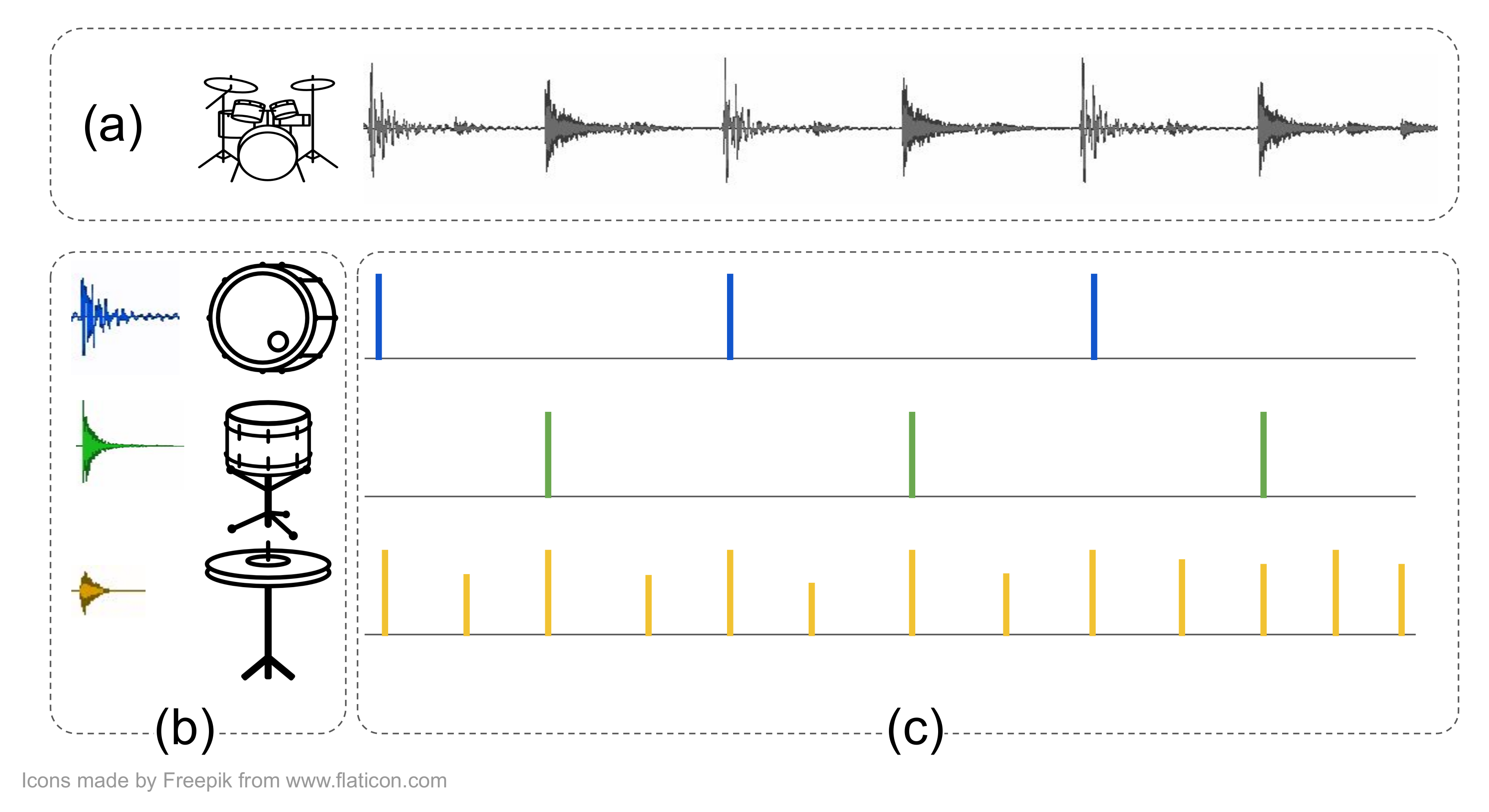
1.1. Drum Mixture Decomposition

In this paper, we consider the task of automatic unsupervised drum mixture decomposition, in which a percussive recording is decomposed into its constituent parts, while transcribing the onset locations of those instruments. A hypothetical example of such a decomposition is shown in Figure 1.

Such a decomposition enables applications such as, e.g., automatic music transcription, automatic drum sample extraction [1], or automatic redrumming [2].

The drum mixture decomposition problem described above is closely related to the problem of automatic drum transcription (ADT). ADT aims to detect and classify drum sounds events within a music recording, resulting in a list of onset locations for each transcribed instrument. Wu et al. [3] give a comprehensive overview of the state-of-the-art in ADT, and perform an in-depth comparison of these methods. They identify two classes of “activation-based” methods that currently dominate the state-of-the-art, namely, on the one hand neural network based systems using Recurrent Neural Network [4,5] or Convolutional Neural Network [6] architectures, and on the other hand methods based on non-negative matrix factorization (NMF) [3,7]. According to their analysis, neural network-based approaches outperform NMF-based methods in terms of transcription accuracy when a large and diverse training dataset with high-quality annotations is available. Such a dataset is not always available, however, and in the absence of such a dataset, NMF-based approaches offer a good alternative, as they do not require a data-hungry training procedure and still provide adequate performance if appropriately initialized. They are also more robust for drum mixtures with previously unseen instruments [3]. Unsupervised transcription systems, such as the ones based on NMF, can furthermore be used to improve supervised approaches by leveraging them in semi-supervised learning schemes such as student–teacher learning [8].

In this work, we build upon the non-negative matrix factor deconvolution (NMFD) algorithm, an extension of NMF that explicitly models sounds with a temporal structure [9]. We use NMFD not only to discover the onset locations within the mixture: at the same time, it discovers a “template” of the constituent sounds that are responsible for each set of onsets. We furthermore use NMFD in an unsupervised fashion, i.e., after a best-effort initialization with templates of common percussive sounds, we allow the model to freely optimize the discovered templates to the target mixture without imposing any constraints on the sonic characteristics of the instruments that we expect to find. This is in contrast with most of existing ADT work, where often a predefined and fixed set of percussive instruments is considered. Therefore, we use the term automatic drum mixture decomposition in order to distinguish this use case from ADT, which is concerned with discovering the onset locations of an often predefined and fixed set of percussive instruments. In the next section, we describe the NMFD algorithm and present an overview of related work using NMFD for drum mixture transcription and decomposition.

1.2. Non-Negative Matrix Factor Deconvolution for Drum Mixture Decomposition

The non-negative matrix factor deconvolution (NMFD) algorithm [9] can be used for the drum mixture decomposition problem introduced in Section 1.1. It decomposes a non-negative matrix $X\in {\mathbb{R}}_{\ge 0}^{N\times T}$ with N frequency bins and T time frames into a dictionary of K time-varying spectral templates $W^{\left(k\right)}\in {\mathbb{R}}_{\ge 0}^{N\times L}$, each L time frames long, and an activation matrix $H\in {\mathbb{R}}_{\ge 0}^{K\times T}$. The matrix X is modeled as the convolution of the templates with the activation matrix:

$$X_{n,t}\approx {\widehat{X}}_{n,t}=\sum _{k=1}^K\sum _{\tau =1}^L{W}_{n,\tau }^{\left(k\right)}{H}_{k,t-\tau },$$

(1)

where $H_{k,t-\tau }$ is zero when $t<\tau$. $W^{\left(k\right)}$ and H are updated iteratively using multiplicative updates in order to minimize a divergence measure $\mathcal{L}(X,\widehat{X})$, typically the least squares loss, Kullback–Leibler (KL) divergence or Itakura–Saito divergence [10]. There also exists a two-dimensional variant of NMFD [11].

The templates $W^{\left(k\right)}$ can be interpreted as short spectrograms of length L that model the constituent sounds of the mixture. The corresponding activation curves $H_k$, i.e., the rows of H, describe where in the recording these sounds occur. In order for this interpretation to make sense, each sound should repeat itself almost unaltered throughout the recording, so that the templates captured by $W^{\left(k\right)}$ can be “copied and pasted” at locations specified by $H_k$. This is a reasonable assumption for percussive instruments: hits on the same instrument will all sound approximately the same and will decay approximately equally fast, provided that the playing technique is consistent.

NMFD has already been applied successfully for automated drum transcription and drum separation tasks [1,10,12,13,14,15]. For example, Laroche et al. [13] use a combination of NMF and NMFD in order to perform harmonic-percussive sound separation, modeling the non-percussive sounds using NMF and the percussive sounds using NMFD with predefined and fixed templates $W^{\left(k\right)}$. The percussive template dictionary is constructed by hand prior to decomposition, and the separated harmonic and percussive audio are obtained by means of Wiener filtering [16]. Lindsay-Smith et al. [12] investigate the use of sparsity constraints on the activations H in order to obtain impulse-like onsets. Ueda et al. [14] rewrite NMFD for drum transcription within a Bayesian framework, and impose a constraint on the time-quantized score S, which is derived from the activations H.

The aforementioned works apply NMFD to discover the activations H, for the purpose of ADT or audio source separation. In other works, NMFD has also been applied to capture the constituent drum samples in a recording as faithfully as possible in W; this is typically done in a score-informed setting, wherein the exact onsets of each instrument (and consequently H) are assumed to be known. NMFD is used as such in Dittmar and Müller [15], where the extracted percussive sounds are subsequently used to validate a transient restoration technique that is applied when converting spectral representation back to an audible waveform. In Dittmar and Müller [1], the authors apply NMFD to estimate the drum sounds in the Amen Break, a well-known drum solo recording, in a score-informed setting. They observe that the unconstrained application of NMFD can lead to cross-talk artifacts, and they therefore propose two extensions to purify the extracted templates. Vande Veire et al. [17] apply NMFD in an uninformed setting, and they use an ad hoc modification of the update procedure for the templates $W^{\left(k\right)}$ in order to ensure that only a single drum hit is captured per template when using a long template length L.

While the cited works illustrate the effectiveness of NMFD for drum mixture transcription and (score-informed) decomposition, they also share the shortcoming that NMFD is usually applied in a constrained setting. When NMFD is applied for ADT, i.e., to discover the activations H, then the templates W are usually predefined and kept fixed during optimization. This limits the application to drum mixtures where a reasonably accurate approximation of the constituent drum sounds is known in advance. On the other hand, when NMFD is applied to discover the constituent sounds, i.e., the templates W, then this is done in a score-informed setting, where H is assumed to be known in advance. With the works in Ueda et al. [14] and Vande Veire et al. [17] as exceptions, we note the absence in the literature of a successful application of NMFD where both W and H are optimized jointly (Note that there are examples in the literature of the application of (regular) NMF for automatic drum transcription with a joint optimization of the (one-dimensional) templates W and the activations H [7,18]). Such a joint optimization could be useful, though, as it would allow to decompose a drum mixture for which neither the exact onsets H nor a sufficient approximation of W are available in advance.

In this paper, we therefore investigate the application of NMFD to jointly decompose a drum mixture into its templates W and their activations H. However, we note from previous work on NMFD for drum mixture decomposition [1,12,17] that applying NMFD unconstrainedly can lead to undesired artifacts or decompositions. Consequently, additional measures are required to guide the optimization to the desired, musically valid, and informative solution. In this work, we therefore enforce impulse-like behavior on the activations H, as detailed in Section 1.3.

1.3. Motivation for a Sigmoidal Model for the Activations

Percussive instruments are hit very briefly by some percussion mallet or beater; this implies that the discovered activations should be impulse-like, as the produced sounds results from an excitation that itself is an impulse. This is not enforced by the original NMFD model, however; consequently, when applied to drum mixtures, we observe that NMFD often does not lead to the expected impulse-like activations, as shown in Figure 2. This example illustrates that NMFD discovers activations with a sharp initial peak when a percussive hit occurs in the mixture, succeeded by a pseudo-exponentially decaying “tail’ of small activation values. There are also small activations throughout each activation curve that do not succeed a larger peak, which makes the decomposition hard to interpret: do these activations correspond to a detected drum hit, or not?

To address these shortcomings, additional constraints are needed to guide the decomposition process. One approach would be to enforce an L1 sparsity constraint on the activations H [12,19]. This encourages the algorithm to “move” as much information as possible from the activations H to the templates W, which would lead to sparser and potentially more impulse-like activations. This approach has a drawback, however, i.e., it also penalizes correct activations. This biases the model to capture sequences of successive drum strokes within a single template, in order to keep the activations as sparse as possible [12,17].

In this paper, we use an alternative approach in order to achieve the desired impulse-like behavior: we enforce that the activations take binary values, i.e., either an instrument is hit, which yields an activation value of 1, or an instrument is not hit, which yields an activation value of 0. The relation between this constraint and the desired impulse-like behavior becomes clear when considering that enforcing such binary activations rules out the aforementioned “tails” and unclear activations: either an instrument is hit, or it is not, and values in-between 0 (not hit) and 1 (hit) are discouraged. An advantage of this constraint is that it does not penalize legitimate peaks, as opposed to a sparsity constraint.

To achieve the proposed binary activations, we redefine the activations in the model as the logistic function of a logit-activations matrix, and we impose a regularization term that pushes the activations towards the saturating regions of the logistic curve during optimization. As such, non-binary activation values are discouraged, and the activation values will be pushed to either 0 or 1 as much as possible. Of course, different sources can be present in the mix at different volumes: this is modeled by multiplying the binary activations with a per-component amplitude factor. A log-power spectrogram representation is used, as this further reduces the impact of velocity differences and emphasizes the binary behavior of the onsets. Note that we choose to maintain a continuous transition between the two saturated states, instead of choosing for a fully discrete quantization of the activation values: this ensures that the model and objective function remain differentiable so that the optimization procedure is tractable, and additionally allows some flexibility in activation values. Through evaluation on a public dataset, we show that these adaptations lead to decompositions with the desired impulse-like activations, and we illustrate by means of an example that this can make the obtained unsupervised decompositions more interpretable.

1.4. Contributions

The main contributions of this paper are the following.

• We reformulate the activations in the NMFD model as the product of a per-component amplitude factor, representing the relative volume of each component, with the time-varying activations for each component.
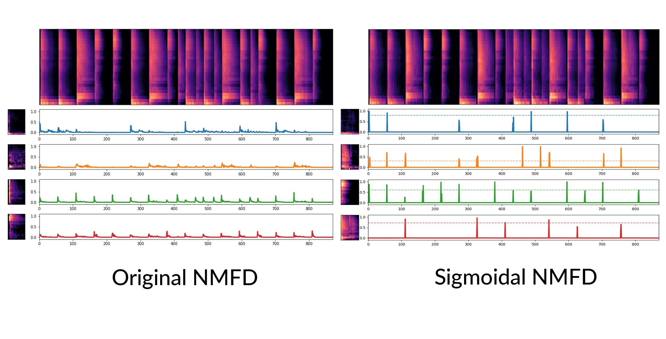
• These time-varying activations are defined as the output of a saturating sigmoidal function, and we propose a novel regularization term that combined with these saturating activations leads to binary activations. We show that in the context of automatic drum mixture decomposition, the activations are not only binary, but also become impulse-like as a consequence of this method.
• We propose different strategies and techniques to optimize the proposed model, and we rigorously evaluate their efficacy in minimizing the overall objective function for the decomposition.
• We propose metrics to evaluate the unsupervised decomposition of drum mixtures. With these, we show that the proposed algorithm achieves more impulse-like activations compared to unconstrained NMFD and sparse NMFD, making it better suited to the properties of percussive mixtures, while yielding a good decomposition and spectrogram reconstruction quality.

1.5. Structure of This Paper

The remainder of this paper is structured as follows. Section 2 introduces the modified NMFD algorithm and the procedure that is used to optimize this model. Section 3 describes the baseline models, dataset, metrics, and experimental details. Section 4 discusses the experimental results, and Section 5 concludes the paper and outlines directions for further research.

2. NMFD with Saturating Activations

2.1. Sigmoidal NMFD Model

The logistic function $\sigma (·)$ is defined as

$$\sigma \left(x\right)=\frac{1}{1+exp(-x)}.$$

(2)

For large positive values of the input, $\sigma \left(x\right)$ saturates to 1, and for large negative values of the input, it saturates to 0. If $y=\sigma \left(x\right)$, then x is also called the logit of y.

We rewrite the NMFD model using saturating activations:

$$X_{n,t}\approx {\widehat{X}}_{n,t}=\sum _{k=1}^K\sum _{\tau =1}^L{W}_{n,\tau }^{\left(k\right)}\sigma \left(a_k\right)\sigma \left(G_{k,t-\tau }\right),$$

(3)

with $X\in {\mathbb{R}}_{\ge 0}^{N\times T}$, $W^{\left(k\right)}\in {\mathbb{R}}_{\ge 0}^{N\times L}$, $G\in {\mathbb{R}}^{K\times T}$ and $a\in {\mathbb{R}}^K$. X and $W^{\left(k\right)}$ are scaled to maximum amplitude 1. By comparing Equations (1) and (3), we see that for the sigmoidal model, $H_{k,t}=\sigma \left(a_k\right)\sigma \left(G_{k,t}\right)$. The sigmoidal activations $\sigma \left(G_{k,t}\right)$ capture the onsets for each component k, while the amplitudes $\sigma \left(a_k\right)$ capture the relative volume of each component, as different components $W^{\left(k\right)}$ and $W^{\left(l\right)}$ can be present at different volumes in the mix. Note that the logit-activations $G_{k,t}$ and the logit-amplitudes $a_k$ can take negative values.

2.2. Objective Function

The main objective of the decomposition is to minimize the divergence between the input spectrogram and the approximation. In this paper, we use the KL divergence:

$${\mathcal{L}}_{\mathrm{KL}}(X,\widehat{X})=\sum _{n,t}{X}_{n,t}ln\left(\frac{X_{n,t}}{{\widehat{X}}_{n,t}}\right)-X_{n,t}+{\widehat{X}}_{n,t}.$$

(4)

We furthermore want the activations to be binary in nature: for each t, the template $W^{\left(k\right)}$ should either be fully active, $\sigma \left(G_{k,t}\right)\approx 1$, or not active at all, $\sigma \left(G_{k,t}\right)\approx 0$ (Note that the logistic function $\sigma \left(x\right)$ is never exactly equal to either 0 or 1 for real values of the logit x; this is only the case in the limit for $x\to -\infty$ and for $x\to +\infty$, respectively. Therefore, it would be more correct to say that the activations take approximately binary values.). In other words, $\sigma \left(G_{k,t}\right)$ must be in a saturating region of $\sigma$ for all k and t. To achieve this, we define an additional regularization term ${\mathcal{L}}_G$:

$$\begin{array}{c}{\mathcal{L}}_G\left(G\right)=\sum _{k,t}exp\left\{-{\left(\frac{G_{k,t}-{\mu }_k}{2}\right)}^2\right\},\end{array}$$

(5)

$$\begin{array}{c}{\mu }_k={\sigma }^{-1}\left({\alpha }_k\underset{t}{max}\left(\sigma \left(G_{k,t}\right)\right)+(1-{\alpha }_k)\underset{t}{min}\left(\sigma \left(G_{k,t}\right)\right)\right).\end{array}$$

(6)

Here, ${\sigma }^{-1}$ is the inverse of the logistic function, and ${\alpha }_k=0.5$. This regularization term encourages all logit activations $G_{k,t}$ of the $k^{\mathrm{th}}$ component to lie as far away as possible from the logit ${\mu }_k$ of the center activation value $\sigma \left({\mu }_k\right)$, and ${\mathcal{L}}_G\left(G\right)$ is minimal when all activations saturate to either 0 or 1.

The sigmoidal NMFD model, Equation (3), thus optimizes the following objective function:

$${\mathcal{L}}_{\mathrm{tot}}(X,\widehat{X},G)={\mathcal{L}}_{\mathrm{KL}}(X,\widehat{X})+\gamma {\mathcal{L}}_G\left(G\right).$$

(7)

The hyperparameter $\gamma$ weighs the relative importance of the regularization term ${\mathcal{L}}_G$ with respect to the spectrogram reconstruction objective ${\mathcal{L}}_{\mathrm{KL}}$; in this paper, we set $\gamma =1$.

2.3. Optimization Procedure

2.3.1. Optimization Procedure Overview

Like the original NMFD algorithm [9], the model parameters $W_{n,\tau }^{\left(k\right)}$, $G_{k,t}$ and $a_k$ are optimized in order to obtain a minimal loss ${\mathcal{L}}_{\mathrm{tot}}$ by means of an iterative optimization procedure. First, the parameters are initialized as explained in Section 3.2. Then, G, W and a are updated iteratively as follows:

• Calculate $\widehat{X}$ using the most recent estimates for W, G and a, as in Equation (3);
• Update the logit-activations G, see Section 2.3.2, Equation (9);
• Calculate $\widehat{X}$ again with the new estimate for G;
• Update the templates $W^{\left(k\right)}$, see Section 2.3.3, Equation (12);
• Calculate $\widehat{X}$ again with the new estimate for W;
• Update the component-wise amplitudes a, see Section 2.3.4, Equation (13);
• Repeat these steps until convergence.

2.3.2. Additive Gradient-Descent Update for G

${\mathcal{L}}_{\mathrm{tot}}$ is minimized with respect to G using gradient-descent:

$$\begin{array}{cc}\hfill G_{k,t}& \leftarrow G_{k,t}-{\eta }_G\frac{\partial {\mathcal{L}}_{\mathrm{tot}}(X,\widehat{X},G)}{\partial G_{k,t}}\hfill \end{array}$$

(8)

$$\begin{array}{cc}\hfill & =G_{k,t}-{\eta }_G\left(\frac{\partial {\mathcal{L}}_{\mathrm{KL}}}{\partial G_{k,t}}+\gamma \frac{\partial {\mathcal{L}}_G}{\partial G_{k,t}}\right).\hfill \end{array}$$

(9)

The learning rate ${\eta }_G$ is a hyperparameter of the optimization procedure. The partial derivatives in Equation (9) expand to (see Appendix A.1):

$$\begin{array}{cc}\hfill \frac{\partial {\mathcal{L}}_{\mathrm{KL}}}{\partial G_{k,t}}& =\sum _{n,\tau }\left(1-\frac{X_{n,t+\tau }}{{\widehat{X}}_{n,t+\tau }}\right)\sigma \left(G_{k,t}\right)\sigma (-G_{k,t})W_{n,\tau }^{\left(k\right)}\sigma \left(a_k\right),\hfill \end{array}$$

(10)

$$\begin{array}{cc}\hfill \frac{\partial {\mathcal{L}}_G}{\partial G_{k,t}}& \approx -\left(G_{k,t}-{\mu }_k\right)exp\left\{-{\left(\frac{G_{k,t}-{\mu }_k}{2}\right)}^2\right\}.\hfill \end{array}$$

(11)

Note that we regard ${\mu }_k$ as a constant in the derivation of Equation (11). The expression for $\frac{\partial {\mathcal{L}}_G}{\partial G_{k,t}}$ is thus only approximately correct when $G_{k,t}={max}_{t^{\prime }}\left(G_{k,t^{\prime }}\right)$ or $G_{k,t}={min}_{t^{\prime }}\left(G_{k,t^{\prime }}\right)$. We do so in order to avoid instabilities in the updates for the ultimate values of the activations, see Appendix A.1 for details.

2.3.3. Multiplicative Update for W

W is optimized using a multiplicative update rule, which ensures that W remains strictly positive. Its derivation from Equation (7) is analogous to that in Schmidt and Mørup [11], see Appendix A.2. This gives

$$W_{n,\tau }^{\left(k\right)}\leftarrow W_{n,\tau }^{\left(k\right)}\frac{{\sum }_t\sigma \left(a_k\right)\sigma \left(G_{k,t-\tau }\right)\left(\frac{X_{n,t}}{{\widehat{X}}_{n,t}}\right)}{{\sum }_t\sigma \left(a_k\right)\sigma \left(G_{k,t-\tau }\right)}.$$

(12)

After each update, $W^{\left(k\right)}$ is scaled to maximum amplitude 1 for each k.

2.3.4. Additive Gradient-Descent Update for a

${\mathcal{L}}_{\mathrm{tot}}$ is minimized with respect to a using gradient-descent:

$$a_k\leftarrow a_k-{\eta }_a\frac{\partial {\mathcal{L}}_{\mathrm{tot}}(X,\widehat{X},G)}{\partial a_k},$$

(13)

where ${\eta }_a$ is the learning rate and with $\frac{\partial {\mathcal{L}}_{\mathrm{tot}}}{\partial a_k}$ given by (see Appendix A.3)

$$\begin{array}{cc}\hfill \frac{\partial {\mathcal{L}}_{\mathrm{tot}}}{\partial a_k}& =\sigma \left(-a_k\right)\sum _{n,t}\left[\left(1-\frac{X_{n,t}}{{\widehat{X}}_{n,t}}\right)\sum _{\tau }{W}_{n,\tau }^{\left(k\right)}\sigma \left(a_k\right)\sigma \left(G_{k,t-\tau }\right)\right].\hfill \end{array}$$

(14)

2.3.5. Optimization Strategies to Escape Local Minima

The model parameters are updated by iteratively applying Equations (9), (12), and (13). This is, however, a delicate task, as it is prone to converge to poor local minima due to the regularization term ${\mathcal{L}}_G$. In the update for G, this regularization namely pushes $G_{k,t}$ away from ${\mu }_k$, see Equation (11). If the algorithm has not converged yet, then this prevents new peaks to grow or existing peaks to shrink, even if this would eventually lead to a better optimum. Imposing ${\mathcal{L}}_G$ too strongly or too early during optimization could therefore hinder convergence to a better local minimum.

We therefore propose and evaluate three optimization strategies that could help to find better local minima, as detailed below. In general, the optimization happens in different stages: an unconstrained warm-up stage, an explore-and-converge stage, and an ultimate finalization stage.

The goal of the unconstrained warm-up stage is to make the algorithm converge from its initialization (see Section 3.2) to a rough approximation of the spectrogram and a first estimation of the activation functions. During this stage, $\gamma =0$, so that in this initial exploration, the activations are free to converge to the values that best approximate the spectrogram. We furthermore set ${\eta }_G=0.5$, and ${\eta }_a$ is set to $0.02$. The warm-up stage is 30 iterations long. Empirically, this leads to good results in our experiments.

After the warm-up stage comes the explore-and-converge stage, wherein the proposed saturation regularization is applied and where an optimal solution is sought for the decomposition problem. In this paper, we consider the following strategies to execute this stage:

• Optimization strategy 0: straightforward optimization.
  In this strategy, ${\mathcal{L}}_G$ is applied with $\gamma =1.0$ at each iteration, and ${\mu }_k$ is calculated as in Equation (6) with ${\alpha }_k=0.5$.
• Optimization strategy 1: staged application of ${\mathcal{L}}_G$.
  In this strategy, we periodically enable and disable ${\mathcal{L}}_G$ by alternating between “saturation sub-stages” and “fine-tuning sub-stages”, which each last several iterations. During a saturation sub-stage, $\gamma =1$, so that the activations are pushed towards saturation. During a fine-tuning sub-stage, $\gamma =0$, so that the model has time to make peaks grow or shrink against the direction imposed by ${\mathcal{L}}_G$, in order to escape poor local minima.
• Optimization strategy 2: moving ${\mu }_k$ throughout optimization.
  In this strategy, we impose ${\mathcal{L}}_G$ at each iteration, i.e., $\gamma =1.0$ for each update. In order to avoid squashing small peaks too early and additionally provide an incentive to escape local minima, we move around the “center point”${\mu }_k$ of ${\mathcal{L}}_G$ (Equation (6)) by changing ${\alpha }_k$ in each iteration. More specifically, for each update of G and component k, we set ${\alpha }_k$ to a random value drawn from a uniform distribution over the interval $(0.05,0.25)$. We hypothesize that setting ${\alpha }_k$ to a relatively low value (${\alpha }_k<0.5$) helps to boost relatively small peaks, and that randomly sampling ${\alpha }_k$ could help to escape local optima.
• Optimization strategy 3: combine strategy 2 and strategy 3.
  This strategy combines the two aforementioned strategies: ${\mathcal{L}}_G$ is enabled and disabled alternatingly, and when it is applied, ${\mu }_k$ is moved around by sampling ${\alpha }_k$ from a uniform distribution over $(0.05,0.25)$ for each update of G.

During the explore-and-converge stage, we set ${\eta }_G=0.2$, as we find that this leads to a good convergence in our experiments. The learning rate ${\eta }_a$ for the amplitudes a remains unchanged, i.e., ${\eta }_a=0.02$. We perform 180 iterations in total during this stage. For strategy 1 and strategy 3, each sub-stage is 30 iterations long, so that the explore-and-converge stage consists of three repetitions of alternating saturation and fine-tuning sub-stages.

The finalization stage concludes the optimization process. It consists of a final 30 iterations, in which we set $\gamma =1$, ${\eta }_G=0.1$, ${\eta }_a=0.02$, and ${\alpha }_k=0.5$. This allows the algorithm to converge to the final solution.

In our experiments, we found that normalizing the gradients of G and a in Equations (9) and (13) to a maximum amplitude of 1 for each component is important to ensure that the activations in each activation curve $G_k$ grow equally quickly. Otherwise, one component could grow much quicker than the others and start to dominate the decomposition, often resulting in a poor local optimum of ${\mathcal{L}}_{\mathrm{tot}}$ where only one component is active (also see Section 4.2).

3. Experimental Set-Up

3.1. Baseline Models

We consider two baseline models to compare with. The first baseline model uses the original NMFD formulation from Equation (1) without additional constraints. The second baseline adds an L1 sparsity constraint with weighing factor $\lambda$ to the objective function, Equation (4):

$$\begin{array}{cc}\hfill \mathcal{L}(X,\widehat{X},H)& ={\mathcal{L}}_{\mathrm{KL}}(X,\widehat{X})+\lambda {\mathcal{L}}_{\mathrm{L}1}\left(H\right)\hfill \end{array}$$

(15)

$$\begin{array}{cc}\hfill & ={\mathcal{L}}_{\mathrm{KL}}(X,\widehat{X})+\lambda \sum _{k,t}\left|H_{k,t}\right|.\hfill \end{array}$$

(16)

In our experiments, we consider sparsity weights of $\lambda =1.0$ (strong sparsity constraint), $\lambda =0.1$ (medium sparsity constraint), and $\lambda =0.01$ (weak sparsity constraint).

For both the unconstrained NMFD baseline and the L1-constrained baselines, we use the update rules from Schmidt and Mørup [11], as we observed numerical instabilities for the original NMFD update rules from the work in Smaragdis [9] when $W^{\left(k\right)}$ contains columns that are much smaller in amplitude than other columns, i.e., when the sample captured by $W^{\left(k\right)}$ is silent at certain points. Similar observations were made in Lindsay-Smith et al. [12]. As for the sigmoidal model, 240 update iterations are performed. We furthermore evaluate two optimization strategies for the sparse baselines. In the first, L1 regularization is applied throughout the entire optimization, starting from the first iteration. In the second, the L1 regularization is disabled for the first 30 iterations, i.e., $\lambda$ is set to 0. The reason for this second optimization strategy is that applying the L1 regularization too early might hinder proper convergence. This allows to evaluate whether the baselines would benefit from an “unconstrained warm-up stage” as used for the sigmoidal model.

For all baselines, the spectral templates $W^{\left(k\right)}$ are initialized in the same way as for the sigmoidal model, see Section 3.2, and are scaled to max amplitude 1 after each update as in the sigmoidal model. The activations H are initialized with random values drawn from a uniform distribution over $(0,{10}^{-3})$.

3.2. Model Initialization

L is set to 50, which at a sample rate of 44,100 Hz and short-time Fourier transform (STFT) hop size of 256 corresponds to a template length of 290 ms. We set the number of components K to the number of percussive instruments in the mixture, which we assume is known in advance.

The templates $W^{\left(k\right)}$ are initialized using an averaged spectrogram template of drum hits of four common drum instruments: kick drum, snare drum, hi-hat, and crash cymbal. These average templates are created using a small dataset of individual drum hits [20], by averaging the aligned spectra of the single-hit samples of the desired instrument type. The first four components are initialized with a kick, hi-hat, snare, and crash template; if $K>4$, then the excess components are initialized by alternating between the hi-hat template and the snare drum template. Each $W^{\left(k\right)}$ is also rescaled to a maximum amplitude of 1.

For the sigmoidal model, the logit-activations $G_{k,t}$ are initialized with random values drawn from a uniform distribution over the interval $\left(-5,-4\right)$ so that $\sigma \left(G_{k,t}\right)\in \left(0.0067,0.018\right)$. The logit-amplitudes $a_k$ are initialized to 2, so that $\sigma \left(a_k\right)\approx 0.9$.

3.3. Dataset

The algorithm is evaluated on the ENST dataset [21], which contains annotated recordings of percussion-only pieces performed by three drummers on three different drum kits using a variety of beaters (sticks, rods, mallets, and brushes). We only use the wet mix of the “phrase” recordings, i.e., short drum sequences in various popular styles. There are 135 phrases in total, varying in tempo (labeled “slow”, “medium”, and “fast” in the dataset), and complexity (“simple”, i.e., straight and without ornaments, and “complex”, i.e., with fill-ins and ornaments). We modify the recordings slightly by cutting away the last hit of each recording. The motivation for this is that the last hit often “rings out”, i.e., it has a long decay, which cannot be appropriately modeled in the NMFD paradigm, given the fixed and limited template length L (Note that, while hits on the same component as the last hit should have the same decay time, we do not observe any issues with modeling these hits throughout the mixture. We note two reasons for this. First, when an instrument with a long decay is hit, it is typically hit again before the first hit can fully “ring out”, i.e., its decay is “cut short” by the second hit. Second, the low-volume “tail” of the decay is often masked by the sound of subsequent hits on other components. These two effects effectively reduce the template length L that is required to model the sounds in the mixture, except for the last hit where these effects do not apply. An alternative solution would be to increase L in order to fully capture these hits with a long decay within a single template. We choose not to do so, however, as this makes the optimization of the NMFD algorithm hard and prone to error, as discussed in Vande Veire et al. [17].).

3.4. Spectrogram Representation

For the experiments in this paper, we use a custom Mel-frequency-scale log-power spectrogram representation. This spectral representation is designed to reduce computation time to obtain the decomposition, while maintaining a sufficiently fine resolution in order to distinguish all relevant sounds in the mixture.

The audio sample rate is 44,100 Hz. First, the STFT power spectrogram $X={\left|STFT\left(y\right)\right|}^2$ of the audio y is calculated using a frame length of 2048, a hop size of 256, and a Hann window over the frames. Then, the values of the STFT spectrogram are rescaled to the range $(0,1)$, and they are summed along the frequency axis over N adjacent, non-overlapping frequency bands. The boundary frequencies of these bands are spaced according to a Mel-scale between 0 Hz and 11,025 Hz. Finally, a small value ${ϵ}_{\mathrm{pre}-\mathrm{dB}}$ is added to the power spectrogram, which is then converted to a decibel scale and scaled to the range $({ϵ}_{\mathrm{post}-\mathrm{dB}},1)$.

Using the Mel scale makes the low to mid frequencies much more prominent in the resulting spectrogram as compared to a linear scale spectrogram, where a higher proportion of the bins would be allocated for higher frequencies. Using non-overlapping windows ensures that each STFT bin only contributes to one Mel-scale bin, so that the resulting spectrogram is less blurred. We find that these properties help to better distinguish between different instruments, especially those with a prominent presence in the low and mid frequencies (kick drum, snare drum, toms, bongos, etc.). A small number of bins N significantly reduces the time needed to decompose the spectrogram. We find that a limited number of bins is sufficient for a good decomposition and choose $N=25$. Adding a small value ${ϵ}_{\mathrm{pre}-\mathrm{dB}}$ before the decibel transformation masks low-valued noise, so that the resulting dB-scale spectrogram optimally uses its value range to differentiate between relevant power differences, making it clearer and easier to decompose. Scaling the spectrogram values to values in $({ϵ}_{\mathrm{post}-\mathrm{dB}},1)$ after transforming it to a dB scale is required for the sigmoidal model to be able to approximate all spectrogram values, while a minimum value of ${ϵ}_{\mathrm{post}-\mathrm{dB}}$ is used to avoid numerical instabilities in various computations. We set ${ϵ}_{\mathrm{pre}-\mathrm{dB}}={10}^{-7}$ and ${ϵ}_{\mathrm{post}-\mathrm{dB}}={10}^{-9}$.

3.5. Evaluation Metrics

In our evaluation, we wish to quantify the quality of unsupervised decompositions of drum mixtures, and compare these quantities for the outcome of the sigmoidal model and of the baseline models. Note that the unsupervised nature of the decomposition makes it more difficult to rely on ground-truth transcriptions of the music, as due to the unsupervised character there is no guarantee that the extracted components would match one-to-one with instruments in the music. Turning NMFD into a transcription algorithm would require incorporating some supervision mechanism that guides the components $W^{\left(k\right)}$ to the desired musical interpretation, which is beyond the scope of this paper. Therefore, alternative evaluation metrics need to be used that quantify the quality or “usefulness” of such unsupervised decompositions.

We consider a decomposition to be of a good quality if

• the spectrogram is approximated well;
• all onsets in the mixture are detected, with as few false onset detections as possible;
• different components have different activation patterns: this means they contribute to the spectrogram at different times, which might indicate a more meaningful differentiation between components; and
• the activations are impulse-like.

The metrics to quantitatively assess these criteria are described in the following subsections. Some metrics are calculated over the activations $H_{k,t}$; when evaluated for the sigmoidal model, $H_{k,t}$ should be substituted by $\sigma \left(G_{k,t}\right)$ in these metrics.

3.5.1. Spectrogram Reconstruction Quality

The spectrogram reconstruction quality is measured using the mean absolute error (MAE) between the target spectrogram and its reconstruction:

$$MAE(X,\widehat{X})=\frac{1}{NT}\sum _{n,t}\left|X_{n,t}-{\widehat{X}}_{n,t}\right|.$$

(17)

As all spectrogram values are scaled between $({ϵ}_{\mathrm{post}-\mathrm{dB}},1)$, MAE values of different spectrograms can be compared.

3.5.2. Overall Onset Coverage

We measure whether each onset in the drum mixture is accounted for by the decomposition, although without considering instrument information. First, peak picking is performed on each row of H. A value $H_{k,t}$ at an offset t is considered to be a peak if it satisfies three conditions [22]:

• $H_{k,t}=max\left(H_{k,t-{\tau }_{\max }:t+{\tau }_{\max }}\right)$,
• $H_{k,t}\ge \mathrm{mean}\left(H_{k,t-{\tau }_{\mathrm{avg}}:t+{\tau }_{\mathrm{avg}}}\right)+{\theta }_{\mathrm{thr}}{max}_t\left(H_{k,t}\right)$,
• $t-t_{\mathrm{prev}}>{\tau }_{\mathrm{wait}}$,

where $t_{\mathrm{prev}}$ is the offset of the last peak detected before t and where the hyperparameters are set as ${\tau }_{\max }=5$ (corresponding to 29 ms), ${\tau }_{\mathrm{avg}}={\tau }_{\mathrm{wait}}=10$ (58 ms). We vary the value of the peak picking threshold ${\theta }_{\mathrm{thr}}$ within the range of $(0.1,0.9)$ in order to evaluate its influence on the metric proposed below.

The detected peaks are then shifted by the “template offset” ${\tau }_{\mathrm{off}}^{\left(k\right)}$, which is calculated as the smallest value of $\tau$ for which the envelope of $W^{\left(k\right)}$, $w^{\left(k\right)}\left[\tau \right]={\sum }_n{W}_{n,\tau }^{\left(k\right)}$, is larger than the average envelope value: ${\tau }_{\mathrm{off}}^{\left(k\right)}=min\left(\{\tau :w^{\left(k\right)}\left[\tau \right]\ge \frac{1}{L}{\sum }_{\tau }{w}^{\left(k\right)}\left[\tau \right]\}\right)$. This is necessary as the percussive hit modeled by $W^{\left(k\right)}$ might be shifted by some offset ${\tau }_{\mathrm{off}}^{\left(k\right)}$ in the template.

These peaks are then compared with the ground-truth annotations. A peak in the decomposition is considered a true positive if there is a ground-truth onset of any instrument within the tolerance interval of 29 ms around that peak; otherwise, it is a false positive. Ground-truth annotations for which there is no peak detected within the tolerance interval around it are false negatives. The precision, recall, and F-measure are calculated using these true positive, false positive, and false negative counts.

Note that this metric allows a ground-truth onset to be “covered” by multiple activation peaks and vice versa, and that peaks from any component can match with onsets from any instrument. We do not attempt to match components with specific instruments in the ground-truth annotations, as this is a difficult task that is prone to error and ambiguity, and we consider this beyond the scope of the unsupervised decomposition that is considered in this paper.

3.5.3. Activation Curve Similarity

This metric quantifies how different the activations from each component are from the activations of any other component in the decomposition. We consider a decomposition to be of higher quality if the different activation curves are disentangled, i.e., they activate often at distinct times in the mixture. Each component then models drum hits that are not modeled by other components. On the other hand, a high similarity between activation curves indicates that multiple components often contribute to the same onsets, so that it could be difficult to figure out the relationship between instruments in the mixture and components in the decomposition.

Note that we expect the activations in the decomposition to have at least a low amount of similarity, as the onsets in different rhythmic instruments are often correlated and will coincide at least sometimes. However, an exceedingly high similarity value would be unexpected, as we expect distinct instruments to have at least some degree of uniqueness to their activations, and it is this undesired behavior that we wish to detect by using this metric.

To quantify activation curve similarity for a given activation matrix H, each activation curve is first smoothed and made non-zero using a running mean operation:

$${\overline{H}}_{k,t}=\frac{1}{2M+1}\sum _{u=-M}^M{H}_{k,t+u}+{ϵ}_H.$$

(18)

We set M to 5, corresponding to a symmetric tolerance interval of 29 ms around each t. This smoothing allows to better compare two activation curves that capture the same onsets but that are slightly shifted with respect to each other. Then, the cosine similarity is calculated between every pair of rows in H. The small value ${ϵ}_H={10}^{-52}$ ensures that comparing one row of H with an all-zero row in H still results in a meaningful metric value, for example, comparing two all-zero rows in H should result in a similarity value of 1. After calculating the pairwise similarity of all rows in H, we consider the minimum, mean and maximum similarity between any pair of rows to quantify the amount of differentiation between the activations for each decomposition.

A high value for the maximum similarity indicates that there are at least some components that detect more or less the same hits in the mixture, which is undesirable.

3.5.4. Peakedness Measure

This metric quantifies to what extent a decomposition is impulse-like, by comparing the original activation curve with a processed version in which peaks are accentuated and small values are removed. We define the half wave rectification operation $\mathrm{HWR}\left(x\right)\left[t\right]$ as

$$\mathrm{HWR}\left(x\right)\left[t\right]=max(x\left[t\right]-\overline{x}\left[t\right],0),$$

(19)

in which $\overline{x}$ is the smoothed version of x, see Equation (18). We furthermore define the compansion (compression-expansion) operation ${\mathrm{comp}}_{\kappa }\left(x\right)\left[t\right]$ with exponent $\kappa$ as

$${\mathrm{comp}}_{\kappa }\left(x\right)\left[t\right]=\underset{u}{max}\left(x\left[u\right]\right){\left(\frac{x\left[t\right]}{{max}_u\left(x\left[u\right]\right)}\right)}^{\kappa }.$$

(20)

If $\kappa >1$, then ${\mathrm{comp}}_{\kappa }\left(x\right)$ makes relatively small values even smaller compared to the maximum value of x, accentuating large values. If $\kappa <1$, then ${\mathrm{comp}}_{\kappa }\left(x\right)$ makes relatively small values larger. We then calculate the peak-accentuated version of $H_k$ as

$$H_{k,t}^{\mathrm{peaks}}={\mathrm{comp}}_{{\kappa }^{-1}}\left(\mathrm{HWR}\left({\mathrm{comp}}_{\kappa }\left(H_k\right)\right)\right)\left[t\right],$$

(21)

with $\kappa =3$. This operation should be understood as follows. First, the inner compansion accentuates the highest peaks in $H_k$, while making smaller peaks even smaller. The HWR operation then removes values that are smaller than the running mean around it, which further accentuates peaks and removes low-valued noise. The outer compansion then restores the peaks to their original relative scale, as long as they were not removed by the HWR operation.

The peakedness of an activation curve $H_{k,t}$ is defined as the ratio ${\sum }_t{H}_{k,t}^{\left(\mathrm{peaks}\right)}/{\sum }_t{H}_{k,t}$. If the ratio of the sum of values of $H_{k,t}^{\left(\mathrm{peaks}\right)}$ and $H_{k,t}$ is close to 1, then $H_{k,t}$ changed very little by the impulse-accentuating operation, i.e., it was already quite impulse-like itself. If the ratio is lower, however, then around the peaks in $H_{k,t}$ there must be low values that are removed by the HWR operation when calculating $H_{k,t}^{\left(\mathrm{peaks}\right)}$, meaning that the activations are less impulse-like.

We report the average of the peakedness values of all activation curves of H.

3.6. Implementation Details

Our NMFD implementation is loosely based on the NMFD implementation from López-Serrano et al. [23]. All code for this paper is made available on a public online repository [24].

4. Results

This section presents the evaluation of our method. Section 4.1 and Section 4.2 present the evaluation on the ENST dataset. Section 4.3 presents a case study to visually illustrate the effects of our method.

The purpose of our evaluation is twofold. The first objective is to compare the performance of the sigmoidal model and of the baselines in terms of the proposed evaluation metrics. This comparison is presented in Section 4.1 and

Table 1. Comparison of the performance of the NMFD baseline, the sparse NMFD baselines, and the proposed sigmoidal NMFD model on the evaluation metrics. For each metric, the mean value over all 135 phrases is shown (standard deviation between parentheses). The results for the peakedness metric for the strong sparsity baseline (*) are computed after discarding any all-zero activation curves in H. For each metric, the most optimal value is shown in bold in each column.

Algorithm	MAE	Overall Onset Coverage				Activations Similarity			Peakedness
		Pr.	Rec.	F-Score	F-Score (${\mathit{\theta }}_{\mathbf{thr}}=0.5$)	Min	Mean	Max	Mean
Unconstrained NMFD	0.025 (0.003)	0.76 (0.15)	0.94 (0.09)	0.83 (0.12)	0.63 (0.17)	0.45 (0.12)	0.63 (0.10)	0.79 (0.12)	0.42 (0.02)
NMFD + L1 sparsity          ($\lambda =0.01$)	0.026 (0.003)	0.77 (0.15)	0.94 (0.09)	0.84 (0.12)	0.61 (0.18)	0.39 (0.13)	0.59 (0.10)	0.77 (0.12)	0.43 (0.02)
NMFD + L1 sparsity          ($\lambda =0.1$)	0.037 (0.005)	0.76 (0.16)	0.91 (0.09)	0.82 (0.12)	0.50 (0.18)	0.04 (0.10)	0.19 (0.10)	0.65 (0.21)	0.45 (0.08)
NMFD + L1 sparsity          ($\lambda =1.0$)	0.071 (0.009)	0.88 (0.15)	0.84 (0.13)	0.85 (0.13)	0.35 (0.17)	0.15 (0.31)	0.57 (0.25)	0.90 (0.26)	0.46 * (0.13)
Sigmoidal NMFD (strategy 0, $\gamma =1.0$,       constant ${\eta }_G$)	0.044 (0.006)	0.83 (0.17)	0.78 (0.13)	0.79 (0.13)	0.70 (0.15)	0.07 (0.12)	0.23 (0.10)	0.51 (0.14)	0.72 (0.06)
Sigmoidal NMFD (strategy 2, $\gamma =0.1$)	0.035 (0.004)	0.79 (0.19)	0.88 (0.11)	0.82 (0.14)	0.73 (0.13)	0.12 (0.11)	0.28 (0.10)	0.56 (0.15)	0.67 (0.06)

. In this evaluation, the sigmoidal NMFD model is optimized with a simplified and straightforward optimization strategy, i.e., optimization strategy 0 with a constant learning rate ${\eta }_G$. Comparing with this simplified algorithm helps us understand to what extent the observed improvements are caused by the proposed model itself, rather than by certain elements in the optimization strategy (also see Section 4.2). For completeness, Table 1 also reports the results for the sigmoidal model optimized with the best performing optimization strategy, i.e., strategy 2 with $\gamma$ set to $0.1$ during the explore-and-converge stage.

The second objective of the evaluation is to provide an in-depth analysis of the additional gains that can be achieved by using more advanced optimization strategies. This analysis is provided in Section 4.2. We furthermore perform an ablation study to quantify the impact of several techniques we use in the optimization of our model. From this evaluation, we conclude that more advanced optimization strategies and techniques help to achieve better local minima of the objective function ${\mathcal{L}}_{\mathrm{tot}}$.

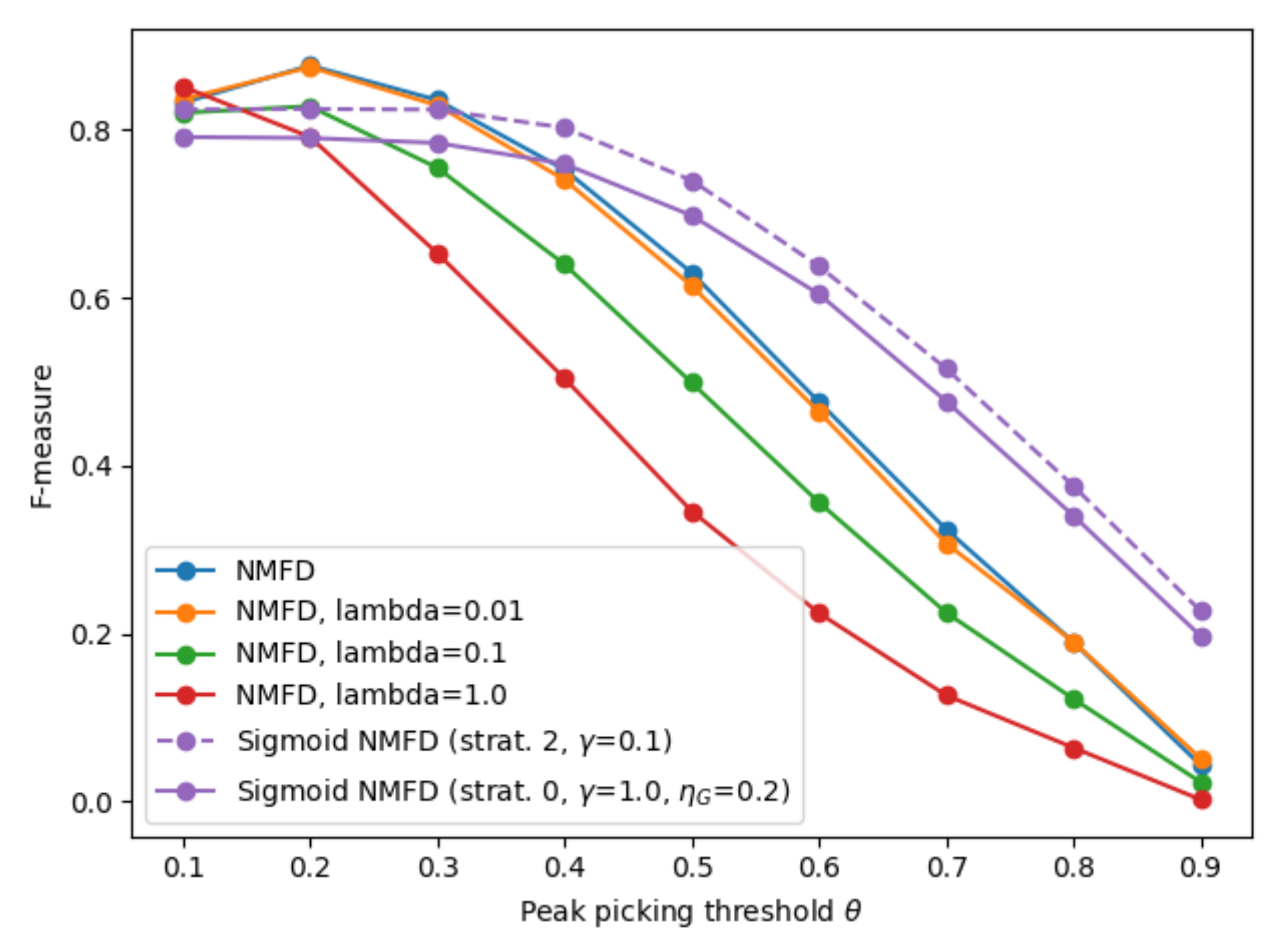
4.1. Evaluation on the ENST dataset

Table 1 shows the results of the evaluation on the ENST dataset.

As discussed in Section 3.1, the baselines are evaluated once with and once without an “unconstrained warm-up stage”. We found that performing a warm-up stage for optimizing the sparse baselines leads to virtually the same results as not using that technique, i.e., the outcome in terms of the metrics reported in Table 1 is exactly or almost exactly the same. For the sake of conciseness and not cluttering the Table, we therefore omit the results for the sparse baselines with a warm-up stage from Table 1. We conclude that the sparse baselines are not hindered in their convergence by applying regularization from the beginning of the optimization. The conclusions drawn in the following evaluation are therefore valid for all sparse baselines, regardless of whether or not an unconstrained warm-up stage has been applied.

Regarding the spectrogram reconstruction quality, the average MAE is low for most models, i.e., all spectrograms are approximated well. For the high sparsity baseline, the mean MAE is approximately twice as high as for the other models, suggesting that the L1 regularization in this baseline is too strong and leads to a worse spectrogram approximation. On average, the approximations by the medium sparsity baseline are comparable to those by the sigmoidal model in terms of MAE, and slightly worse than the unconstrained NMFD algorithm. This result is expected, as the unconstrained model optimizes only the reconstruction loss ${\mathcal{L}}_{\mathrm{KL}}$, while the other models have to take additional constraints into account.

In terms of onset coverage, all algorithms perform similarly in terms of F-measure, with slight differences in precision and recall. The baseline NMFD model and the weak sparsity model give a better recall, while the sigmoidal model and the high sparsity baseline lead to an improved precision. The sigmoidal model and high sparsity baseline thus yield fewer false positives at the expense of missing more ground-truth hits (The precision is equal to the ratio of the number of peaks in the activations that “match” a ground-truth hit over the total number of detected peaks. Therefore, an improved precision means that a higher proportion of peaks in the activations correspond with a ground-truth hit. The recall is equal to the ratio of the number of ground-truth hits that were detected, i.e., that have a “match” in the activations, over the total number of ground-truth hits. For the sigmoidal model and high sparsity baseline, the recall is lower than for the other baselines, but the precision is higher: hence, on average, fewer ground-truth hits are detected, i.e., a lower recall, but the peaks that are detected in the activations are more likely to correspond with a ground-truth hit, i.e., a higher precision). Based on the low-threshold onset coverage metrics, all algorithms seem to perform approximately equally well in detecting the onsets in the mixture.

This conclusion changes when a high threshold is used for peak picking. Table 1 shows the F-measure when the peak-picking threshold is changed to ${\theta }_{\mathrm{thr}}=0.5$, i.e., in each activation curve, a peak is only considered if it is at least half as high as the largest value in the curve. In this case, the F-measure drops for all models; however, the decrease is much more severe for the baseline models, whereas the performance of the sigmoidal model remains relatively stable. The decrease in performance is most pronounced for the strong sparsity baseline. In other words, the activations discovered by sigmoidal NMFD are the least sensitive to the specific choice of peak picking threshold, which is an indirect indication that the activations are approximately equally high, i.e., they exhibit binary behavior. In the other baselines, there is more variation in peak height within each activation curve, and this increases with increasing L1 sparsity. For completeness, Figure 3 shows the evolution of the F-measure as a function of the peak picking threshold ${\theta }_{\mathrm{thr}}$. This again shows that the performance decrease for increasing ${\theta }_{\mathrm{thr}}$ is more severe for the baselines with a stronger sparsity term, whereas the sigmoidal model maintains a much more stable performance for increasing ${\theta }_{\mathrm{thr}}$.

In terms of activation curve similarity, both the unconstrained NMFD baseline and the low sparsity baseline ($\lambda =0.01$) have an average minimum and mean similarity that is considerably higher than of the other models. A non-zero minimum similarity is not necessarily undesired: percussive events of different instruments in the same recording are often correlated, so some similarity is to be expected. However, too much similarity might indicate the undesired result that the discovered components all represent parts of the same percussive onsets, leading to an entangled decomposition that is hard to interpret. Visual inspection of the decompositions (see Section 4.3) will indeed show that this is the case for the unconstrained and low sparsity baselines.

When the L1 sparsity is too high, we observe a substantial increase in mean and maximum activation similarity. This is because in this case many activation curves are effectively “disabled” by becoming monotonically zero, so that only a fraction of the allocated number of activation curves is effectively used to capture onsets. All the “disabled” activation curves of course show a high similarity between each other.

The best performing baseline is the medium sparsity baseline ($\lambda =0.1$). This baseline has a slightly lower average minimum and mean activation curve similarity than the sigmoidal model. However, as mentioned in Section 3.5.3, a low value of the similarity metric is to be expected, and it is hard to compare values of the metric when both comparands are reasonably low; therefore, we do not draw any conclusions from this observation. Nevertheless, as with the other baselines, this baseline also shows a considerably higher average maximum activation similarity compared to the sigmoidal model, indicating that it creates decompositions that often contain at least some components that are highly correlated.

We conclude that in terms of activation curve similarity, the proposed sigmoidal model outperforms all baselines in terms of average maximum activation curve similarity, indicating that it on average makes better use of the allocated “capacity”, i.e., the number of components K, to model distinct sound events in the mixture. This means that the decompositions from the sigmoidal model are more disentangled and therefore more likely to be interpretable.

Finally, the results for the peakedness metric show that the proposed approach indeed yields much more peaked activations than the non-regularized NMFD and sparse NMFD. A perhaps surprising result is that enforcing L1 sparsity does not lead to a notable increase in peakedness.

We conclude that the proposed sigmoidal model yields decompositions where the activations are considerably more impulse-like than the considered baselines, which is the desired outcome of the proposed approach. By design, the activation peaks are furthermore more uniform in height, which makes performing peak picking on the obtained activations less sensitive to the specific choice of the peak picking threshold. From the activation curve similarity, we conclude that the components are better disentangled, while the MAE and onset coverage metrics show that the algorithm maintains a good spectrogram reconstruction and onset detection quality. Both of these conclusions hold when the model is optimized with the simplified optimization strategy, as well as when a more advanced optimization strategy is used, suggesting that the improvements are not caused by the particular optimization strategy but rather by the model itself. However, applying a more advanced optimization strategy does help the model to achieve slightly better local minima of the loss function ${\mathcal{L}}_{\mathrm{tot}}$, as will be shown in Section 4.2.

In Section 4.3, we show by example that these results can improve the interpretability of the decomposition.

4.2. Evaluation of the Optimization Strategies and Techniques

In this section, we evaluate the efficacy of the optimization strategies proposed in Section 2.3.5. The goal of this analysis is to evaluate to what extent more advanced optimization schemes lead to a better minimization of the loss ${\mathcal{L}}_{\mathrm{tot}}$, compared to a more straightforward optimization strategy. More specifically, we consider the following settings:

• strategy 0, i.e., straightforward optimization with $\gamma =1.0$ and “static” ${\mu }_k$;
• strategy 1, i.e., a staged application of ${\mathcal{L}}_G$;
• strategy 2, i.e., setting ${\mu }_k$ to a random and relatively small value for each update of G;
• strategy 3, i.e., the combination of strategy 1 and strategy 2;
• each of the above, but with $\gamma =0.1$ during the explore-and-converge stage, in order to evaluate the effect of applying the regularization less strongly during the exploration stage (for strategies 1 and 3, $\gamma$ remains 0 during the fine-tuning sub-stages). Note that the performance of these strategies will still be evaluated with the original formulation of ${\mathcal{L}}_G$, i.e., with $\gamma =1.0$.

We furthermore perform ablation experiments in order to assess the importance of

• the component-wise normalization of the gradients of G and a when performing the updates;
• the unconstrained warm-up stage, i.e., performing a few iterations of unconstrained optimization before ${\mathcal{L}}_G$ is applied; and
• the step-wise adaptation of the learning rate ${\eta }_G$ throughout the optimization procedure.

We evaluate each strategy by their ability to minimize the objective function ${\mathcal{L}}_{tot}$. To do so, we calculate the loss per timestep ${\mathcal{L}}_{\mathrm{tot}}/T$ for each decomposed spectrogram, and then report the average loss per timestep over all 135 examples in the ENST dataset. Dividing the loss of each decomposed spectrogram by the number of timeframes T of that spectrogram results in a quantification of the decomposition loss that is insensitive to the duration of the decomposed drum recording, so that we can appropriately average over all examples in the dataset, as the dataset contains recordings of varying lengths (a recording that is twice as long as another, but that is decomposed equally well, is expected to have a loss ${\mathcal{L}}_{\mathrm{tot}}$ that is twice as high as the decomposition of the shorter recording, as ${\mathcal{L}}_{tot}$ scales linearly with the length of the decomposed mixture if a constant decomposition quality is assumed.). We also report on the different metrics defined in Section 3.5.

The results of this evaluation are shown in

Table 2. Optimization strategy evaluation results: comparison of the metrics evaluated on the outcome of each optimization strategy. For each metric, the mean value over all 135 phrases is shown (standard deviation between parentheses). For each metric, the most optimal value is shown in bold in each column.

Optimization Strategy	Loss Per Timestep	MAE	Overall Onset Coverage				Activations Similarity			Peakedness
	${\mathcal{L}}_{\mathbf{tot}}/\mathit{T}$		Pr.	Rec.	F-Score	F-Score (${\mathit{\theta }}_{\mathbf{thr}}=0.5$)	Min	Mean	Max	Mean
Strategy 0, $\gamma =1.0$	0.26 (0.08)	0.041 (0.006)	0.82 (0.18)	0.81 (0.13)	0.80 (0.14)	0.71 (0.16)	0.07 (0.10)	0.23 (0.10)	0.56 (0.17)	0.74 (0.05)
Strategy 0, $\gamma =0.1$	0.24 (0.09)	0.035 (0.004)	0.78 (0.19)	0.89 (0.10)	0.82 (0.14)	0.72 (0.14)	0.12 (0.12)	0.31 (0.11)	0.60 (0.14)	0.69 (0.05)
Strategy 1, $\gamma =1.0$	0.24 (0.08)	0.039 (0.005)	0.83 (0.18)	0.82 (0.13)	0.81 (0.13)	0.68 (0.16)	0.08 (0.09)	0.24 (0.09)	0.55 (0.17)	0.70 (0.04)
Strategy 1, $\gamma =0.1$	0.24 (0.06)	0.034 (0.004)	0.79 (0.18)	0.90 (0.09)	0.83 (0.13)	0.73 (0.13)	0.14 (0.13)	0.32 (0.11)	0.61 (0.14)	0.67 (0.05)
Strategy 2, $\gamma =1.0$	0.23 (0.04)	0.042 (0.006)	0.85 (0.17)	0.79 (0.15)	0.80 (0.14)	0.74 (0.16)	0.06 (0.08)	0.18 (0.09)	0.45 (0.16)	0.71 (0.07)
Strategy 2, $\gamma =0.1$	0.20 (0.03)	0.035 (0.004)	0.79 (0.19)	0.88 (0.11)	0.82 (0.14)	0.73 (0.13)	0.12 (0.11)	0.28 (0.10)	0.56 (0.15)	0.67 (0.06)
Strategy 3, $\gamma =1.0$	0.21 (0.03)	0.039 (0.005)	0.84 (0.18)	0.82 (0.13)	0.82 (0.13)	0.73 (0.13)	0.08 (0.08)	0.20 (0.09)	0.48 (0.17)	0.68 (0.07)
Strategy 3, $\gamma =0.1$	0.22 (0.03)	0.034 (0.004)	0.80 (0.19)	0.90 (0.09)	0.83 (0.13)	0.74 (0.12)	0.14 (0.12)	0.31 (0.11)	0.59 (0.15)	0.66 (0.05)
No normalization of the gradients of G (strategy 2, $\gamma =0.1$)	0.38 (0.21)	0.041 (0.02)	0.64 (0.17)	0.92 (0.13)	0.74 (0.15)	0.60 (0.20)	0.11 (0.10)	0.27 (0.10)	0.54 (0.17)	0.71 (0.06)
No warm-up (strategy 0, $\gamma =1.0$)	5.90 (4.15)	0.170 (0.10)	0.66 (0.26)	0.73 (0.28)	0.65 (0.23)	0.23 (0.27)	0.71 (0.29)	0.81 (0.23)	0.90 (0.19)	0.23 (0.24)
No warm-up (strategy 2, $\gamma =0.1$)	0.23 (0.13)	0.035 (0.004)	0.76 (0.18)	0.89 (0.09)	0.81 (0.13)	0.73 (0.13)	0.12 (0.12)	0.29 (0.10)	0.57 (0.13)	0.69 (0.05)
Constant ${\eta }_G$ (Strategy 0, $\gamma =1.0$)	0.28 (0.06)	0.044 (0.006)	0.83 (0.17)	0.78 (0.13)	0.79 (0.13)	0.70 (0.15)	0.07 (0.12)	0.23 (0.10)	0.51 (0.14)	0.72 (0.06)
Constant ${\eta }_G$ (Strategy 2, $\gamma =0.1$)	0.21 (0.03)	0.036 (0.004)	0.78 (0.18)	0.87 (0.10)	0.81 (0.12)	0.73 (0.12)	0.11 (0.12)	0.28 (0.11)	0.54 (0.13)	0.69 (0.07)

. We observe that both strategy 1 and 2 are effective by themselves, as both techniques lead to a lower average loss per timestep than the straightforward optimization of ${\mathcal{L}}_{\mathrm{tot}}$, i.e., strategy 0 with $\gamma =1.0$. Strategy 2 is most effective, as it obtains the lowest loss on average. It also leads to a lower standard deviation of the average loss, implying that it finds better local minima more consistently. Furthermore, combining strategy 1 and 2, i.e., strategy 3, results in a further decrease of the total loss only when $\gamma =1.0$, but not for $\gamma =0.1$. This means that alternatingly enabling and disabling ${\mathcal{L}}_G$ does not necessarily offer an additional advantage compared to only moving around ${\mu }_k$ throughout optimization.

Setting $\gamma =0.1$ during the explore-and-converge stage does not lead to a consistent improvement. For strategy 0 and strategy 2, it seems to lead to slightly better results. For strategy 1, it does not seem to make a difference, i.e., using both $\gamma =1.0$ and $\gamma =0.1$ leads to the same average loss per timestep. For strategy 3, using $\gamma =0.1$ even leads to a slight increase in average loss per timestep. The best results in terms of the average loss per timestep are obtained for strategy 2 with $\gamma =0.1$ during the explore-and-converge stage, closely followed by strategy 3 with $\gamma =1.0$. In terms of the metrics from Section 3.5, all variants seem to perform comparably well, and better than the baseline models, see Table 1. On average, the strategies with $\gamma =1.0$ often lead to better separated components as indicated by the mean and maximum activation similarity, and also a slightly higher peakedness, which might be a desirable property of the decomposition.

We repeat the experiment for the best performing setting in terms of average loss per timestep, i.e., strategy 2 with $\gamma =0.1$, but without the component-wise normalization of the gradients of G and a when performing the updates. This leads to the highest mean and standard deviation for the loss per timestep, indicating that normalizing the gradients component-wise indeed makes the algorithm’s performance more consistent and reliable.

We furthermore perform an ablation study in order to assess the importance of the unconstrained warm-up stage at the beginning of the optimization. To do so, we repeat our experiments, but wherein ${\mathcal{L}}_G$ is enforced during the first 30 iterations, i.e., $\gamma =0.1$ or $\gamma =1.0$ (depending on the particular experiment) instead of $\gamma =0$. The results are reported in Table 2 for the best performing original setting, i.e., strategy 2 with $\gamma =0.1$, as well as for the most simple optimization strategy, i.e., strategy 0; the results of the other strategies are omitted in Table 2 for conciseness, but are described in the following discussion.

For the strategies with $\gamma =1.0$, not performing an unconstrained warm-up leads to considerably worse results. For strategies 0 and 2, there is a severe increase in the mean loss per timestep (from $0.26$ to $5.90$ for strategy 0, from $0.23$ to $3.97$ for strategy 2). For strategies 1 and 3, there is also a considerable increase in mean loss per timestep, but it is not as severe as for the other two strategies (from $0.24$ to $0.73$ for strategy 1, from $0.21$ to $0.34$ for strategy 3); periodically disabling the regularization term during the explore-and-converge stage, a technique that is used in both strategy 1 and strategy 3, seems to help to recover from the poor initial convergence due to applying ${\mathcal{L}}_G$ too early in the optimization process.

For the strategies with $\gamma =0.1$, the mean loss per timestep also increases, although not as drastically as with $\gamma =1.0$. More specifically, in this case, not performing an initial convergence stage leads to a mean loss per timestep of $0.46$, $0.35$, $0.23$, and $0.24$ for strategies 0, 1, 2, and 3 respectively, compared to a mean loss per timestep of $0.24$, $0.24$, $0.20$, and $0.22$ originally. We suspect that setting $\gamma$ relatively low at the beginning of the optimization and during the explore-and-converge stage allows the algorithm to still converge to a reasonable approximation of the spectrogram before ${\mathcal{L}}_G$ is applied with $\gamma =1.0$ in the finalization stage, which leads to better results compared to setting $\gamma =1.0$ throughout the entire optimization process.

We conclude that an unconstrained warm-up stage is essential for a proper optimization of the sigmoidal model if the regularization strength is relatively large. If ${\mathcal{L}}_G$ is applied less strongly during the earlier iterations of the optimization, then it still is beneficial to perform a warm-up stage, although the performance decrease when not doing so is not as severe, and with more advanced optimization techniques (e.g., strategy 2 or 3) the results become comparable with those for the algorithms with an initial convergence stage. Note that these observations contrast with the conclusion for the sparse baselines, which do not seem to benefit from using a similar unconstrained warm-up stage, as evaluated in Section 4.1.

Finally, we perform an ablation study in order to better understand the impact of fine-tuning the learning rate ${\eta }_G$ of the logit-activations throughout the optimization procedure. As discussed in Section 2.3.5, ${\eta }_G$ is set to $0.5$ in the warm-up stage, then decreased to $0.2$ for the explore-and-converge stage, and is finally set to $0.1$ for the finalization stage.

In this ablation test, ${\eta }_G$ is set to $0.2$ throughout the entire optimization procedure. This is done for strategy 0 with $\gamma =1.0$ and for strategy 2 with $\gamma =0.1$. The former experiment yields an evaluation of the sigmoidal algorithm optimized in a most straightforward way, i.e., without varying learning rates and with the most simple optimization strategy, i.e., strategy 0. Note that this is the simplified algorithm with which the baselines are compared in Section 4.1. The latter experiment shows the impact of keeping ${\eta }_G$ constant on the best performing model in terms of average loss per timestep. The results are reported in Table 2.

In short, we find that using a more fine-tuned optimization scheme for G is effective, as it leads to slightly lower mean loss per timestep (mean loss per timestep $0.28$ without tuning vs. $0.26$ with tuning for strategy 0 with $\gamma =1.0$ and $0.21$ vs. $0.20$ for strategy 2 with $\gamma =0.1$). We repeated this experiment with the learning rate ${\eta }_G$ set to the smaller constant value of $0.1$, which performed consistently worse than setting ${\eta }_G$ to a constant value of $0.2$ (average loss per timestep 0.26 for ${\eta }_G=0.1$ vs. 0.21 for ${\eta }_G=0.2$ for strategy 2 with $\gamma =0.1$; average loss per timestep 3.41 for ${\eta }_G=0.1$ vs. 0.28 for ${\eta }_G=0.2$ for strategy 0 with $\gamma =1.0$). This shows that, when ${\eta }_G$ is kept constant, it is furthermore important to choose an appropriate value for ${\eta }_G$ to ensure a proper convergence of the optimization process.

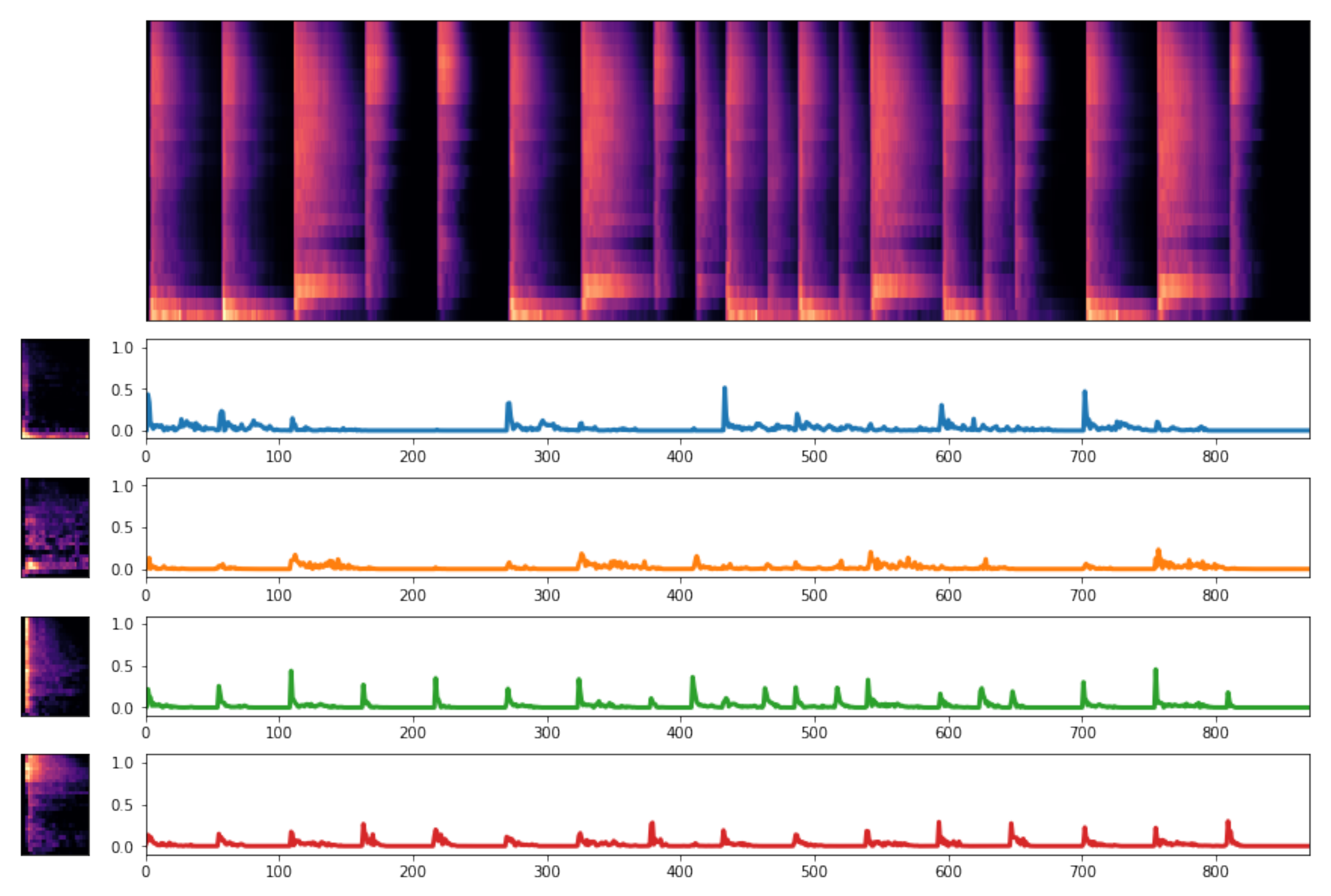
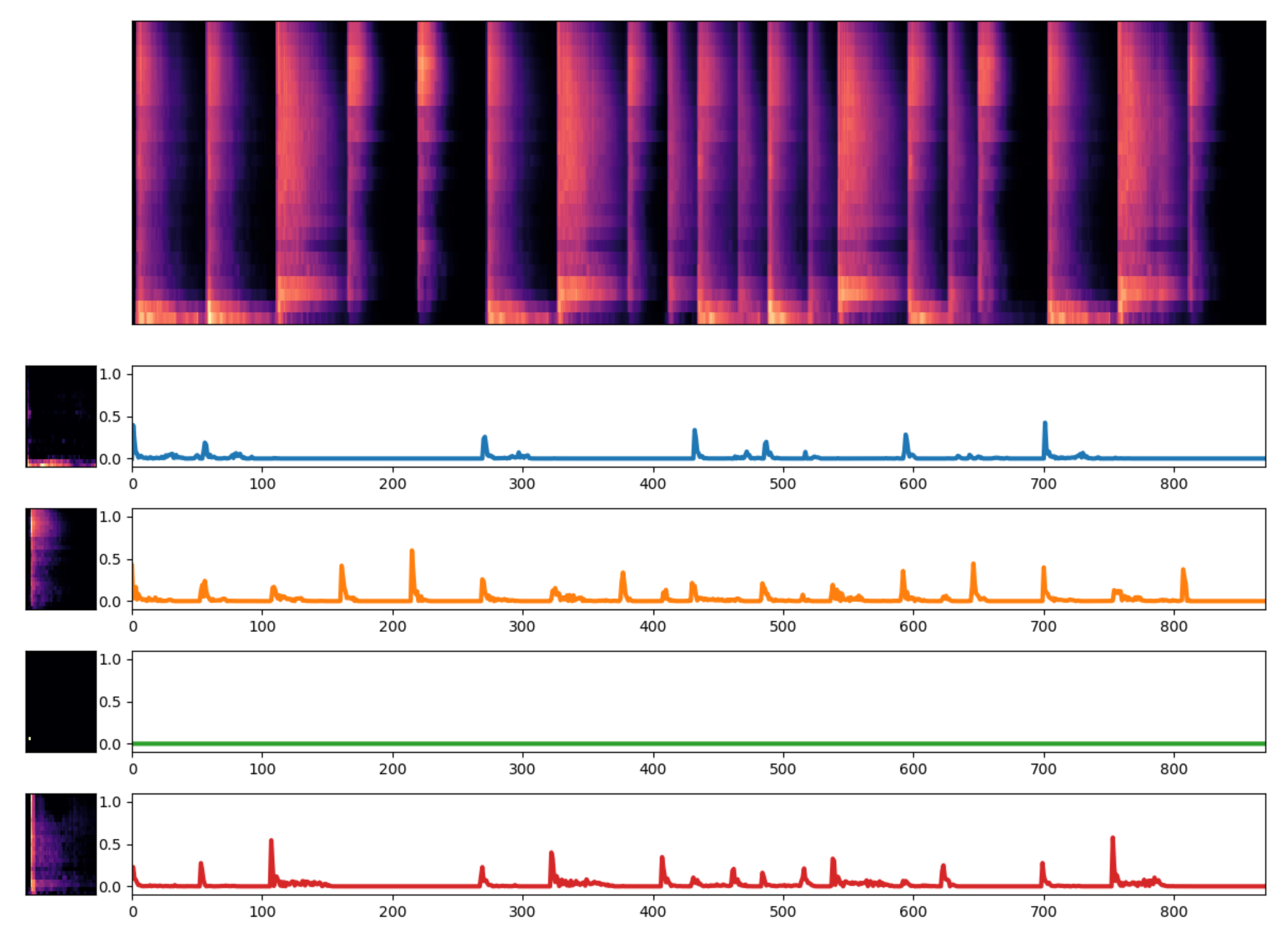
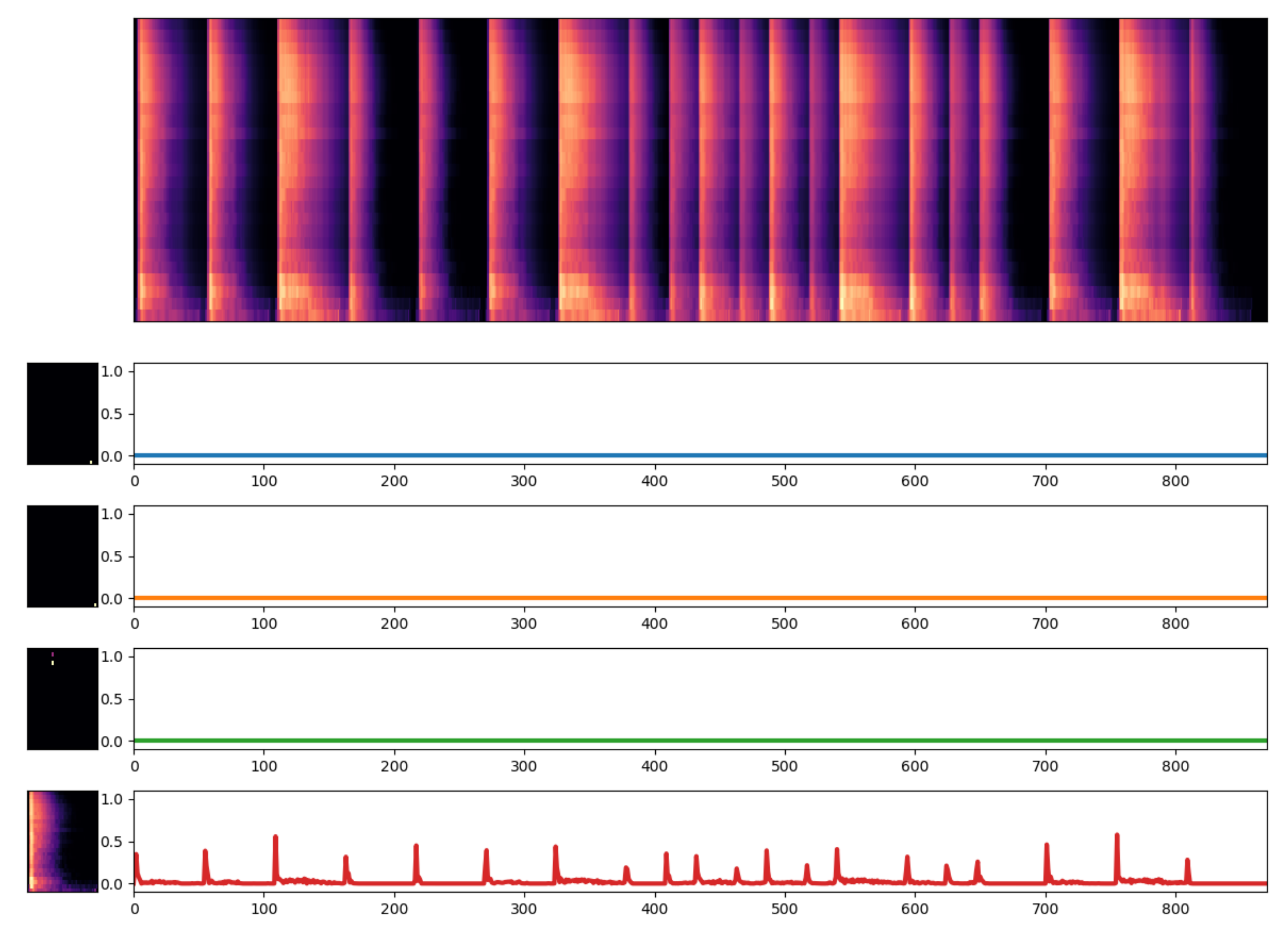
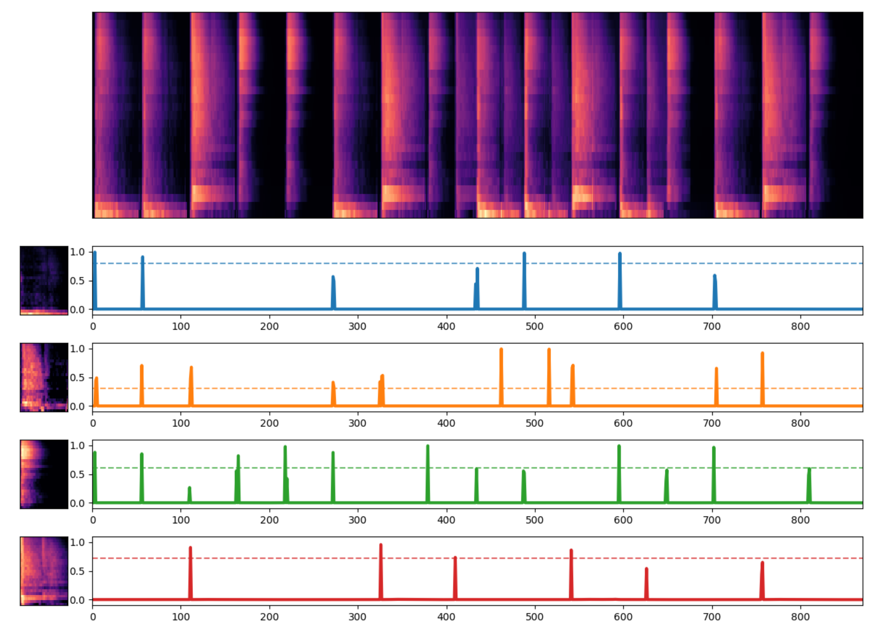
4.3. Example Decomposition

Figure 2 and Figure 4, Figure 5 and Figure 6 show the decomposition of an example drum loop using, respectively, unconstrained NMFD, sparse NMFD with $\lambda =0.1$, sparse NMFD with $\lambda =1.0$, and sigmoidal NMFD (more examples of decompositions are provided as Supplementary Materials to this paper). We do not show the decomposition using the weak sparsity baseline, $\lambda =0.01$, as the results are almost identical to those by the unconstrained model. Note that all decompositions reconstruct the spectrogram approximately equally well, except the reconstruction with high sparsity (Figure 5).

As mentioned in the introduction (Section 1.3), the activations discovered by unregularized NMFD (Figure 2) have two undesirable properties. The first is that the activations are rather “smeared out”, with a sharp initial onset followed by a slowly decaying amplitude. Some small activations are even not preceded by a sharp initial onset, making it hard to determine whether they correspond to a detected drum hit or not. This does not correspond with the expected impulse-like nature of activations of percussive instruments. The second problem is that the activation curves are highly correlated, so that many drum hits are modeled by a mixture of all of the components. This makes it difficult to interpret the resulting decomposition.

When considering the decompositions by sparse NMFD (Figure 4 and Figure 5), it becomes clear that imposing L1 sparsity does not lead to significantly more impulse-like activations. Even more troublesome is that imposing more sparsity by increasing $\lambda$ actually hinders a good decomposition: Figure 5 illustrates that a high $\lambda$ causes all but one of the components to become inactive, i.e., their activations are monotonically zero, in order to minimize the (extreme) sparsity constraint as much as possible. This effect is unfortunately also sometimes observed even for reasonable values of $\lambda$ (Figure 4), so that the effective capacity of the NMFD model is reduced in order to minimize the sparsity constraint.

The aforementioned problems are solved by using the sigmoidal NMFD model (Figure 6). The activations are highly peaked, and each component models distinct parts of the spectrogram. The allocated capacity, i.e., the number of components K, is used effectively, and it is now very clear where specific sounds are repeated in the mixture. It is worth noting that the proposed regularization term ${\mathcal{L}}_G$ only provides a direct bias towards binary “on–off” behavior, and that the impulse-like behavior emerges spontaneously when this bias is applied to the decomposition of a percussive mixture. In this example, the components even lend themselves to a musically meaningful interpretation: the first component captures the low end of the kick drum, the second captures the mid- and high-end of the kick drum and snare drum, the third component captures hi-hat hits, and the fourth component models the snare drum hits. Note that the second component thus contributes to both the kick drum and the snare drum; unfortunately, some entanglement between components is always possible in an unsupervised decomposition. Nevertheless, the decomposition by the sigmoidal model yields much more interpretable results, with activation curves that show to the expected impulse-like behavior.

5. Conclusions

In this paper, we have approached NMFD as an unsupervised decomposition algorithm for percussive music mixtures. Such an unsupervised decomposition is valuable in application scenarios where the exact instruments in the mixture are unknown, or to bootstrap semi-supervised learning approaches such as the one in Wu and Lerch [8]. We investigated an adapted NMFD model where the activations are biased to be binary in nature, by defining them as the output of a sigmoidal function and by applying a regularization term to push their values to saturation. We observe that this results in activations that are highly impulse-like, which correspond to the expected properties of percussive activations, and we have shown that the proposed approach is more effective at obtaining such impulse-like behavior as compared to a sparse NMFD baseline using an L1 sparsity constraint. By means of a case study, we illustrated the potential of our approach to yield more interpretable decompositions.

Regarding future work, we remark that our method, like the original NMFD algorithm, is unsupervised, so that the optimization procedure is free to adapt the templates $W^{\left(k\right)}$ without considering their musical validity. Even in an informed setting, where each $W^{\left(k\right)}$ is initialized with a template of the desired instrument, there is no guarantee that it will converge to a solution where the components map to individual instruments. This issue could be addressed by adding some kind of supervision to the NMFD framework; this could be a supervised learning algorithm that imposes certain musical constraints learned from data, or an interface where a user can guide the decomposition interactively. A related direction for further research would be to investigate other and more informed initialization strategies for the templates $W^{\left(k\right)}$, and to research how the initialization of the templates impacts the outcome of the optimization process. A second limitation is that this work assumes that the number of components K is known in advance. A next step could therefore be to reliably estimate this number of components prior to decomposition, or to use an iterative decomposition strategy, where K is increased progressively until the full mixture has been decomposed. Finally, we propose that the idea of combining a regularization term that encourages diverging activation values with saturating activations could be incorporated in other models and use cases where binary activations are desired, for example, in the context of music transcription beyond percussive recordings, or even for sound event detection in general.

References

1. Dittmar, C.; Müller, M. Reverse Engineering the Amen Break-Score-Informed Separation and Restoration Applied to Drum Recordings. IEEE/ACM Trans. Audio Speech Lang. Process. 2016, 24, 1535–1547. [Google Scholar] [CrossRef]
2. López-Serrano, P.; Davies, M.E.P.; Hockman, J.; Dittmar, C.; Müller, M. Break-Informed Audio Decomposition For Interactive Redrumming. In Proceedings of the 19th International Society for Music Information Retrieval Conference (ISMIR 2018)—Late-Breaking/Demos Session, Paris, France, 23–27 September 2018. [Google Scholar]
3. Wu, C.W.; Dittmar, C.; Southall, C.; Vogl, R.; Widmer, G.; Hockman, J.; Mulleinr, M.; Lerch, A.; Müller, M. A Review of Automatic Drum Transcription. IEEE/ACM Trans. Audio Speech Lang. Process. 2018, 26, 1457–1483. [Google Scholar] [CrossRef] [Green Version]
4. Vogl, R.; Dorfer, M.; Widmer, G.; Knees, P. Drum Transcription via Joint Beat and Drum Modeling using Convolutional Recurrent Neural Networks. In Proceedings of the 18th International Society for Music Information Retrieval Conference (ISMIR 2017), Suzhou, China, 23–27 October 2017; pp. 150–157. [Google Scholar]
5. Southall, C.; Stables, R.; Hockman, J. Automatic Drum Transcription Using Bi-Directional Recurrent Neural Networks. In Proceedings of the 17th International Society for Music Information Retrieval Conference (ISMIR 2016), New York, NY, USA, 7–11 August 2016. [Google Scholar]
6. Southall, C.; Stables, R.; Hockman, J. Automatic drum transcription for polyphonic recordings using soft attention mechanisms and convolutional neural networks. In Proceedings of the 18th International Society for Music Information Retrieval Conference (ISMIR 2017), Suzhou, China, 23–27 October 2017; pp. 606–612. [Google Scholar]
7. Dittmar, C.; Gärtner, D. Real-Time Transcription and Separation of Drum Recordings Based on NMF Decomposition. In Proceedings of the 17th International Conference on Digital Audio Effects (DAFx 2014), Erlangen, Germany, 1–5 September 2014; pp. 187–194. [Google Scholar]
8. Wu, C.W.; Lerch, A. From Labeled To Unlabeled Data—On the Data Challenge in Automatic Drum Transcription. In Proceedings of the 19th International Society for Music Information Retrieval Conference (ISMIR 2018), Paris, France, 23–27 September 2018. [Google Scholar]
9. Smaragdis, P. Non-negative matrix factor deconvolution; extraction of multiple sound sources from monophonic inputs. In Proceedings of the 5th International Conference on Independent Component Analysis and Blind Signal Separation (ICA 2004), Granada, Spain, 22–24 September 2004; pp. 494–499. [Google Scholar]
10. Roebel, A.; Pons, J.; Liuni, M.; Lagrangey, M. On Automatic Drum Transcription using Non-Negative Matrix Deconvolution and Itakura Saito Divergence. In Proceedings of the 2015 IEEE International Conference on Acoustics, Speech and Signal Processing (ICASSP 2015), South Brisbane, Australia, 19–24 April 2015; pp. 414–418. [Google Scholar]
11. Schmidt, M.N.; Mørup, M. Nonnegative matrix factor 2-D deconvolution for blind single channel source separation. In Proceedings of the 6th International Conference on Independent Component Analysis and Blind Signal Separation (ICA 2006), Charleston, SC, USA, 5–8 March 2006; pp. 700–707. [Google Scholar]
12. Lindsay-Smith, H.; McDonald, S.; Sandler, M. Drumkit Transcription via Convolutive NMF. In Proceedings of the 15th International Conference on Digital Audio Effects (DAFx 2012), York, UK, 17–21 September 2012; pp. 15–18. [Google Scholar]
13. Laroche, C.; Papadopoulos, H.; Kowalski, M.; Richard, G. Drum extraction in single channel audio signals using multi-layer Non negative Matrix Factor Deconvolution. In Proceedings of the 2017 IEEE International Conference on Acoustics, Speech and Signal Processing (ICASSP 2017), New Orleans, LA, USA, 5–9 March 2017; pp. 46–50. [Google Scholar]
14. Ueda, S.; Shibata, K.; Wada, Y.; Nishikimi, R.; Nakamura, E.; Yoshii, K. Bayesian Drum Transcription Based On Nonnegative Matrix Factor Decomposition with a Deep Score Prior. In Proceedings of the 2019 IEEE International Conference on Acoustics, Speech and Signal Processing (ICASSP 2019), Brighton, UK, 12–17 May 2019; pp. 456–460. [Google Scholar]
15. Dittmar, C.; Müller, M. Towards transient restoration in score-informed audio decomposition. In Proceedings of the 18th International Conference on Digital Audio Effects (DAFx 2015), Trondheim, Norway, 30 November–3 December 2015; pp. 1–8. [Google Scholar]
16. Liutkus, A.; Badeau, R. Generalized Wiener filtering with fractional power spectrograms. In Proceedings of the 2015 IEEE International Conference on Acoustics, Speech and Signal Processing (ICASSP 2015), South Brisbane, Australia, 19–24 April 2015; pp. 266–270. [Google Scholar]
17. Vande Veire, L.; De Boom, C.; De Bie, T. Adapted NMFD update procedure for removing double hits in drum mixture decompositions. In Proceedings of the 13th International Workshop on Machine Learning and Music at ECML PKDD 2020 (MML2020), Ghent, Belgium, 14–18 September 2020; pp. 10–14. [Google Scholar]
18. Wu, C.W.; Lerch, A. Drum Transcription Using Partially Fixed Non-Negative Matrix Factorization With Template Adaptation. In Proceedings of the 16th International Society for Music Information Retrieval Conference (ISMIR 2015), Málaga, Spain, 26–30 October 2015. [Google Scholar]
19. Virtanen, T. Monaural sound source separation by nonnegative matrix factorization with temporal continuity and sparseness criteria. IEEE Trans. Audio Speech Lang. Process. 2007, 15, 1066–1074. [Google Scholar] [CrossRef] [Green Version]
20. EDM Drums—Drum Samples Kit by ProducerSpot. Available online: https://www.producerspot.com/download-free-edm-drums-drum-samples-kit-by-producerspot. (accessed on 2 December 2020).
21. Gillet, O.; Richard, G. ENST-Drums: An extensive audio-visual database for drum signals processing. In Proceedings of the 7th International Society for Music Information Retrieval Conference (ISMIR 2006), Victoria, BC, Canada, 8–12 October 2006. [Google Scholar]
22. McFee, B.; Lostanlen, V.; Metsai, A.; McVicar, M.; Balke, S.; Thomé, C.; Raffel, C.; Zalkow, F.; Malek, A.; Dana, D.; et al. Zenodo: Librosa/librosa: 0.8.0 (Version 0.8.0). Available online: https://zenodo.org/record/3955228#.YAqsHRZS9PY (accessed on 15 January 2021). [CrossRef]
23. López-Serrano, P.; Dittmar, C.; Özer, Y.; Müller, M. NMF Toolbox: Music Processing Applications of Nonnegative Matrix Factorization. In Proceedings of the 22nd International Conference on Digital Audio Effects (DAFx-19), Birmingham, UK, 2–6 September 2019. [Google Scholar]
24. Code for Sigmoidal NMFD: Convolutional NMF with Saturating Activations for Drum Mixture Decomposition. Available online: https://github.com/aida-ugent/sigmoidal-nmfd (accessed on 12 January 2021).
25. Lee, D.D.; Seung, H.S. Algorithms for non-negative matrix factorization. In Proceedings of the Advances in Neural Information Processing Systems 13 (NIPS 2000), Denver, CO, USA, 29 November–4 December 1999; pp. 556–562. [Google Scholar]
Figure 1. Conceptual illustration of the drum mixture decomposition problem: a percussive mixture (a) is decomposed into prototypical samples of the used instruments (b) and the corresponding onsets (c).
Electronics 10 00284 g001
Figure 2. Decomposition of a percussive recording using non-negative matrix factor deconvolution (NMFD). The activations are not impulse-like, and contain noisy regions where it is difficult to detect individual drum hits.
Electronics 10 00284 g002
Figure 3. Onset coverage F-measure as a function of the peak picking threshold θ thr .
Electronics 10 00284 g003
Figure 4. Decomposition of a drum loop using sparse NMFD, λ = 0.1 . Although slightly more peaked than the activations for unconstrained NMFD (Figure 2), the activations do not show impulse-like behavior, and still contain noisy regions where it is difficult to detect individual drum hit onsets. The third component has become “inactive” in order to minimize the sparsity constraint.
Electronics 10 00284 g004
Figure 5. Decomposition of a drum loop using sparse NMFD, λ = 1.0 . The decomposition fails because the sparsity constraint is too strong, so that only one component remains active.
Electronics 10 00284 g005
Figure 6. Decomposition of a drum loop using sigmoidal NMFD. The activations show impulse-like behavior, and each component captures different parts of the spectrogram, leading to an interpretable decomposition. The dashed line indicates the amplitude a k for each component.
Electronics 10 00284 g006