A Novel Automated Design Methodology for Power Electronics Converters

Abstract

This work proposes a methodology for designing power electronic converters called “Automatic Design for Manufacturing” (ADFM). This methodology proposes creating Power Converter Arrays (PCAs) using standardized converter cells. The approach is greatly inspired by the microelectronics integrated circuit design flow, power electronics building blocks, and multicell converters. To achieve the desired voltage/current specifications, the PCA conversion stage is made from the assembly of several Conversion-Standard Cells (CSCs) in series and/or parallel. The ADFM uses data-based models to simulate the behavior of a PCA with very little computational effort. These models require a special characterization approach to maximize the amount of knowledge while minimizing the amount of data. This approach consists of establishing an experiment plan to select the relevant measurements that contain the most information about the PCA technology, building an experimental setup that is capable of acquiring data automatically and using statistical learning to train models that can yield precise predictions. This work performed over 210 h of tests in nine different PCAs in order to gather data to the statistical models. The models predict the efficiency and converter temperature of several PCAs, and the accuracy is compared with real measurements. Finally, the models are employed to compare the performance of PCAs in a specific battery charging application.

1. Introduction

Design automation in power electronics is a topic that has received much attention in the past years. The main motivations behind the topic are the shortening of product development cycles, the increased use of highly complex power converters, and also the improvement of robustness, resilience, and reliability [1,2].

The automatic design process in power electronics is a hot topic and is discussed today in several research groups around the world [2]. For example, in [3], tools are proposed for assisting the designer choices such as the converter topology selection, the magnetic components design, switching frequency tune, etc. An optimal solution can be obtained with reduced modeling and simulation efforts. Likewise, [4] presents tools for assisting the designer to select the optimal topology, switching frequency, and even the exact components that should be used in order to achieve an optimal solution. In [5], the authors introduce design automation for power modules. The focus of these design methods is on assisting the designer to perform good/optimal decisions during the converter design and to accelerate the design process. However, neither proposes a straightforward automatic process starting from some converter specification to an industrialized product by a complete automatic procedure. In particular, the implementation itself toward manufacture remains most of the time to be done, together with the industrialization process.

Computer-Aided Design still struggles against the lack of standardization in Power Electronics [1]. The sheer number of possible topologies to be considered, together with the amount of components that can be employed to perform exactly the same function and the whole converter design process is so heterogeneous that it is difficult to consider all the parameters and variables that must be considered to accomplish a complete design to manufacture. This is precisely the starting point of the ADFM method proposed in this paper: to contribute to introduce standardization with the objective to perform a fully automated design for manufacturing in Power Electronics.

The Automatic Design for Manufacturing (ADFM) has three main sources of inspiration: The Power Electronic Building Blocks (PEBB), the muticell converters, and the microelectronic digital integrated circuit design process. The ADFM totally rethinks what a power converter is and how to create one. The proposed method sees a power converter as the assembly of standard components rather than a complex design process of a unique solution.

The Power Electronics Building Block (PEBB) methodology formalized the idea that reliability can be improved while reducing costs by using standard building blocks in the design of power electronics converters [6,7,8,9,10,11,12]. The methodology streamlined the conception of converters with high power density, efficiency, and reliability [13,14]. It achieved scalability, high voltage operation, repairability, and reliability. Nevertheless, the idea of an automated design process and the missing link between microelectronic and power electronics, which were pursued in its initial publications [6], are less present in its actual state of the art. The most notable low and medium power/voltage converters based on standardized subsystem are the power modules and IPEM (Integrated Power Electronics Modules) [15,16].

Multicell converter topologies and architectures give also inspiration to the automated design of power electronic converters. The “multicell” terminology was first employed in the 1990s, as illustrated in [17,18] to call for what today is named a flying capacitor converter. The technique was initially focused on performing high-voltage power conversion and started to be implemented in multiple high-power applications [19]. In the early 2000s, “multicell converter” was also referring to any converter topology made out several conversion cells [20]. More recently, thanks to the increase in performances and characteristics of low-voltage power devices such as MOSFETS but also wide band gap devices, and their associated gate driver stages, multicell converters are also implemented in medium and low-voltage applications to benefit from the multicell properties to design more efficient converters [21].

The ADFM method proposes combining PEBB principles and multicell converters conversion techniques with microelectronic digital integrated circuit design and manufacturing workflow. Digital electronics design and manufacturing flows have allowed creating very complex systems and devices, integrating in one single chip billions of transistors while providing extremely high levels of reliability, constrained costs, and overall production efficiency. Despite the differences between microelectronics and power electronics, the digital synthesis approach, based on the automated and generic association of standardized cells, offers a great illustration of how power electronics converters design methods could be inspired.

In contrast with most of the methods presented in [1], the ADFM method does not aim to create an optimal solution for a converter. Instead, it proposes a viable solution, with a reliable prediction of efficiency and operating temperature. The performance levels of the designed converter are not defined by a careful optimization at converter-level design but by an overall optimization of the technology platform (TP) characteristics, which are in turn used in the converter design process [22,23].

The contribution of this paper lies in presenting the main steps of the ADFM methodology and the process it follows to automatically create a power converter. Another important achievement of the ADFM method is the accurate prediction of the performance (efficiency and temperature) of converters through virtual prototyping. This paper details the construction of statistical models based on machine learning algorithms to predict the converter’s performance and how to acquire a relevant dataset to train these algorithms. The statistical models can be used to determine the performance of a converter in every point of operation of a mission profile. For that purpose, the presented work assumes that a technology platform is already available, containing all necessary standard cells to build a PCA. In such a sense, the paper is not focused on the optimization of the PCA performances or characteristics. It is strictly focused on the design method and then selects the best compromises from a set of possible solutions.

This paper is organized as follows. Section 2 briefly introduces the technology platform concept, through its analogy with digital electronics design flow. Section 3 describes in detail the ADFM methodology to create a power converter from standard cells. In order to acquire knowledge on the standardized cells, which the methodology assembles to create converters, there is a long process of characterization and construction of a database. The main steps of this process are presented in Section 3. Once the data that describes the standard cells, as well as their associations, are acquired, Section 4 presents the machine learning algorithms used to train statistical models describing the main characteristics of any PCA designed from these standard cells. Section 5 presents some practical use of the models, which were used to predict the behavior of the converters created by the ADFM methodology, at any operating points.

2. The Technology Platform

In a comparable process with digital design in microelectronics, the ADFM method in power electronics consists in assembling and interconnecting standard cells to create Power Converter Arrays (PCA). A PCA is an assembly of well-known and reliable standardized elements, or Standard Cells (SC). These standard cells are constructed within a technology framework, which follows a rigorous maturation process that ensure an optimal performances and industrialization readiness. The PCA can be divided in two parts: a power conversion stage and a control stage.

The power conversion stage of a PCA is made by the assembly of Conversion-SCs (CSC) associated with Terminal-SCs (TSC), corresponding respectively to the front end and the back end in microelectronics. The SC cannot be modified from one design to another, so, the way these cells are physically arranged and electrically interconnected are used to determine the power electronics work function (step up, step down, multiple outputs, single three, or multiphase conversion). A variety of CSCs are needed to answer the various functions to be implemented in power electronics (DC to DC, AC to DC, bidirectional current, galvanic isolation or not, etc.). In addition, the same technology platform may integrate several CSC families with the same functionalities but for different voltage or current ratings.

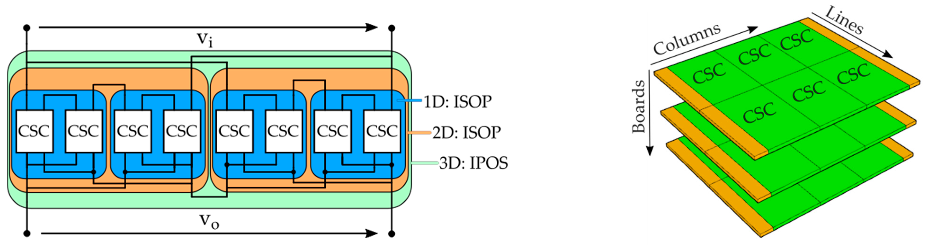
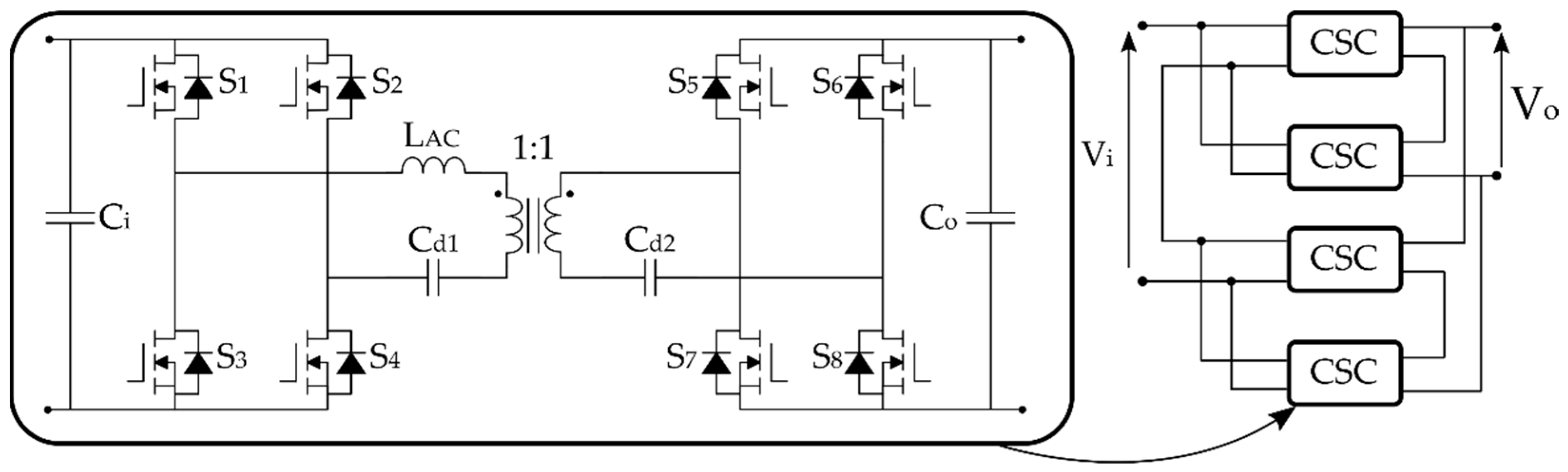
In order to create PCAs with different voltage and current conversion ratios, CSCs are associated in four different types of configurations: Input series output series (ISOS), input series output parallel (ISOP), input parallel output series (IPOS), and input parallel output parallel (IPOP). Figure 1 (left) presents the schematic of a PCA made from eight CSCs, which were connected with three levels of configuration. The physical arrangement, which in the context of this work is named architecture, can be made in lines, columns, and/or boards, as presented in Figure 1 (right).

The “control” stage contains Measurement-SCs (MSC), Protection-SCs (PSC), and Control-SC (CoSC). The SCs presented in the control stage are highly dependent on the application, on how many measurements are required (voltage and/or current), the type of protection, etc. Details about the control stage SCs are out of the scope of this publication.

The specifications of a technology platform are always larger than the one of a specific converter. It includes a set of generic characteristics, such as standard and regulation compliance, some technology constraints, such as available cooling, interconnection, and assembly techniques, some performances goals such as targets on space for which design of PCA are possible, such as the range in input/output voltages and currents, range in dynamics, etc.

ADFM automated design uses algorithms to find solutions to configure and to assemble the various standard cells necessary to fulfill some given converter specifications. Similar to the microelectronic integrated circuit synthesis, the models that describe how families of SCs behave are data-driven statistical models based in real experiments. The creation of these models is presented in the following sections of this work.

3. The Automated Design for Manufacturing (ADFM) Method

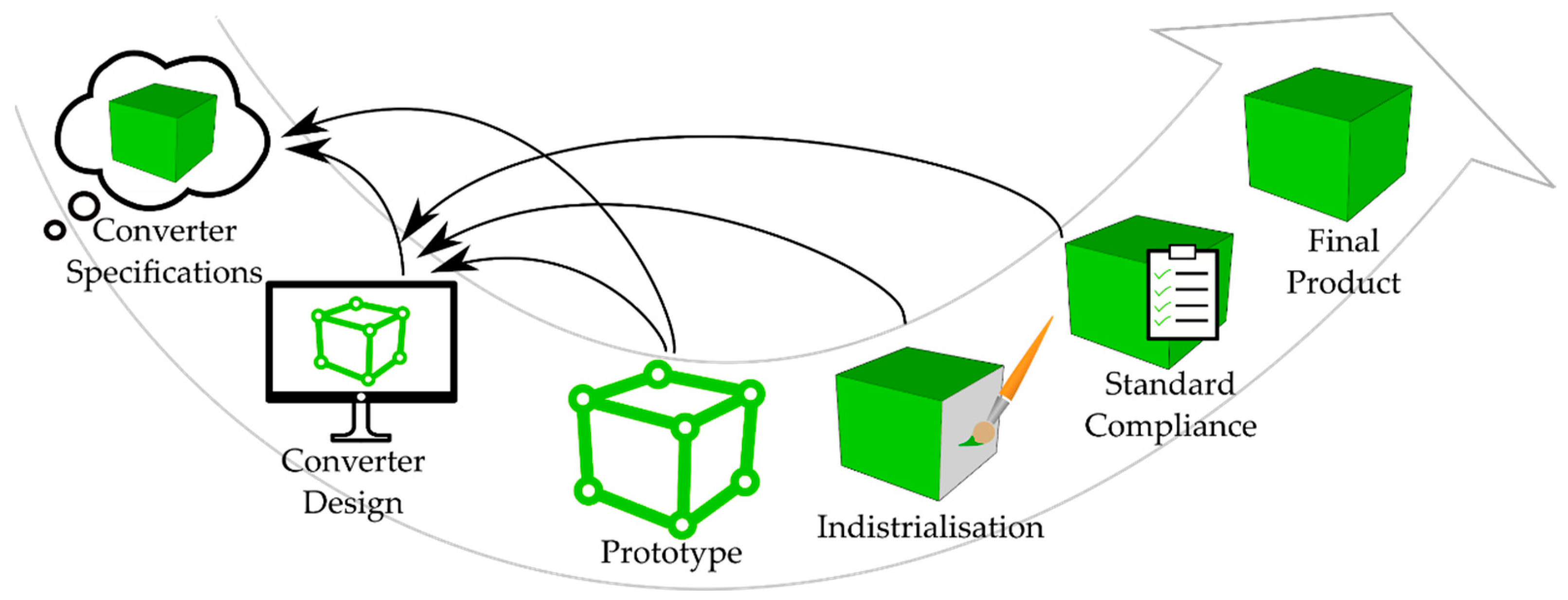
Power electronic converters are traditionally designed following several steps as presented in Figure 2, the steps consist of the following:

Defining the converter specifications: The converter specifications must be clear, well defined, and evaluated and approved by the lead designer as a feasible request. All specifications, including the function to be performed, power and/or current and/or voltage levels, expected dynamics, the converter operating conditions such as ambient temperature, and ambient thermal cycling are fundamental. It also includes application field requirements such as efficiency, power quality, power density, price, complexity, and standards compliance.

Converter Design: The designer chooses the circuit topology, the modulation scheme, the control strategy, and the types and ratings of the components together with the switching frequency. An important issue is related to the interconnect and assembly technologies to be chosen together with the cooling. These choices have a significant impact on converter performances and characteristics such as power densities or efficiency. Then, the designer must take care of the physical arrangements of the converter and the positions of the components. Housing, cooling techniques, and packaging must be defined according to operating and implementation conditions. This stage also includes electrical and/or thermic simulations to tune some design parameters.

Prototype: A prototype is usually built and implemented to verify if the design and choices are in accordance with the specifications and the targeted performances. If the specifications are not achieved, or if the performances are below expectations, the designer must take some steps back and carry on a rework on the design itself and the decisions made.

Industrialization: The industrialization process purpose is to verify the component selections and sourcing to achieve lower costs and higher availability. The manufacturing complexity is verified, and the layout and position of components may be modified to ease the assembly process. In addition, tests to evaluate the converter reliability are performed. Accelerated aging tests are made to verify that it complies with specifications over a certain period of time.

Standard compliance: Then, the power electronic (PE) converter must be tested for standard and regulation compliance before entering in mass production.

Once this process is completed, the price for the PE converter can be set. Its main characteristics can be accurately determined, such as its power density, efficiency, and reliability.

As it has been described above, the design process of a PE converter is a complicated and multidisciplinary process. Several tools have been developed to help in the design process. Among them, circuit and control simulation software are specific and essential. In addition, multi-physics software such as thermal and fluid simulation, finite element modeling, and electromagnetic interference analysis are regularly considered to help the designer in its optimization process. Nonetheless, the full design process requires many hours of work, involving various specialists from different fields. As a matter of fact, the design process of a brand-new converter is expensive and time consuming.

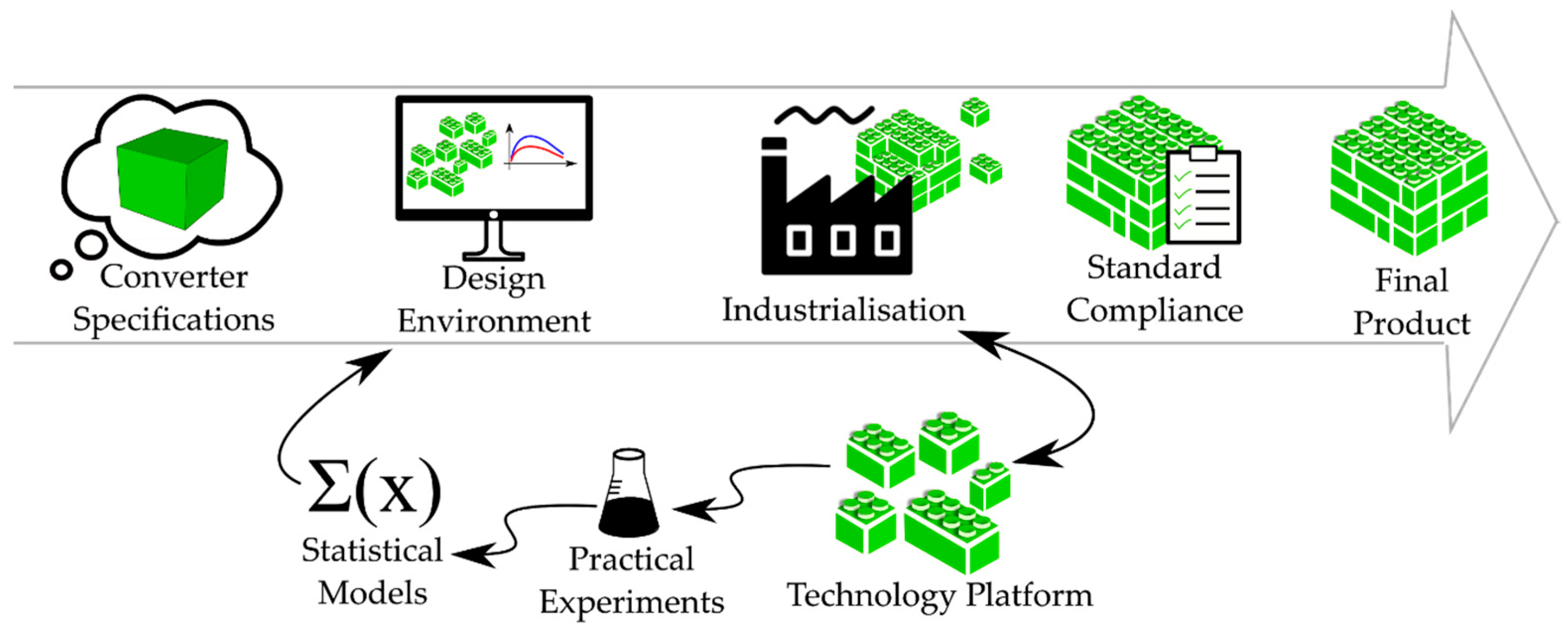
In opposition to the traditional method, the ADFM presented in Figure 3 proposes a completely inverse logic to design a converter. Prior to running a complete ADFM, a set of technology platforms must be made available to cover a wide range of options, applications, and targeted performances. Once each of these technology platforms are well characterized and modeled, a database is built for each of them with many parameters and characteristics made available for the design and selection routine. Based on machine learning and statistical modeling, the characteristics are extracted from existing and representative PCAs and CSCs, providing accurate prediction models.

Based on these highly accurate models, a very linear and straightforward design and selection approach can be carried out from the specifications of the desired power converter through a virtual prototyping phase. First, the converter specifications are compared to the characteristics of each technology platform. Then, possible solutions are identified in each phase of the TP compliance. Various configurations and architectures are virtually prototyped to identify the one with the best characteristics. In the space of all possible solutions, the designer tunes the design and selection parameters to identify the best option to be afterwards produced. Since all this process is only able to select interconnections and assemble standardized cells that are built to be interconnected and assembled, there is no custom design carried out. The resulting PCA converter is the optimal solution that the given TP can provide. The virtual prototyping phase also allows knowing in advance that it will be possible to produce it in volume, and it is also possible to predict accurately its main characteristics such as efficiency, power densities, thermal cooling needs, and even compliance with regulations. It is expected with such a design approach to be able to run a first prototype that will directly meet all specifications as long as these specifications are feasible under the TP characteristics.

This paper is now going to focus on the characterization stage of the power part of the PCA, with the objective to tune predictive models able to forecast efficiency and converter temperature with respect to specifications, which are the cornerstone of the virtual prototyping that the proposed method is built upon.

4. Design of the Experiments and Experimental Setup

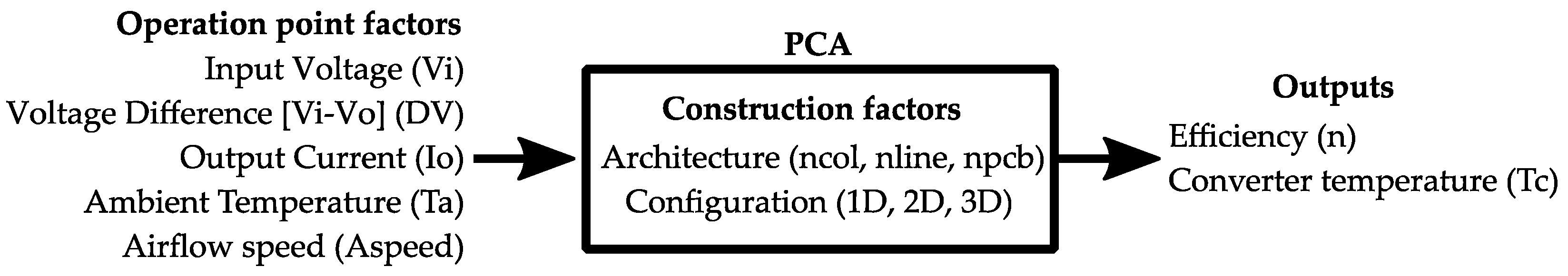
The ADFM method presented in this paper uses two figures of merit as design and selection criteria for PCAs: efficiency and the thermal characteristics. The thermal behavior of a PCA can be represented by its global operating temperature. The PCA operating temperature is directly related to generated losses and heat removal capabilities that need to be set. Operating temperature and efficiency are linked by PE converter losses, making both of them critical output variables to be considered by the designer to create a converter that will comply as much as possible with the specifications.

The input variables that affect the output variables were divided in two groups: the operating point variables (voltages, currents, cooling parameters such as ambient temperature and airflow rate) and the construction variables (architecture and configuration), as they were defined in Section 2. While dealing with multi-dimensional experiments, a commonly used procedure is a design of experiments (DOE). A DOE aims to define experiments to be carried out with the objective to maximize the amount of information gathered for a given experimental effort [24]. This work decided to apply DOE techniques individually to the operating point variables and to the construction variables because the former group can be easily studied with a prototype and the latter consists of building up different prototypes. An overview of all the input and output variables is presented in Figure 4.

A technology platform is designed to cover a range of electrical and thermal specifications of certain application field. The TP studied in this work is designed to cover the range presented in

Table 1. The Technology Platform main characteristics.

Parameter	Value/Detail
Input and Output Voltage Range	12 V to 600 V
Current Range	Up to 90 A
Dielectric Isolation	1.5 kV
Assembly and Interconnection Technology	PCB
Cooling Technology	Natural convection or forced air

. Details about the Conversion-Standard Cell studied in this work are presented in

Table 2. Details about the Conversion-Standard Cell (CSC) used in this work.

Parameter	Value
Maximum Input Voltage	20 V
Minimum Input Voltage	8 V
Maximum Output Voltage	20 V
Minimum Output Voltage	8 V
Maximum Output Current	5 A (Highly dependent on cooling factor)
Dimensions (Length, Width, Height)	(24 mm, 47 mm, 13 mm)
Insulation	1.5 kV
Weight	30 g
PCB Maximum Temperature	90 °C

. It consists of a Dual Active Bridge topology, operating with phase shift modulation, as illustrated in Figure 5.

4.1. Preliminary Study of the Operating Point Variables

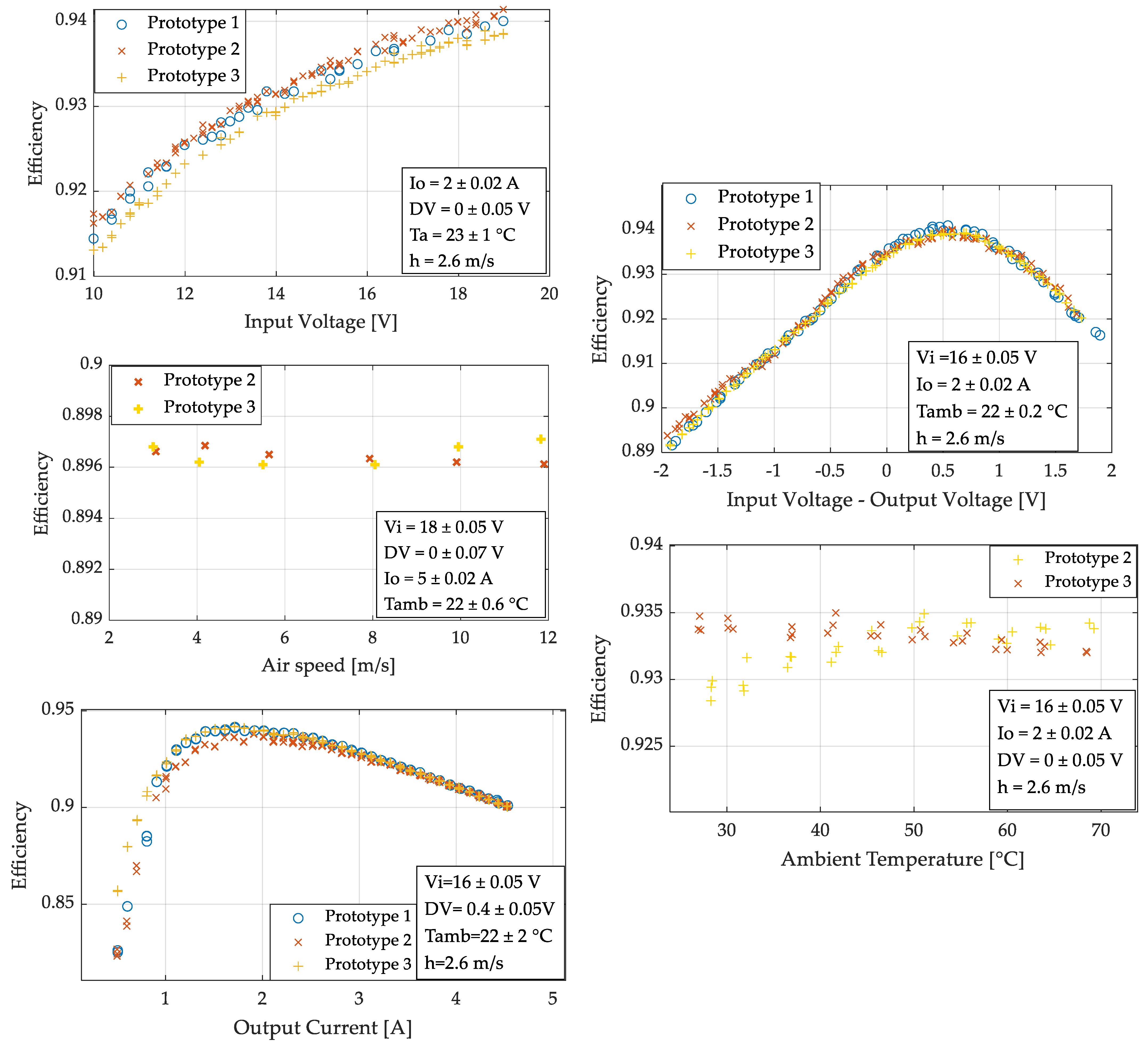
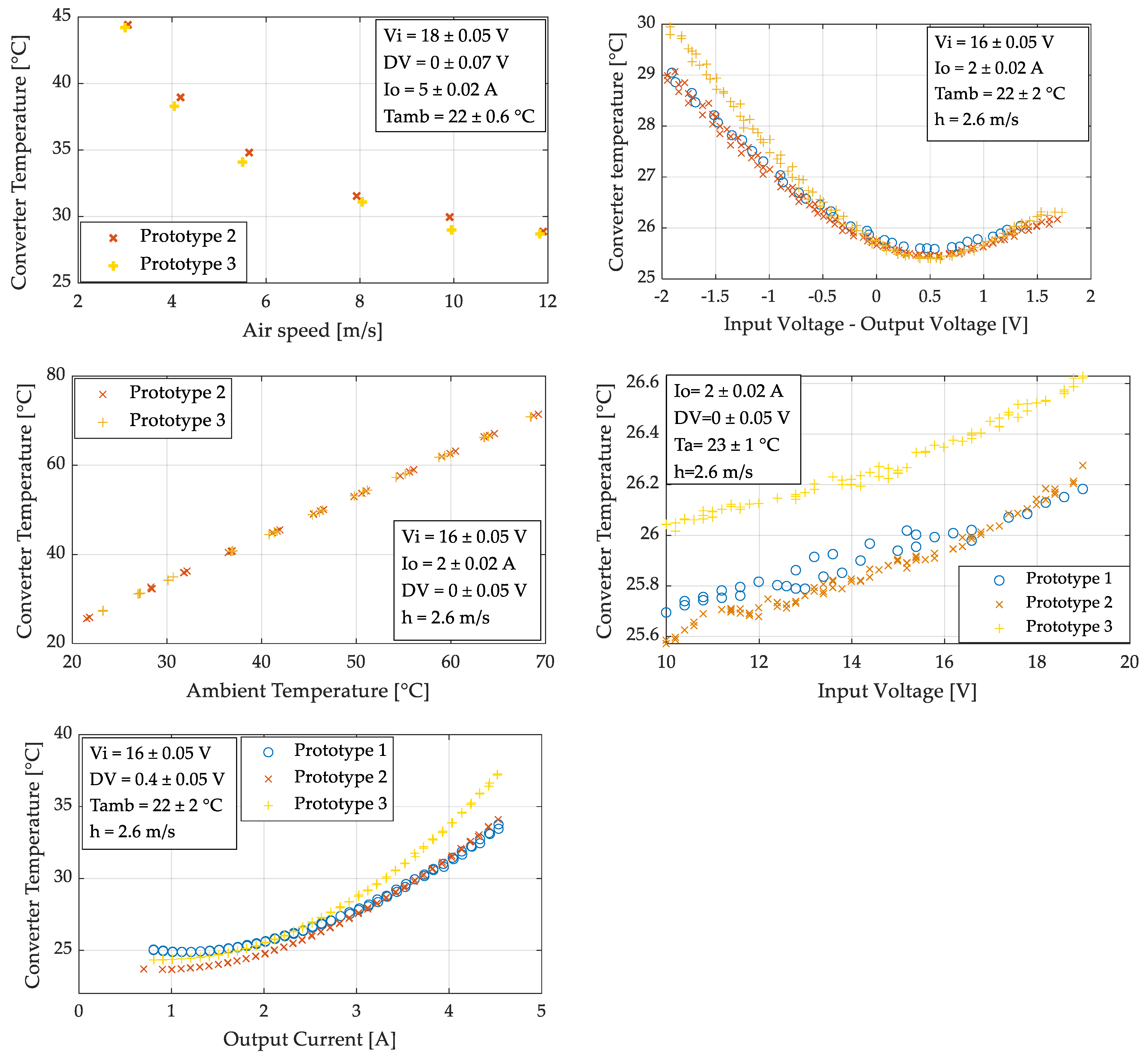
The two output variables that will be analyzed for every operating point of every possible PCA are the PCA efficiency and PCA maximum operating temperature. After a theoretical overview of which variables impact the efficiency and the temperature of the converter, this work defined the operation point of the PCA with five input variables: Output Current (Io), Input Voltage (Vi), Output voltage (Vo), Ambient Temperature (Ta), and Airspeed flowing through the converter (Aspeed).

In order to create a DOE, a primary set of tests was performed with three identical PCAs containing one CSC. These tests consisted in varying one variable at the time in order to identify the shape of the response each input variable induces in each output variable. Once the shapes of the responses are known, it is possible to select a minimum quantity of values for each input variable in order to set up a DOE that is accurate and representative enough of the tendencies.

Figure 6 and Figure 7 present the results of this primary set of tests. The variable Output Voltage (Vo) is expressed by DV, which is the difference between the input voltage and the output voltage (Vi-Vo).

To decide how many levels an input variable should have in the DOE, the general response of each output variable with respect to each input variable must be interpreted. Roughly, three types of responses are expected: a linear, a quadratic, or a more complex response. A linear response can be easily modeled by two levels. A quadratic can be represented by three levels. A more complex response should be modeled with four or more levels. In order to extract as much information as possible about the behavior of the variables, the levels must be selected around maximum, minimum, or inflexion points [24].

After analyzing the results of the experiments presented in Figure 6 and Figure 7, the levels for each input variable selected are presented in

Table 3. Operating points in which the PCAs will be tested in a full factorial experiment.

Operating Point Study
Variable	Vi [V]	DV [V]	Io [A]	Aspeed [m/s]	Tamb [°C]
Range of variation	10 to 20	−2 to 2	0 to 5	0 to 12	20 to 70
Chosen operating point	[10; 14; 18]	[−1; 0; 0.5; 1; 1.5]	[0.75; 1.5; 2; 3.5]	[2; 4; 8]	[30; 55]

.

Opposed to the experiment “one variable at a time”, a full factorial test consists in testing all possible combinations among the selected levels. The individual effects of each input variable over each output variable are extracted. In addition, the coupling effects of two or more variables over each output variable can be highlighted. Table 1 summarizes the main levels selected for the first experience. With these selected points, the factorial test results in 360 experimental points to be carried out.

4.2. Construction Variables

Prototypes are expensive. However, construction variables are totally dependent on the hardware itself to reflect the effect of architecture and interconnection. Then, the DOE must indicate the minimum number of prototypes that best reflect these variables.

The prototypes have been built in order to enable different PCA configurations with the same hardware, acting on the power interconnections with jumpers. In such a way, the DOE can be divided into sequences: defining which prototypes to be manufactured to set the studied “architectures” and defining which power interconnections to be made in order to take into account various configurations.

As presented in Figure 1, the architecture consists of three variables representing the physical arrangement of CSC in a 3D space: the number of lines (nline), number of columns (ncol), and number of boards (nboard). These variables are independent. The CSC technology chosen for this work is limited to nline = 5, ncol = 5, and nboard = 2. Still, this makes 5 × 5 × 2 = 50 possible architectures. Ideally, nline, ncol, and nboard should be studied independently, but the Printed Circuit Boards (PCB) manufacturing process is cheaper when done in quantity. The cost of the experiment is reduced when identical boards with a given ncol and nline are constructed and then stacked up to form a ncol × nline × 2 and ncol × nline × 3.

In this work, the number of columns is clamped to five in order to keep the current flowing through the power interconnections below their maximum ratings. This is especially critical for parallel associations were the current supported by the interconnection element in our technology is limited to 30 A. So, five conversion cells in a line, connected in parallel working at 5 A each, would result in 25 A, which is more than 80% of the interconnection element limit. Of course, it would remain possible to design PCAs with up to 10 columns with the CSC operating at 3 A max or even 30 columns with the CSC limited at 1 A. In this work, the boundaries are set at five lines, five columns, and two boards in order to squeeze prototyping costs.

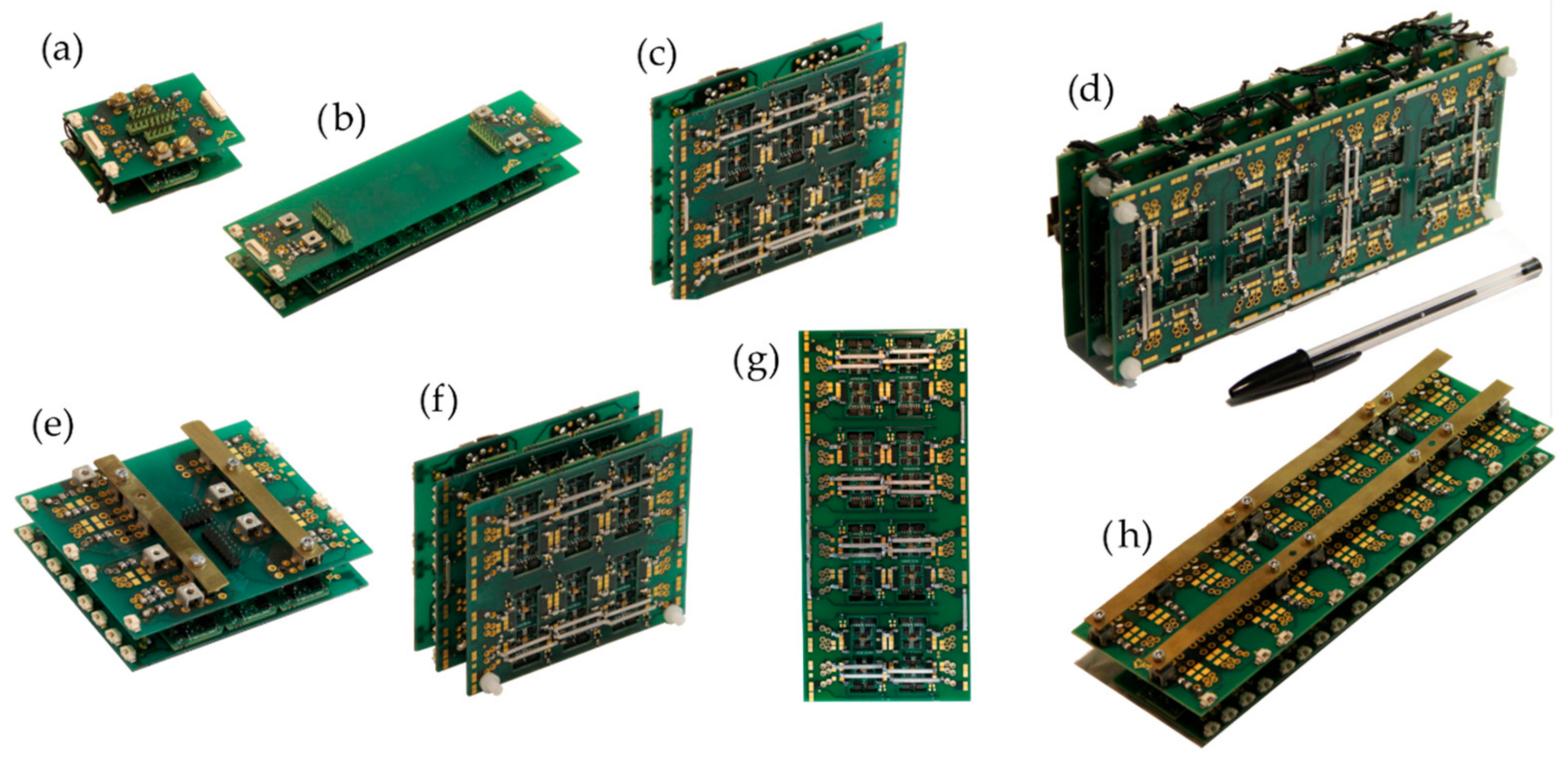
In order to define which PCAs are manufactured and implemented for testing, the number of columns and the number of lines are the only variables that are analyzed. Since both can vary from 1 to 5, there are 25 possible choices. Among the possibilities, six have more than 14 conversion standard cells: these PCAs would amplify the complexity of the experiments because they would require a test bench equipped with larger power supplies and electronic loads. Among the 19 remaining solutions, it was decided to do a sampling that contains at least one board containing 1, 2, 3, 4 and 5 lines and 1, 2, 3, 4 and 5 columns. The selected boards chosen to be fabricated are (nº of lines, nº of columns): (1,1); (5,1); (2,3); (4,2); (3,4); (1,5).

As two identical boards, among the selected one, can be stacked, there are 12 different architectures to be tested. Each one has one to three dimensions (as presented in Figure 1) and can be connected either in ISOP, IPOS, IPOP, or ISOS. This work profits from the natural balance mechanism that ISOP and IPOS converters present as illustrated in [25] and will perform tests only with these two types of connections. All PCAs that were tested are presented in Figure 8.

4.3. Automated Test Bench

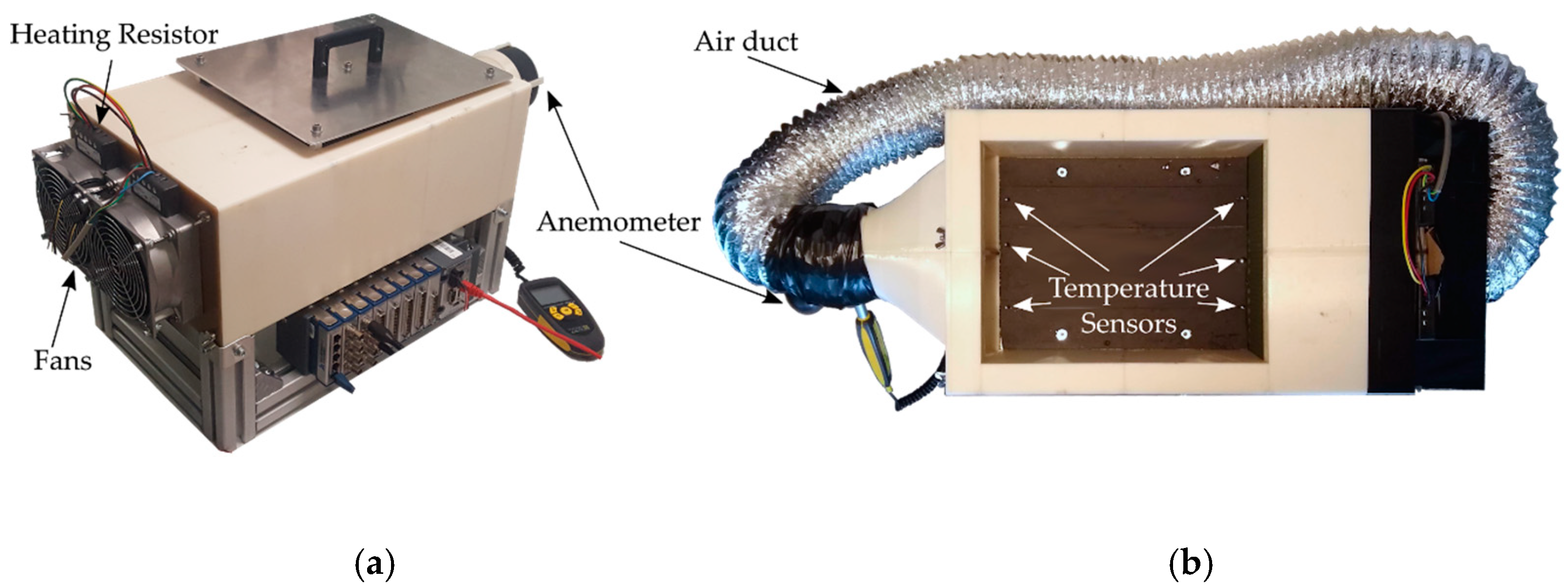
Due to the high number of experiments, an automated test bench was constructed. This test bench consists of a controlled environment wind tunnel, which has fans on one side and an anemometer on the other. Right after the fans, there are heating resistors that can heat up the air, emulating ambient temperatures from room temperature up to 70 °C. The interior of the wind tunnel has six temperature sensors. The device is presented in Figure 9. All data are sent to a computer where all devices can be controlled by a LabVIEW system. In addition, a power source and an electronic load are controlled in order to apply the desired voltage/current in the input and output of the PCAs. The inside shape of the tunnel can be adapted in order to present a cross-section that is identical to the one of each PCA. In such a way, the air force is channeled properly into the PCA, as it would be the case in the specific housing with dedicated fans.

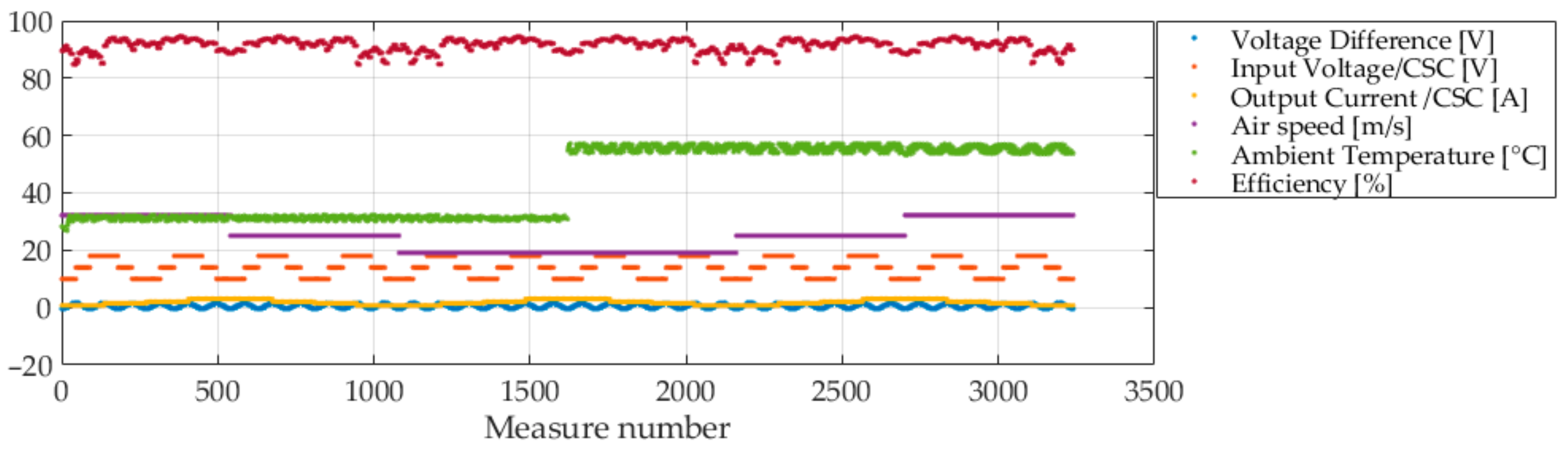
In this work, the experimental setup followed the ranges defined in the DOE to the extent of the precision of the sensors in the wind tunnel. Figure 10 presents a complete experimental characterization cycle for one PCA. In total, 360 different operating points were tested, and for each of them, nine measurements were repeated and averaged. The total number of measurements per variable and per characterization cycle is 3240, representing about 30 h of tests per PE converter.

5. Experimental Results and Statistical Models

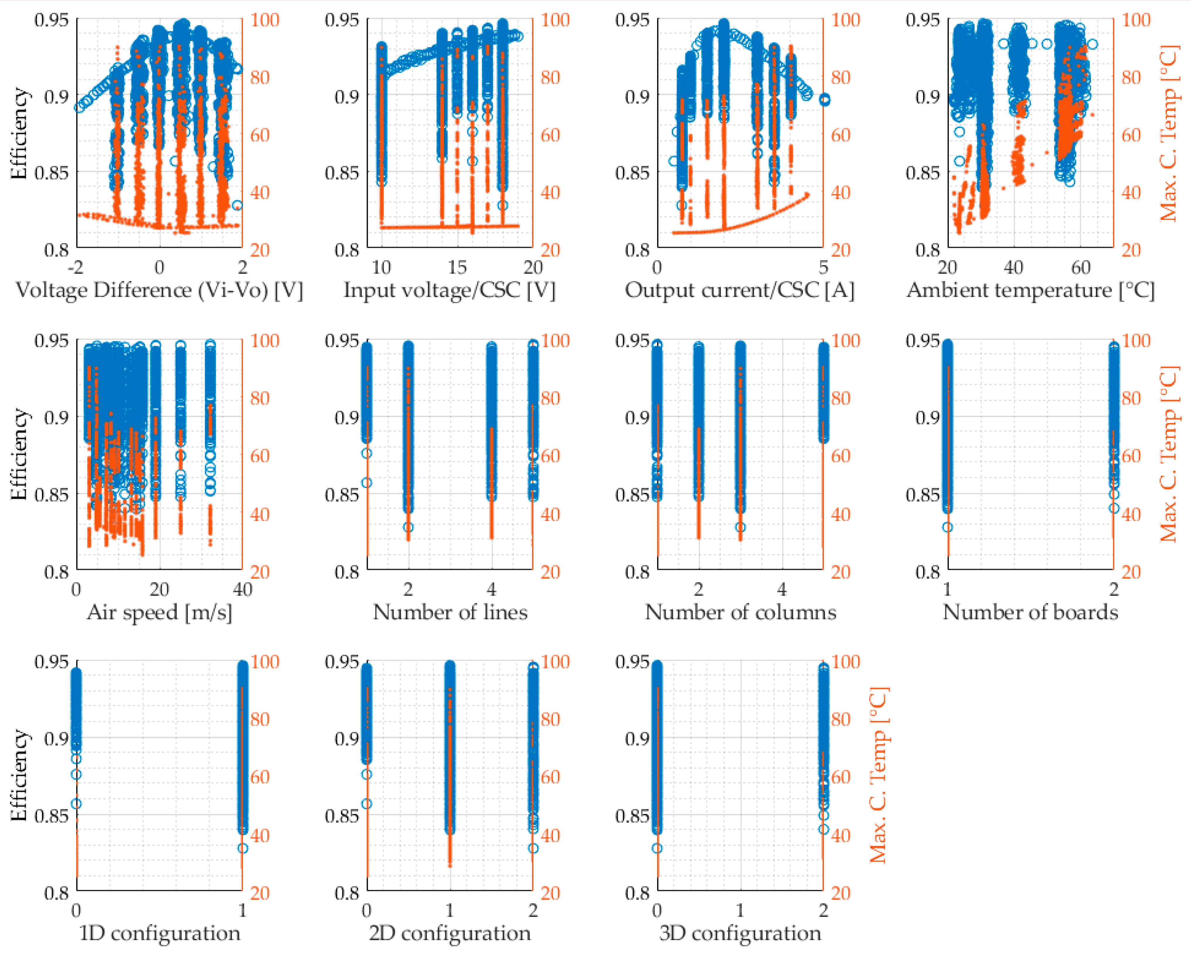
After performing the experimental procedure in the eight chosen PCAs, 2548 measurement points were obtained. Each operating point was repeated nine times, resulting in a total of 22,932 measurement points. In order to reduce the equipment measurement errors, this work used the average value of the nine repetitions. The complete dataset with 2548 experiment points is displayed in Figure 11. The eleven plots present each input variable as a function of the two outputs: efficiency in the left y-axis and converter temperature in the right y-axis. The data acquired in Section 4, in the one variable at a time test, are also added to the dataset.

Statistical modeling uses real-world variables, bundled in datasets, to train mathematical models and make predictions with a certain degree of confidence. This work aims to build/fit a model capable of predicting the efficiency and the temperature of a PCA for the 11 input variables presented in the last section. As both output variables are continuous, this is a typical regression problem.

There are many modeling techniques to build a regression model. Typically, they can be divided in parametric models and non-parametric models [26]. Parametric models can be easily used when the relation between input and output variables are already known to the user; e.g., the temperature of the converter varies linearly with the ambient temperature, or the efficiency has a 1/x relation with the input voltage. However, when dealing with many input variables and some with behaviors that are hard to guess, the parametric models became prone to bias error [26].

In contrast, non-parametric models make no assumptions about which mathematical function best models the data. These models use the whole dataset as input to a non-interpretable algorithm/equation that aims to predict as close as possible the output data without being too wiggly or rough [26]. As these methods make no pre-assumption about the function shape, non-parametric fits can model a wide variety of shapes, making the modeling process much more straightforward, especially in multi-dimensional problems. However, these non-parametric methods required more data than parametric models to obtain precise predictions, and usually, it is impossible to interpret the result.

Gaussian Process Regression (GPR) is a particular type of non-parametric model. Considered sometimes as a meta-parametric technique (or semi-parametric), the GPR does not have physical parameters as parametric models, it has so-called hyper-parameters that grant the user some degree of tuning. The benefits of the GPR method are that no prior knowledge about the shape of the response is required, making it robust against the bias error as other non-parametric methods. In addition, it is still robust if only a small dataset is available for training.

This work opted to use the Gaussian Process Regression (GPR) to create the models for predicting the converter efficiency and temperature. This technique has already been applied in a few topics in the electrical engineering field such as in [27] to predict the health of batteries, in [28] to estimate the lifetime of IGBT devices, and in [29] to create models of the switching process of MOSFETs.

The GPR method create a model that mathematically assures a minimal error of the prediction if the appropriate kernel and its associated meta-parameters are used. For the sake of brevity, mathematical details on GPR are not presented in this work; the reader is invited to read more in [27,28,29,30]. In order to fit a model using the GPR method, it is required to find which kernel best suits the problem under study [30]. This work opted for exploring four classic GPR kernels suited for non-linear systems: exponential (EX), Matern 5/2 (M52), rational quadratic (RQ), and squared exponential (SE). The k-fold cross-validation was used to fit (with k = 5). Their root means square error (RMSE) and training time are presented in

Table 4. The root mean square error and training time of each model and its correspondent kernel both for the efficiency and temperature.

	Efficiency Models		Temperature Models
Kernel	RMSE [Points of Efficiency 10−3]	Training Time [min]	RMSE [°C]	Training Time [min]
Exponential (EX)	2.85	28.9	2.22	7.6
Matern 5/2 (M52)	1.27	23.9	16.34	5.2
Rational Quadratic (RQ)	1.34	22.1	7.46	12.4
Squared Exponential (SE)	1.43	12.9	5.96	4.7

.

The value of the RMSE displayed in Table 2 represents the training error of the models, or how close the predictions are to the estimated results used through the training process. These values do not necessarily demonstrate how good the predictions are but instead indicate how close these are to the training data overall. The data used to train the model can be used to carry out some initial analysis of the accuracy of its results. Still, the validation of the model must be done with an independent set of data.

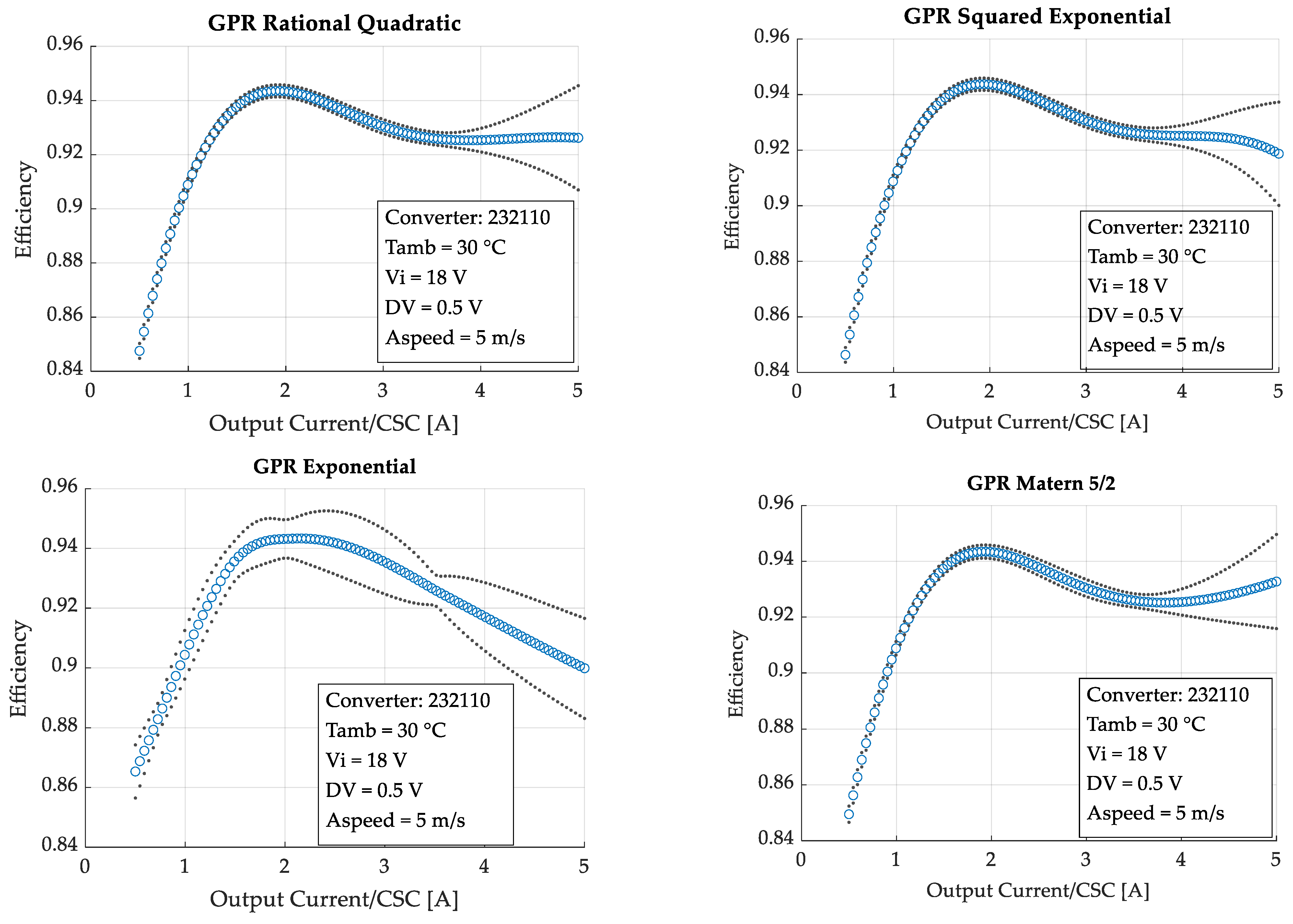
A primary evaluation of the quality of the prediction of each kernel can be made by comparison between the predictions and some well-known physical characteristics of a power converter. To perform this comparison, Figure 12 presents the models predictions of the efficiency of a PCA (two lines, three columns, two boards) as a function of its output current. All operating point variables, despite output current, are kept constant, and their values are displayed in the box inside each respective plot. The gray dots represent the 95% confidence region of the prediction, while the blue dots show the actual predicted values.

It can be seen in Figure 12 that the models trained with kernels M52, the RQ, and the SE present high accuracy until 3.5 A, which is the region in which most of the training data is concentrated. Past this current, these kernels have physically incoherent results. Only the EX kernel presents physically coherent results after 3.5 A; however, it has a higher incertitude than the other three kernels in predictions with lower currents. Depending on the predicted point, one kernel or another can be used for best results.

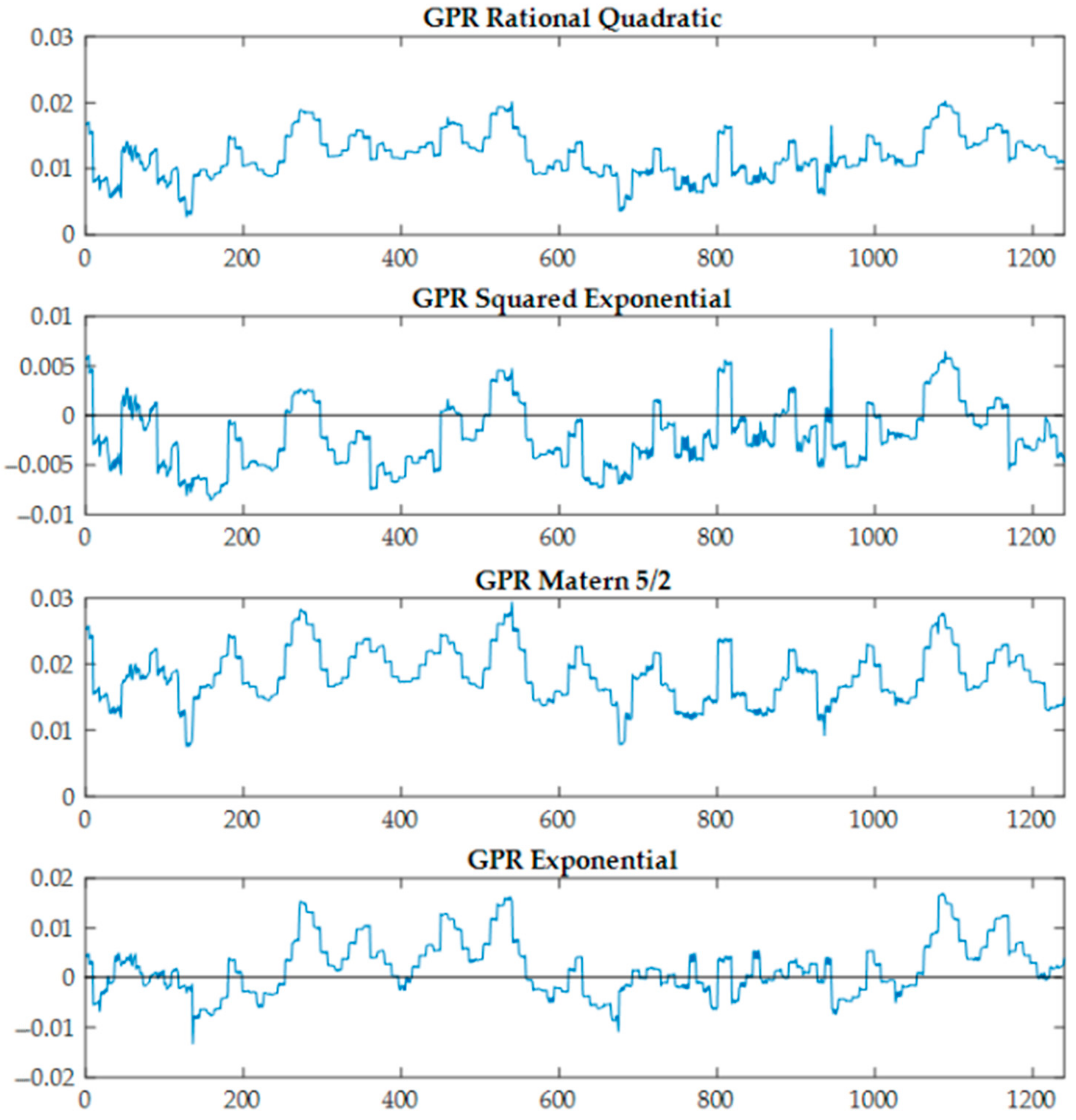
In order to evaluate the model interpolation capability, this work used a new and independent dataset. A new PCA has been fabricated and tested for this purpose. This new PCA has an architecture of three lines, four columns, and one board, and a configuration of 1D: IPOS, 2D: IPOS, 3D: NC. It performed an experimental campaign of 1240 measures in 139 different operating points with nine repetitions for each point. To test the performance of the kernels, the exact same values of operating points applied to the converter during its empirical tests are used as input data in the models. Their predictions are compared with the real efficiency measured during the experiment. The errors that each model presented are presented in Figure 13. The y-axis units are points of efficiency; e.g., at a given operating point where the efficiency was 0.925 and the prediction was 0.935, the efficiency error equals 0.01.

As presented in Figure 13, the SE kernel shows an outstanding performance, predicting all 139 operating points with less than 0.01 point of efficiency (1%) from the actual experimental measures. The EX also presents a decent accuracy. However, the M52 and RQ kernels overvalue the efficiency in all predictions.

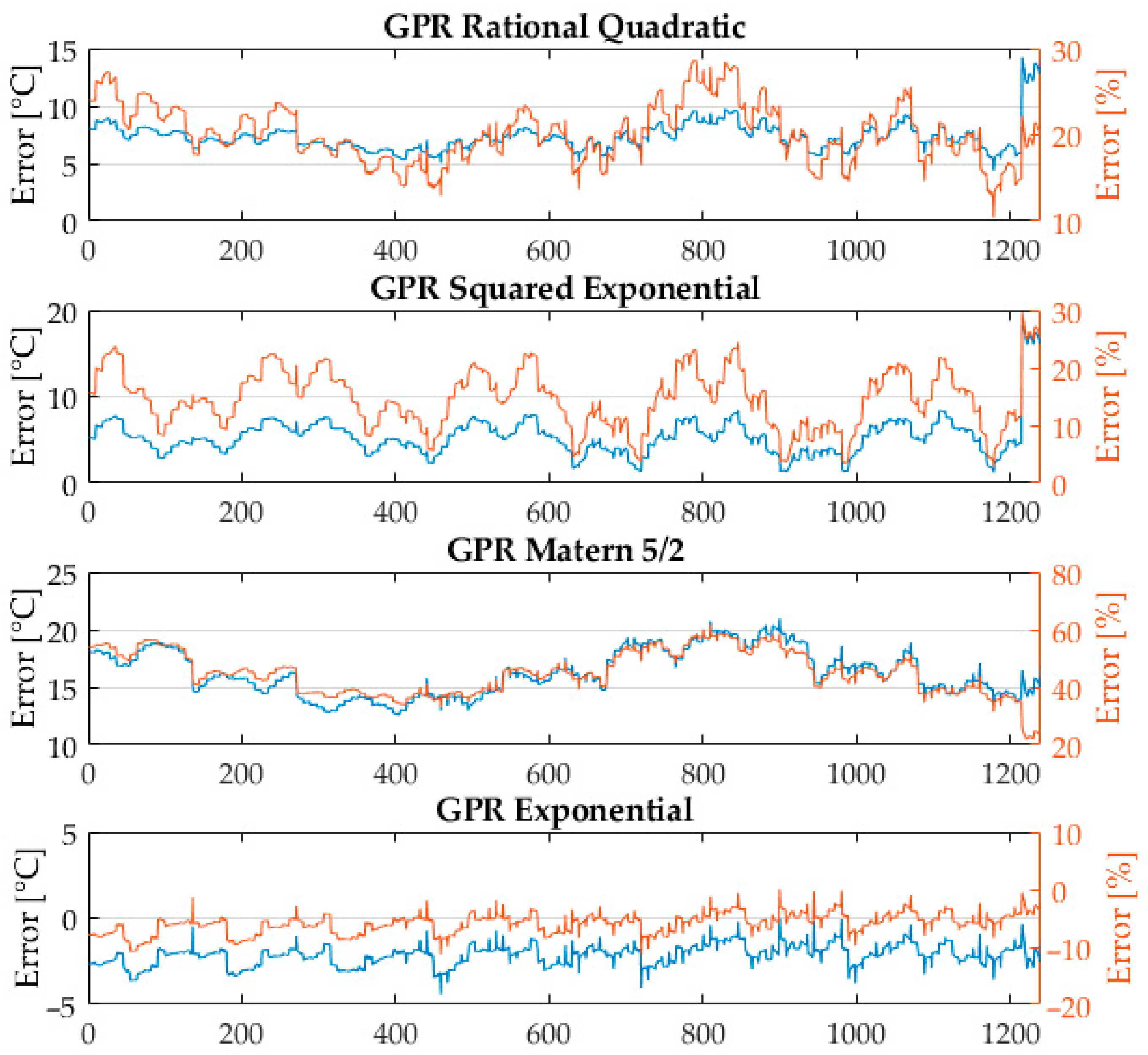
The same comparison was performed with the GPR model focused on predicting the operating temperature of the PCA as a function of all 11 input variables. The same four kernels used for the efficiency model were used to train the temperature GPR model. Similarly, the same independent dataset from the new PCA was used for the final validation. The errors of the temperature predicted by the model to the actual temperatures of the PCA are presented in Figure 14.

The next section shows how virtual prototyping can be carried out based on these models and their accuracy. A brief discussion on the limits of the model and their needs in terms of data is also proposed.

6. Virtual Prototyping and ADFM Discussion

In order to demonstrate how the PCA concept works, this section presents a practical example of the design process of a converter. The specifications of the converter are presented in

Table 5. Specifications of a DC-DC converter for a battery charging application.

Variable	Value
Input Voltage (Battery Side)	32 V to 40 V
Output Current	8 ADC max
Isolation	1.5 kV
Maximum Dimensions (Width × Length × Height)	10 cm × 30 cm × 10 cm
Minimum Efficiency at Nominal Power	91%
Maximum Weight	1 kg

. Its specifications correspond to those of a DC-DC isolated converter for charging and discharging a LiFePO₄ 36 V battery stack from a 120 V DC bus.

Using the specifications presented in Table 5 as input into the ADFM algorithm, the algorithm then selects the technology platform, which is the most adequate to fulfill the required specifications. During this work, the only TP available was the one presented in Section 2. Then, the algorithm performs calculations to define how many CSCs are required and in which configuration they must be in order to fulfill the required specifications. For the sake of brevity, this work does not present details on the algorithm calculations. However, its main mechanism is to find out how many CSCs must be connected in series to achieve the desired voltage and in parallel to achieve the desired current. All possible solutions found by the algorithm are presented in

Table 6. List of PCAs that are able to perform the power conversion described in Table 3.

No.	Architecture	No. of CSCs	Configuration	Max Power [W]	Max Input Voltage [V]	Max Output Voltage [V]	Max Output Current [A]	CPR [%]	Length [mm]	Width [mm]	Height [mm]	Weight [mm]
1	2 × 6 × 1	12	PS-SP-0	1200	40	120	10	100	94	144	13	420
2	1 × 6 × 2	12	PS-0-SP	1200	40	120	10	100	47	144	26	420
3	2 × 3 × 2	12	PS-PS-SP	1200	40	120	10	100	94	72	26	480
4	2 × 3 × 2	12	SP-PS-PS	1200	40	120	10	100	94	72	26	480
5	2 × 7 × 1	14	PS-SP-0	1400	40	140	10	85.7	94	168	13	480
6	1 × 7 × 2	14	PS-0-SP	1400	40	140	10	85.7	47	168	26	480
7	2 × 4 × 2	16	PS-PS-SP	1600	40	160	10	75	94	96	26	600
8	4 × 2 × 2	16	SP-PS-PS	1600	40	160	10	75	188	48	26	720

.

The architectures in which the CSCs are placed are presented in Table 4 with the code (number of lines × number of columns × number of boards). The configuration indicates the type of connections in which the CSCs are connected (SP for input series output parallel and PS for input parallel output series). In some solutions, the input and output voltage maximum values are higher than the required specifications, but they are able to work at the desired voltage. The table also presents the CSC Power Ratio (CPR), which represents the ratio (nominal power/max power) in which the CSCs will work.

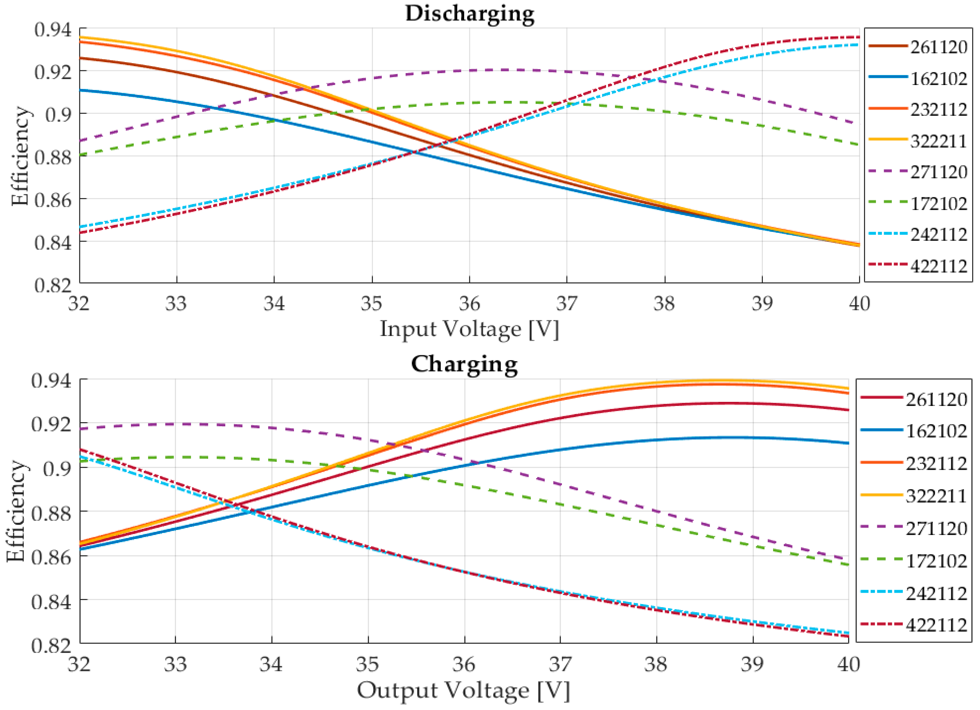
Based on the models developed in Section 5, the performance of all the solutions presented in Table 4 can be compared in detail. The efficiency of each PCA is presented in Figure 15. The plots present the charging and discharging process of the battery for a constant DC bus voltage of 120 V. When charging the battery, the PCA operates in buck mode (from 120 V to 36 V), and while discharging the PCA, it operates in boost mode (from 36 V to 120 V). As the CSCs are DAB converters, it is expected that they present different efficiency values when working in buck or in boost modes. It is imperative to highlight that the ADFM method presents these results automatically without any time-based simulations.

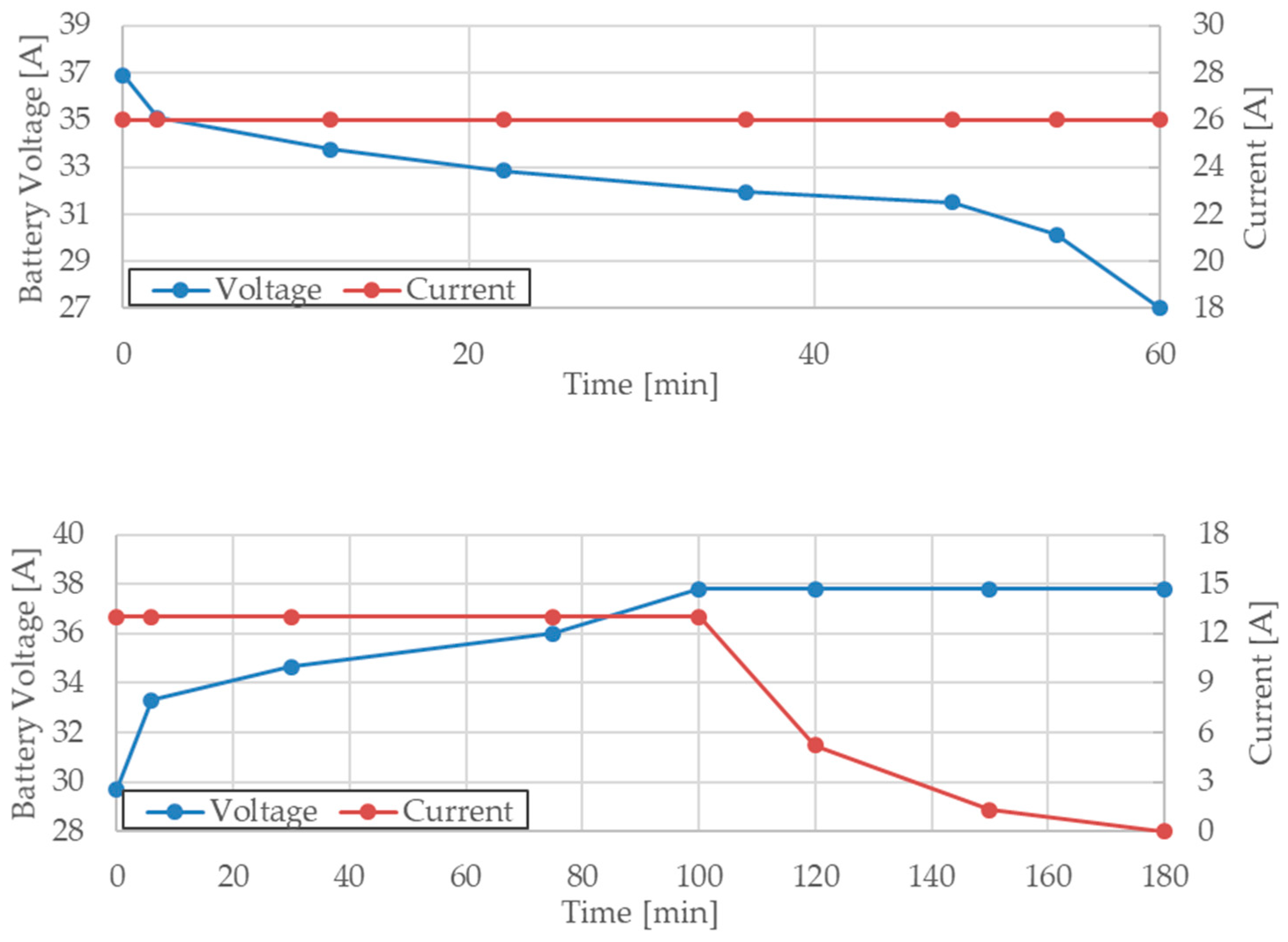
Virtual prototyping can be used to perform a complete analysis of the performance of each PCA for multiple operation points or even a mission profile. Figure 15 shows the mission profile set to charge a specific type of battery. The battery cells studied in the example are the model LIR18650 from the company EEMB [31]. It is possible to identify in the battery datasheet the charge and discharge profiles. These data are used to set up the mission profiles for the charge and the discharge sequences. The battery pack is made of five parallel connected groups of nine cells connected in series. Its charge and discharge characteristic are shown in Figure 16.

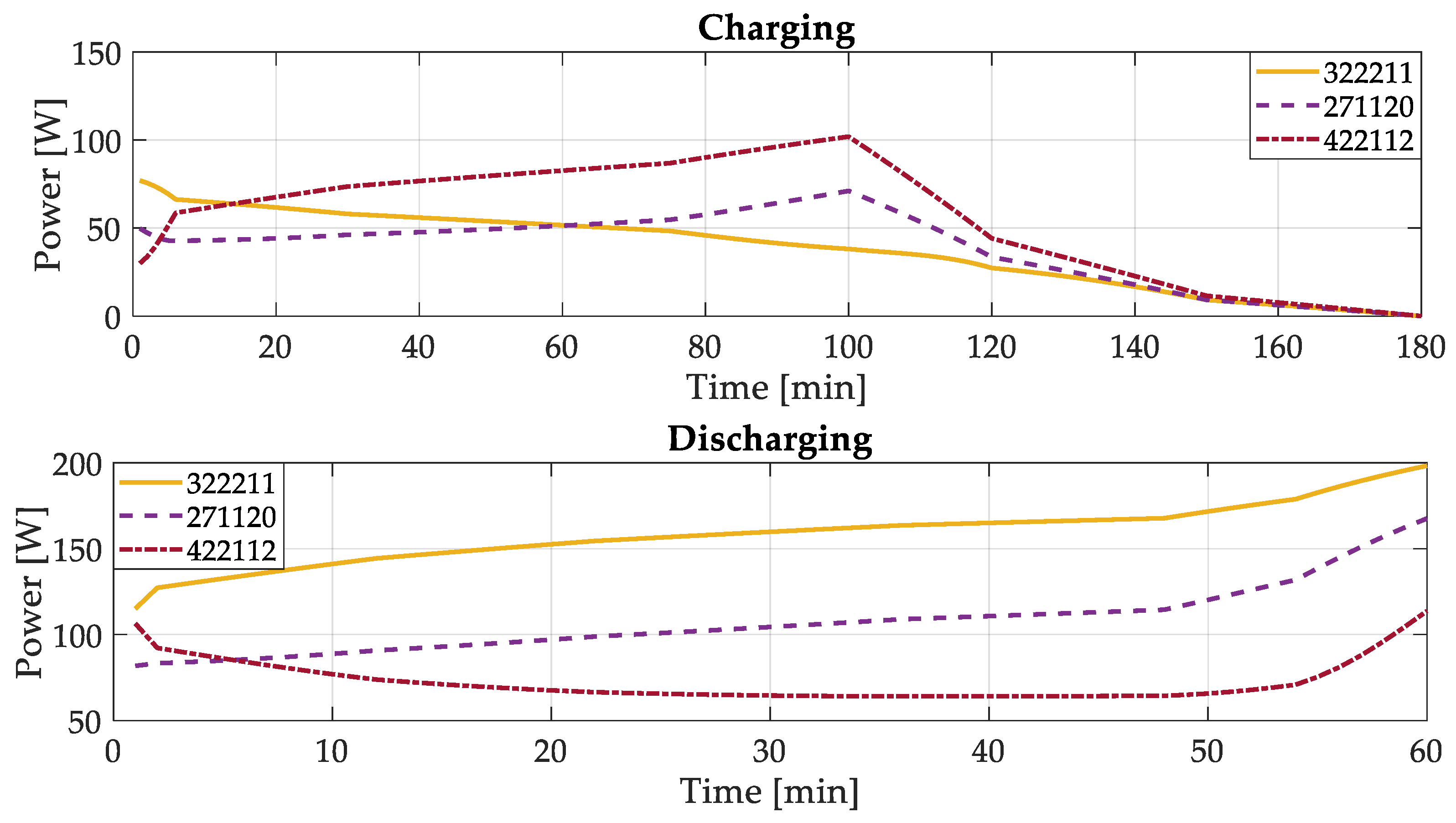
The models created in Section 5 can also be used to predict the performance that each PCA has at each operating point (voltage and current) for an entire mission profile comprising 180 min of the charging sequence and 60 min of the discharging sequence. The three most efficient PCAs presented in Figure 15 were considered for comparison: 322211, 271120, and 422112. Figure 17 shows the instantaneous power loss that each of these solutions presents during the charge and discharge cycles.

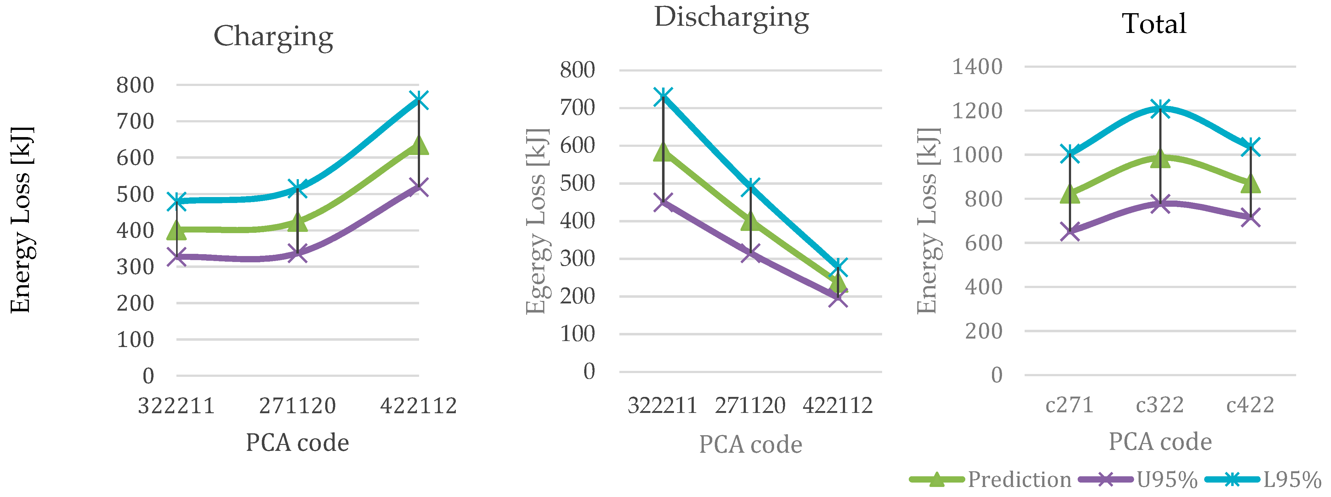
The total energy dissipated during the charging and discharging cycles of each PCA can be calculated by integrating the instantaneous power losses. Figure 18 presents results for each PCA during charge, discharge, and the whole mission profile. The table includes the predictions made using the upper and lower boundaries of the 95% (indicated by U95% and L95%).

It is possible to estimate which PCA presents the best performance for charging and discharging cycles. Figure 18 shows the predicted energy losses for each PCA for charge, discharge, and the total mission profile. It can be seen that the PCA 271120, which presents an average performance in charging and discharging, ends up being the best option for the whole mission profile.

The confidence intervals in Figure 18 show the level of precision of the proposed virtual prototype. By taking them into account, it is much less clear which prototype is should be chosen. This means that more data is required, which is mainly due to the fact that many operation points used in this virtual prototyping are actual extrapolations based on the dataset. For example, the voltage difference (DV) in the dataset is mainly concentrated in −1 to +1.5 V, while in the battery predictions, the DV varied from −5 to 4 V. If the dataset had a wider range of DV, output current, input voltage, etc., the predictions would have been more accurate.

7. Conclusions

Automatic Design for Manufacturing (ADFM) in power electronics revisits the idea of what a power converter is and how to create one. A power converter is created from the interconnection of arrays of Conversion-Standard Cells (CSC), thus creating a Power Converter Array (PCA). CSCs, together with other standard cells, constitute a technology platform (TP). A designer using the ADFM method goes from a set of specifications to the manufacturing files of the PCA through a complete automated process. This process includes virtual prototyping and cross comparing of several PCAs performances. The work was divided in five sections.

Section 2 described what a technology platform is and how it is a fundamental concept in the ADFM methodology. The section also presented the concepts of architecture and configuration, and how Standard Cells are assembled to create Power Converter Arrays.

Section 3 presented a brief comparison of the traditional design flow of power converters with the ADFM methodology. It also described that one fundamental idea behind the ADFM is the use of statistical models to predict the performance of any PCA built from a given technology platform. The creation of these models was explained in the two following sections.

As several electrical and thermal parameters must be studied with several PCAs, strategies of design of experiments (DOE) were applied in order to reduce the amount of experiments. Section 4 presented the main ideas behind selecting the minimal quantity of experiments in order to get the maximum amount of information. In practice, this meant choosing which prototypes to build, in order to save resources, and under which conditions input and output variables should be measured, to save time and resources. Several details of the experimental test bench were also presented.

Section 5 discussed statistical modeling techniques, and it selected the Gaussian Process Regression (GPR) to create a model to predict the efficiency and the temperature of PCAs. The section presented a comparison between four kernels, and their performances were tested. Finally, the best kernel for predicting the efficiency and temperature was the squared exponential.

Finally, the last section presented a virtual prototyping application that compares the performance of PCAs in a charge/discharge battery application. The use of this prediction models opens up a field of exploration into the design of PCAs. Since every operating point of any PCA built with a TP that has been previously characterized can be predicted, any user can analyze the performance of PCAs under any mission profile. This opens up a field to explore optimal solutions to very unique converter specifications and might inspire advances in the field of automated design in power electronics.

The ADFM is an alternative approach to achieve a more automatic design process of power electronic converters. Interesting results were presented in this work; however, there are still many issues about this method to be investigated, such as the following:

Cost: How does the price of a PCA compare to a converter designed by a traditional method? What scale of the mass manufacture of CSCs could represent a significant price reduction for PCAs?

Reliability: A PCA contains several times more components than traditional converters. However, thanks to the multicell approach, it is possible to isolate defective cells and increase the overall reliability. There are several techniques of control and monitoring that can be applied to the methodology. In addition, since fewer types of components as well as assembly and implementation technologies are involved in the manufacture process, these could be optimized toward a very high reliability level at the CSC level, allowing the creation of very reliable PCAs.

EMI and thermal management: Thanks to the usage of standardized elements, it might be possible to predict conducted and radiated emissions of PCAs as well as optimized thermal management conditions. In this case, the automatic design of filters and thermal needs could be achieved.

The overall approach is opening a new design and manufacturing paradigm in power electronics where the standardization of conversion blocs could shift the entire field into automated converter synthesis, with PCA converter mass production players operating various technology platforms (TP) on one side and design houses that are fabless on the other side, answering to end users’ needs. Both would be linked by TP design kits, offering a full description of CSC characteristics, design, and implementation rules. Specific design tools could be developed in order to load specifications, with a comprehensive description language. Then, the design environment would be able to synthesis a PCA from the data made available in the design kits from the PCA manufacturer. This projection is very similar to what has been done, a long time ago, in digital design, and more research of ours will follow.