
An Effective Algorithm for MAED Problems with a New Reliability Model at the Microgrid

 ,
,  ,
, 
Abstract
:1. Introduction
2. MAED Optimization Problems
2.1. Objective Functions
2.1.1. Minimizing Operational Cost Considering Reliability Issues
- 1:
- 2:
- n is the index of available generation units and N is the number of available generation units.
- 3:
- k is the index fuel type and K is the number of fuel types.
- 4:
- Pn is the output power of the nth unit and Pn,max and Pn,min are maximum and minimum output power limits of the nth unit, respectively.
- 5:
- is a quadratic generation cost function for fuel type k of the nth unit.
- 6:
- ank, bnk, and cnk are cost function coefficients of the nth unit for fuel type k.
- 7:
- is sinusoidal and the non-smooth fuel cost function due to the VPL effects for fuel type k of the nth unit.
- 8:
- enk and fnk are cost function coefficients of the VPL effects model of the nth unit for fuel type k.
2.1.2. Minimizing Emissions
- 1:
- 2:
- is emission generated by the nth unit for fuel type k.
- 3:
- ank, βnk, and γnk are the emission coefficients of the nth unit for fuel type k.
2.2. Constraints
2.2.1. Area Total Active Power Balance
2.2.2. Generator Output Power Limits
2.2.3. Ramp-Rate Limits
2.2.4. Prohibited Operating Zones (POZ) Due to Physical Operational Limitations
2.2.5. Maximum and Minimum Power Transfer Through Tie-Lines
2.2.6. Spinning Reserve (SR) Requirement in Each Area
2.2.7. Limitation on Power Transfers Considering SR Contribution
3. Phasor Particle Swarm Optimization (PPSO) Technique
3.1. Background of Different Variants of PSO
3.2. Parameter Setting in PPSO
3.3. Flowchart of PPSO
4. Results and Discussion
4.1. Optimization Results
4.1.1. The MAED Problems Optimization Process Using PPSO
4.1.2. Practical MAED Optimization Problems
4.1.3. RCMAEED and RCMAED Problems
4.1.4. Reliability-Oriented MAED
4.2. Discussion
5. Conclusions
Author Contributions
Funding
Institutional Review Board Statement
Informed Consent Statement
Data Availability Statement
Conflicts of Interest
Nomenclature
| Indices: | |
| Load point index | |
| Committed generation units | |
| Input fuel types | |
| Transmission lines | |
| Area’s index | |
| Decision variable’s index | |
| The number of decision variables | |
| The prohibited operating zones (POZ) | |
| / | The available/unavailable generation units |
| Set of all areas which are connected to qth area | |
| Parameters: | |
| The number of committed generating units in the qth area | |
| Standard deviation | |
| The number of POZs in the nth thermal unit power curve | |
| The fuel cost coefficients of nth thermal unit | |
| The fuel cost coefficients of nth thermal unit for kth fuel type | |
| The down ramp rate-limit of nth thermal unit | |
| The up ramp rate-limits of nth thermal unit | |
| The power output of nth thermal unit in the first stage | |
| The minimum power output of nth thermal unit | |
| The maximum power output of nth thermal unit | |
| The minimum power output of nth thermal unit for kth fuel type | |
| The maximum power output of nth thermal unit for kth fuel type | |
| The lower bound for prohibited zone k of nth thermal unit | |
| The upper bound for prohibited zone k of nth thermal unit | |
| System total load demand | |
| The power demand in qth area | |
| The maximum capacity of the tie-line between qth and wth areas | |
| The emission coefficients of nth thermal unit for kth fuel type | |
| The spinning reserve requirement in the qth area | |
| User defined weighting factor for emission cost (in this study: 120) | |
| Penalty coefficient value | |
| Number of initial population | |
| The current position vector of ith particle | |
| The current velocity vector of ith particle | |
| Maximum number of iterations for PSO algorithm | |
| The best personal position vector of ith particle | |
| The global best position vector | |
| The phase angle | |
| The cost of energy not supplied () | |
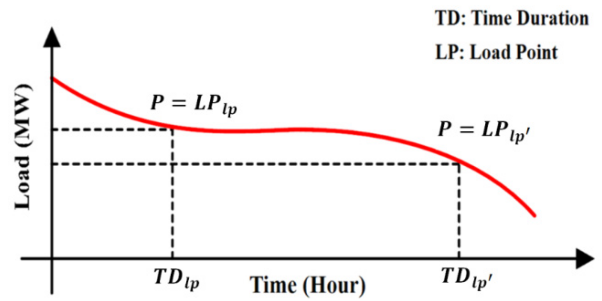
| Expected power not supplied at load point | |
| The time duration of load point | |
| The probability of availability and unavailability of generation | |
| / | The set of available (unavailable) generation units |
| The failure rate of nth generator | |
| The repair rate of nth generator | |
| Mean time to repair nth generator | |
| Mean time to failure of nth generator | |
| Failure time of nth generator | |
| Repair time of nth generator | |
| Unavailability (force outage rate) of nth generator | |
| Functions and Variables: | |
| Objective function | |
| The fuel cost function of nth thermal unit | |
| The power output of nth thermal unit | |
| Cost function associated with jth transmission line | |
| Active power flow through jth transmission line | |
| The power flow from qth area to wth area | |
| The emission function of nth thermal unit | |
| The amount of reserve contributed between qth and wth areas | |
| The reserve provided by all thermal units in the nth area | |
| Abbreviations: | |
| APSO: | Adaptive PSO |
| CEP: | Classical evolutionary programming |
| CENS | Cost of energy not supplied |
| CLPSO: | Comprehensive learning PSO |
| DEC2: | Chaotic DE/2 algorithm |
| DSM: | Direct search method |
| EENS: | Expected energy not supplied |
| ELD: | Economic load dispatch |
| EP: | Evolutionary programming |
| FIPS: | Fully informed particle swarm |
| FPSO: | Frankenstein’s PSO |
| HNN: | Hopfield neural network |
| HS: | Harmony search |
| HSLSO: | Hybridizing sum-local search optimizer |
| LOLP: | Loss of Load Probability |
| MAED: | Multi-area economic dispatch |
| NFP: | Network flow programming |
| POZ: | Prohibited operating zones |
| PPSO: | Phasor particle swarm optimization |
| PS: | Pattern search |
| PSO: | Particle swarm optimization |
| PSO-cf: | Modified PSO by constriction factor |
| PSO-TVAC: | Self-organizing hierarchical particle swarm optimizer with time-varying acceleration coefficients |
| PSO-ω: | Modified PSO by the inertia weight |
| RCMAED: | Reserve constrained multi-area economic dispatch |
| RCMAEED: | Reserve constrained multi-area environmental/economic dispatch |
| SPSO2011: | The improved standard PSO 2011 |
| SR: | Spinning reserve |
| VPL: | Valve-point loading |
References
- Naderipour, A.; Abdul-Malek, Z.; Nowdeh, S.A.; Ramachandaramurthy, V.K.; Kalam, A.; Guerrero, J.M. Optimal allocation for combined heat and power system with respect to maximum allowable capacity for reduced losses and improved voltage profile and reliability of microgrids considering loading condition. Energy 2020, 196, 117124. [Google Scholar] [CrossRef]
- Fu, C.; Zhang, S.; Chao, K.-H. Energy management of a power system for economic load dispatch using the artificial intelligent algorithm. Electronics 2020, 9, 108. [Google Scholar] [CrossRef] [Green Version]
- Fu, B.; Ouyang, C.; Li, C.; Wang, J.; Gul, E. An improved mixed integer linear programming approach based on symmetry diminishing for unit commitment of hybrid power system. Energies 2019, 12, 833. [Google Scholar] [CrossRef] [Green Version]
- Abido, M.A. Multiobjective evolutionary algorithms for electric power dispatch problem. IEEE Trans. Evol. Comput. 2006, 10, 315–329. [Google Scholar] [CrossRef]
- Ren, Y.; Fei, S. The auxiliary problem principle with self-adaptive penalty parameter for multi-area economic dispatch problem. Algorithms 2015, 8, 144–156. [Google Scholar] [CrossRef] [Green Version]
- Nowdeh, S.A.; Nasri, S.; Saftjani, P.B.; Naderipour, A.; Abdul-Malek, Z.; Kamyab, H.; Nowdeh, A.J. Multi-Criteria Optimal Design of Hybrid Clean Energy System with Battery Storage Considering Off- and On-Grid Application. J. Clean. Prod. 2020. [Google Scholar] [CrossRef]
- Abdollahi, E.; Wang, H.; Lahdelma, R. An optimization method for multi-area combined heat and power production with power transmission network. Appl. Energy 2016, 168, 248–256. [Google Scholar] [CrossRef]
- Sharma, M.; Pandit, M.; Srivastava, L. Reserve constrained multi-area economic dispatch employing differential evolution with time-varying mutation. Int. J. Electr. Power Energy Syst. 2011, 33, 753–766. [Google Scholar] [CrossRef]
- Yu, J.; Kim, C.-H.; Wadood, A.; Khurshiad, T.; Rhee, S.-B. A novel multi-population based chaotic JAYA algorithm with application in solving economic load dispatch problems. Energies 2018, 11, 1946. [Google Scholar] [CrossRef] [Green Version]
- Ghasemi, M.; Aghaei, J.; Akbari, E.; Ghavidel, S.; Li, L. A differential evolution particle swarm optimizer for various types of multi-area economic dispatch problems. Energy 2016, 107, 182–195. [Google Scholar] [CrossRef] [Green Version]
- Jadoun, V.K.; Gupta, N.; Niazi, K.R.; Swarnkar, A. Modulated particle swarm optimization for economic emission dispatch. Int. J. Electr. Power Energy Syst. 2015, 73, 80–88. [Google Scholar] [CrossRef]
- Ghasemi, A. A fuzzified multi objective interactive honey bee mating optimization for environmental/economic power dispatch with valve point effect. Int. J. Electr. Power Energy Syst. 2013, 49, 308–321. [Google Scholar] [CrossRef]
- Dubey, H.M.; Pandit, M.; Tyagi, N.; Panigrahi, B.K. Wind integrated multi area economic dispatch using backtracking search algorithm. In Proceedings of the 2016 IEEE 6th International Conference on Power Systems (ICPS), New Delhi, India, 4–6 March 2016; pp. 1–6. [Google Scholar]
- Mokarram, M.J.; Niknam, T.; Aghaei, J.; Shafie-khah, M.; Catalao, J.P.S. Hybrid optimization algorithm to solve the nonconvex multiarea economic dispatch problem. IEEE Syst. J. 2019, 13, 3400–3409. [Google Scholar] [CrossRef]
- Vijayaraj, S.; Santhi, R.K. Multi-Area economic dispatch using flower pollination algorithm. In Proceedings of the 2016 International Conference on Electrical, Electronics, and Optimization Techniques (ICEEOT), Chennai, India, 3–5 March 2016; pp. 4355–4360. [Google Scholar]
- Azizipanah-Abarghooee, R.; Dehghanian, P.; Terzija, V. Practical multi-area bi-objective environmental economic dispatch equipped with a hybrid gradient search method and improved Jaya algorithm. IET Gener. Transm. Distrib. 2016, 10, 3580–3596. [Google Scholar] [CrossRef] [Green Version]
- Lin, J.; Wang, Z.-J. Multi-Area economic dispatch using an improved stochastic fractal search algorithm. Energy 2019, 166, 47–58. [Google Scholar] [CrossRef]
- Ghasemi, M.; Davoudkhani, I.F.; Akbari, E.; Rahimnejad, A.; Ghavidel, S.; Li, L. A novel and effective optimization algorithm for global optimization and its engineering applications: Turbulent Flow of Water-based Optimization (TFWO). Eng. Appl. Artif. Intell. 2020, 92, 103666. [Google Scholar] [CrossRef]
- Nguyen, K.P.; Dinh, N.D.; Fujita, G. Multi-Area economic dispatch using Hybrid Cuckoo search algorithm. In Proceedings of the 2015 50th International Universities Power Engineering Conference (UPEC), Stoke on Trent, UK, 1–4 September 2015; pp. 1–6. [Google Scholar]
- Basu, M. Artificial bee colony optimization for multi-area economic dispatch. Int. J. Electr. Power Energy Syst. 2013, 49, 181–187. [Google Scholar] [CrossRef]
- Chen, C.-L.; Chen, Z.-Y.; Lee, T.-Y. Multi-Area economic generation and reserve dispatch considering large-scale integration of wind power. Int. J. Electr. Power Energy Syst. 2014, 55, 171–178. [Google Scholar] [CrossRef]
- Secui, D.C. The chaotic global best artificial bee colony algorithm for the multi-area economic/emission dispatch. Energy 2015, 93, 2518–2545. [Google Scholar] [CrossRef]
- Ghasemi, M.; Ghavidel, S.; Aghaei, J.; Akbari, E.; Li, L. CFA optimizer: A new and powerful algorithm inspired by Franklin’s and Coulomb’s laws theory for solving the economic load dispatch problems. Int. Trans. Electr. Energy Syst. 2018, 28, e2536. [Google Scholar] [CrossRef] [Green Version]
- Shi, Y.; Eberhart, R. A modified particle swarm optimizer. In Proceedings of the 1998 IEEE International Conference on Evolutionary Computation Proceedings, IEEE World Congress on Computational Intelligence (Cat. No. 98TH8360), Anchorage, AK, USA, 4–9 May 1998; pp. 69–73. [Google Scholar]
- Laganà, D.; Mastroianni, C.; Meo, M.; Renga, D. Reducing the operational cost of cloud data centers through renewable energy. Algorithms 2018, 11, 145. [Google Scholar] [CrossRef] [Green Version]
- Chaiyabut, N.; Damrongkulkumjorn, P. Optimal spinning reserve for wind power uncertainty by unit commitment with EENS constraint. In Proceedings of the ISGT, Washington, DC, USA, 19–22 February 2014; pp. 1–5. [Google Scholar]
- Khokhar, S.; Zin, A.A.M.; Mokhtar, A.S.; Bhayo, M.A.; Naderipour, A. Automatic classification of single and hybrid power quality disturbances using Wavelet Transform and Modular Probabilistic Neural Network. In Proceedings of the 2015 IEEE Conference on Energy Conversion, CENCON 2015, Johor Bahru, Malaysia, 19–20 October 2015; pp. 457–462. [Google Scholar]
- Ajmal, A.M.; Ramachandaramurthy, V.K.; Naderipour, A.; Ekanayake, J.B. Comparative analysis of two-step GA-based PV array reconfiguration technique and other reconfiguration techniques. Energy Convers. Manag. 2021, 230, 113806. [Google Scholar] [CrossRef]
- Naderipour, A.; Abdul-Malek, Z.; Nowdeh, S.A.; Kamyab, H.; Ramtin, A.R.; Shahrokhi, S.; Klemeš, J.J. Comparative evaluation of hybrid photovoltaic, wind, tidal and fuel cell clean system design for different regions with remote application considering cost. J. Clean. Prod. 2020. [Google Scholar] [CrossRef]
- Naderipour, A.; Abdul-Malek, Z.; Nowdeh, S.A.; Gandoman, F.H.; Moghaddam, M.J.H. A multi-objective optimization problem for optimal site selection of wind turbines for reduce losses and improve voltage profile of distribution grids. Energies 2019, 12, 2621. [Google Scholar] [CrossRef] [Green Version]
- Naderipour, A.; Abdul-Malek, Z.; Vahid, M.Z.; Seifabad, Z.M.; Hajivand, M.; Arabi-Nowdeh, S. Optimal, reliable and cost-effective framework of photovoltaic-wind-battery energy system design considering outage concept using grey wolf optimizer algorithm—Case study for iran. IEEE Access 2019, 7, 182611–182623. [Google Scholar] [CrossRef]
- Lasemi, M.A.; Assili, M.; Baghayipour, M. Modification of multi-area economic dispatch with multiple fuel options, considering the fuelling limitations. IET Gener. Transm. Distrib. 2014, 8, 1098–1106. [Google Scholar] [CrossRef]
- Roy, P.K.; Hazra, S. Economic emission dispatch for wind–fossil-fuel-based power system using chemical reaction optimisation. Int. Trans. Electr. Energy Syst. 2015, 25, 3248–3274. [Google Scholar] [CrossRef]
- Niknam, T. A new fuzzy adaptive hybrid particle swarm optimization algorithm for non-linear, non-smooth and non-convex economic dispatch problem. Appl. Energy 2010, 87, 327–339. [Google Scholar] [CrossRef]
- Ganjefar, S.; Tofighi, M. Dynamic eNconomic dispatch solution using an improved genetic algorithm with non-stationary penalty functions. Eur. Trans. Electr. Power 2011, 21, 1480–1492. [Google Scholar] [CrossRef]
- Wang, L.; Singh, C. Reserve-Constrained multiarea environmental/economic dispatch based on particle swarm optimization with local search. Eng. Appl. Artif. Intell. 2009, 22, 298–307. [Google Scholar] [CrossRef]
- Jensi, R.; Jiji, G.W. An enhanced particle swarm optimization with levy flight for global optimization. Appl. Soft Comput. 2016, 43, 248–261. [Google Scholar] [CrossRef]
- Clerc, M.; Kennedy, J. The particle swarm-explosion, stability, and convergence in a multidimensional complex space. IEEE Trans. Evol. Comput. 2002, 6, 58–73. [Google Scholar] [CrossRef] [Green Version]
- Ratnaweera, A.; Halgamuge, S.K.; Watson, H.C. Self-Organizing hierarchical particle swarm optimizer with time-varying acceleration coefficients. IEEE Trans. Evol. Comput. 2004, 8, 240–255. [Google Scholar] [CrossRef]
- Ghasemi, M.; Akbari, E.; Rahimnejad, A.; Razavi, S.E.; Ghavidel, S.; Li, L. Phasor particle swarm optimization: A simple and efficient variant of PSO. Soft Comput. 2019, 23, 9701–9718. [Google Scholar] [CrossRef]
- Zhan, Z.-H.; Zhang, J.; Li, Y.; Chung, H.S.-H. Adaptive particle swarm optimization. IEEE Trans. Syst. Man Cybern. Part 2009, 39, 1362–1381. [Google Scholar] [CrossRef] [PubMed] [Green Version]
- Liang, J.J.; Qin, A.K.; Suganthan, P.N.; Baskar, S. Comprehensive learning particle swarm optimizer for global optimization of multimodal functions. IEEE Trans. Evol. Comput. 2006, 10, 281–295. [Google Scholar] [CrossRef]
- Zambrano-Bigiarini, M.; Clerc, M.; Rojas, R. Standard particle swarm optimisation 2011 at cec-2013: A baseline for future pso improvements. In Proceedings of the 2013 IEEE Congress on Evolutionary Computation, Cancun, Mexico, 20–23 June 2013; pp. 2337–2344. [Google Scholar]
- Mendes, R.; Kennedy, J.; Neves, J. The fully informed particle swarm: Simpler, maybe better. IEEE Trans. Evol. Comput. 2004, 8, 204–210. [Google Scholar] [CrossRef]
- De Oca, M.A.M.; Stutzle, T.; Birattari, M.; Dorigo, M. Frankenstein’s PSO: A composite particle swarm optimization algorithm. IEEE Trans. Evol. Comput. 2009, 13, 1120–1132. [Google Scholar] [CrossRef]
- Yalcinoz, T.; Short, M.J. Neural networks approach for solving economic dispatch problem with transmission capacity constraints. IEEE Trans. Power Syst. 1998, 13, 307–313. [Google Scholar] [CrossRef]
- Chen, C.-L.; Chen, N. Direct search method for solving economic dispatch problem considering transmission capacity constraints. IEEE Trans. Power Syst. 2001, 16, 764–769. [Google Scholar] [CrossRef]
- Fesanghary, M.; Ardehali, M.M. A novel meta-heuristic optimization methodology for solving various types of economic dispatch problem. Energy 2009, 34, 757–766. [Google Scholar] [CrossRef]
- Pandit, M.; Srivastava, L.; Pal, K. Static/Dynamic optimal dispatch of energy and reserve using recurrent differential evolution. IET Gener. Transm. Distrib. 2013, 7, 1401–1414. [Google Scholar] [CrossRef]
- Soroudi, A.; Rabiee, A. Optimal multi-area generation schedule considering renewable resources mix: A real-time approach. IET Gener. Transm. Distrib. 2013, 7, 1011–1026. [Google Scholar] [CrossRef] [Green Version]
- Jayabarathi, V.; Ramachandran, T.G.S. Evolutionary programming-based multiarea economic dispatch with tie line constraints. Electr. Mach. Power Syst. 2000, 28, 1165–1176. [Google Scholar] [CrossRef]
- Zhu, J.; Momoh, J.A. Multi-Area power systems economic dispatch using nonlinear convex network flow programming. Electr. Power Syst. Res. 2001, 59, 13–20. [Google Scholar] [CrossRef]
- Al-Sumait, J.S.; Sykulski, J.K.; Al-Othman, A.K. Solution of different types of economic load dispatch problems using a pattern search method. Electr. Power Compon. Syst. 2008, 36, 250–265. [Google Scholar] [CrossRef]


| Method | P1 (MW) | P2 (MW) | P3 (MW) | P4 (MW) | T12 (MW) | Cost ($/H) | |
|---|---|---|---|---|---|---|---|
| HNN [46] | - | - | - | - | - | - | 10,605 |
| DSM [47] | - | - | - | - | - | - | 10,605 |
| PSO-TVAC [8] | 444.8047 | 139.1953 | 211.0609 | 324.9391 | −200 | 1120 | 10,604.68 |
| PPSO | 445.1223 | 138.8778 | 212.0426 | 323.9573 | −199.9999 | 1120 | 10,604.67 |
| APSO | 445.3207 | 138.6794 | 212.2054 | 323.7945 | −199.9999 | 1120 | 10,604.67 |
| CLPSO | 445.1213 | 138.8788 | 212.0413 | 323.9586 | −199.9999 | 1120 | 10,604.67 |
| SPSO2011 | 445.1223 | 138.8778 | 212.0426 | 323.9573 | −199.9999 | 1120 | 10,604.67 |
| FPSO | 445.0654 | 138.9347 | 211.9258 | 324.0741 | −199.9999 | 1120 | 10,604.67 |
| FIPS | 445.2274 | 138.7727 | 211.9977 | 324.0022 | −199.9999 | 1120 | 10,604.67 |
| Area No. | PSO [10] | HHS [48] | NFP [52] | CEP [51] | PS [53] | HSLSO [10] | PPSO | |
|---|---|---|---|---|---|---|---|---|
| 1 (400 MW) | P1 (MW) | 150 | 150 | 150 | 150 | 150 | 150 | 150 |
| P2 (MW) | 100 | 100 | 100 | 100 | 100 | 100 | 100 | |
| P3 (MW) | 67.366 | 66.86 | 66.97 | 68.826 | 66.971 | 67.3848 | 67.31016 | |
| P4 (MW) | 100 | 100 | 100 | 99.985 | 100 | 100 | 100 | |
| 2 (200 MW) | P5 (MW) | 56.613 | 57.04 | 56.97 | 56.373 | 56.9718 | 57.0625 | 57.07953 |
| P6 (MW) | 95.474 | 96.22 | 96.25 | 93.519 | 96.2518 | 96.1749 | 96.34877 | |
| P7 (MW) | 41.617 | 41.74 | 41.87 | 42.546 | 41.8718 | 41.8472 | 41.86785 | |
| P8 (MW) | 72.356 | 72.5 | 72.52 | 72.647 | 72.5218 | 72.4505 | 72.53403 | |
| 3 (350 MW) | P9 (MW) | 50 | 50 | 50 | 50 | 50.002 | 50 | 50 |
| P10 (MW) | 35.973 | 36.24 | 36.27 | 36.399 | 36.272 | 36.319 | 36.28298 | |
| P11 (MW) | 38.21 | 38.39 | 38.49 | 38.323 | 38.492 | 38.5911 | 38.50812 | |
| P12 (MW) | 37.162 | 37.2 | 37.32 | 36.903 | 37.322 | 37.3719 | 37.26609 | |
| 4 (300 MW) | P13 (MW) | 150 | 150 | 150 | 150 | 150 | 150 | 150 |
| P14 (MW) | 100 | 100 | 100 | 100 | 100 | 100 | 100 | |
| P15 (MW) | 57.83 | 56.9 | 57.05 | 56.648 | 57.051 | 56.9272 | 56.9218 | |
| P16 (MW) | 97.349 | 96.2 | 96.27 | 95.826 | 96.271 | 95.8709 | 95.88068 | |
| Tie-line power flow | T12 (MW) | 0 | 0 | 0 | −0.018 | 0 | 0 | 0 |
| T13 (MW) | 22.588 | 16.86 | 18.18 | 19.587 | 18.181 | 17.4643 | 17.42629 | |
| T14 (MW) | −5.176 | 0 | −1.21 | −0.758 | −1.21 | −0.0795 | −0.116132 | |
| T23 (MW) | 66.064 | 70.61 | 69.73 | 68.861 | 69.73 | 70.2537 | 70.51652 | |
| T24 (MW) | −0.004 | −3.11 | −2.11 | −1.789 | −2.111 | −2.7186 | −2.686341 | |
| T34 (MW) | −100 | −100 | −100 | −99.927 | −100 | −100 | −100 | |
| 1249.95 | 1249.29 | 1249.98 | 1247.995 | 1249.998 | 1250 | 1250 | ||
| Cost ($/H) | 7336.93 | 7329.85 | 7337 | 7337.75 | 7336.98 | 7337.03 | 7337.026 | |
| Area 1 (PD = 7500 MW) | Area 2 (PD = 3000 MW) | ||||||
|---|---|---|---|---|---|---|---|
| Output (MW) | DEC2 [8] | HSLSO [10] | PPSO | Output (MW) | DEC2 [8] | HSLSO [10] | PPSO |
| P1 | 112.8292 | 110.8012 | 110.8012 | P21 (MW) | 343.7598 | 523.2792 | 523.2794 |
| P2 | 114 | 113.9997 | 113.9998 | P22 (MW) | 433.5196 | 523.2791 | 523.2794 |
| P3 | 97.3999 | 120 | 120 | P23 (MW) | 523.2794 | 523.2794 | 523.2795 |
| P4 | 179.7331 | 179.7331 | 179.7332 | P24 (MW) | 550 | 523.2794 | 523.2794 |
| P5 | 97 | 95.551 | 95.5504 | P25 (MW) | 550 | 523.2795 | 523.2793 |
| P6 | 68.0001 | 140 | 140 | P26 (MW) | 254 | 254 | 254 |
| P7 | 300 | 300 | 300 | P27 (MW) | 10 | 10.0001 | 10 |
| P8 | 284.5997 | 284.5997 | 284.5997 | P28 (MW) | 10.0001 | 10 | 10 |
| P9 | 284.5997 | 284.5997 | 284.5997 | P29 (MW) | 10 | 10 | 10 |
| P10 | 130 | 270 | 270 | P30 (MW) | 47 | 87.7997 | 87.7997 |
| P11 | 360 | 94 | 94.0002 | P31 (MW) | 159.7331 | 188.5959 | 188.5954 |
| P12 | 94.0001 | 300 | 300 | P32 (MW) | 190 | 159.7331 | 159.7331 |
| P13 | 304.5196 | 304.5195 | 304.5195 | P33 (MW) | 163.7269 | 159.733 | 159.7331 |
| P14 | 500 | 394.2797 | 394.2793 | P34 (MW) | 164.7998 | 164.8002 | 164.8 |
| P15 | 484.0392 | 484.0395 | 484.0395 | P35 (MW) | 200 | 164.7998 | 164.7998 |
| P16 | 500 | 484.0391 | 484.0391 | P36 (MW) | 164.7998 | 164.7998 | 164.7992 |
| P17 | 489.2794 | 489.2794 | 489.2797 | P37 (MW) | 110 | 89.1143 | 89.1143 |
| P18 | 500 | 489.2796 | 489.2794 | P38 (MW) | 57.0571 | 89.114 | 89.1142 |
| P19 | 550 | 549.9998 | 549.9998 | P39 (MW) | 25 | 89.1134 | 89.1142 |
| P20 | 550 | 511.2791 | 511.2794 | P40 (MW) | 511.2794 | 242.0001 | 242 |
| T12 (MW) | −1500 | −1500 | −1500 | Cost ($/H) | 127,344.9 | 125,100.3 | 125,100.2 |
| Test System | Index | FIPS | FPSO | SPSO2011 | CLPSO | APSO | PPSO |
|---|---|---|---|---|---|---|---|
| small-scale system | Best | 10,604.6742 | 10,604.67 | 10,604.6741 | 10,604.67 | 10,604.67 | 10,604.67 |
| Mean | 10,605.3272 | 10,604.92 | 10,604.8543 | 10,604.68 | 10,604.73 | 10,604.67 | |
| Std | 1.5275 | 1.1547 | 0.5774 | 0.7022 | 0.4407 | 5.75 × 10⁻⁵ | |
| Mean time (s) | 4.56 | 4.78 | 4 | 3.16 | 6.82 | 2.93 | |
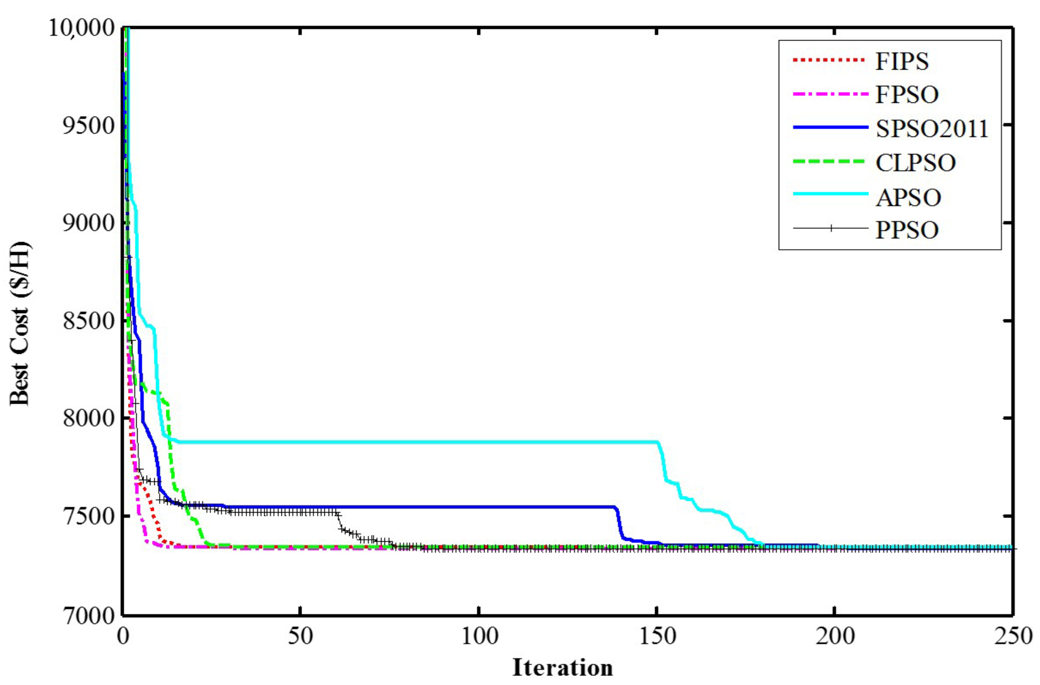
| medium-scale system | Best | 7341.7942 | 7340.455 | 7340.2795 | 7344.357 | 7341.714 | 7337.026 |
| Mean | 7559.7788 | 7487.087 | 7637.4443 | 7486.892 | 7605.919 | 7338.115 | |
| Std | 74.2674 | 61.8126 | 71.271 | 84.3494 | 53.07 | 0.629 | |
| Mean time (s) | 20.95 | 20.67 | 19.19 | 18.31 | 25.57 | 17.84 | |
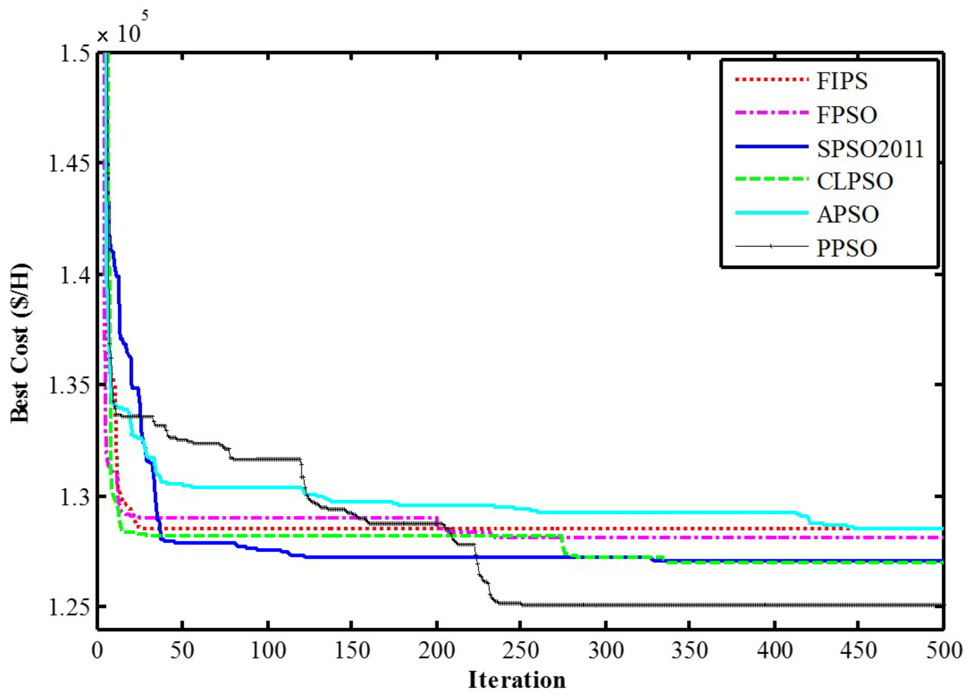
| large-scale system | Best | 128,554.2844 | 128,128.2 | 127,085.5386 | 127,008.9 | 128,514 | 125,100.2 |
| Mean | 130,615.4572 | 129,486 | 129,414.4588 | 128,315.4 | 129,495.4 | 125,263.2 | |
| Std | 1.19 × 10³ | 1.02 × 10³ | 9.84 × 10² | 2.16 × 10² | 6.93 × 10² | 85.3092 | |
| Mean time (s) | 54.74 | 55.85 | 48.51 | 48.35 | 75.3 | 47.88 |
| Output (MW) | FIPS | FPSO | SPSO2011 | CLPSO | APSO | PPSO |
|---|---|---|---|---|---|---|
| P1 | 8.5605 | 8.7146 | 8.1347 | 9.9192 | 8.468 | 11.1868 |
| P2 | 9.9835 | 10 | 8.011 | 7.259 | 8.011 | 9.9596 |
| P3 | 11.26 | 12.3534 | 13 | 8.7913 | 12.7035 | 6.6997 |
| P4 | 0.2616 | 0.05 | 1.9639 | 4.8491 | 1.605 | 2.982 |
| P5 | 18.807 | 22.1526 | 19.5629 | 23.6046 | 20.1371 | 22.8244 |
| P6 | 11.261 | 9.4047 | 10.9592 | 9.2998 | 8.8157 | 8.8553 |
| P7 | 6.1084 | 3.833 | 2.1895 | 3.9163 | 4.7532 | 3.9286 |
| P8 | 15.2128 | 17.2551 | 17.925 | 16.3556 | 17.925 | 17.2481 |
| P9 | 4.6622 | 6.0147 | 2.9329 | 6.1264 | 22.0733 | 5.8222 |
| P10 | 10.5192 | 6.1858 | 8.5093 | 0.05 | 5.3173 | 0.1993 |
| P11 | 20.4782 | 9.1548 | 23.2033 | 9.8982 | 7.4855 | 9.6888 |
| P12 | 4.0058 | 17.2236 | 5.1026 | 22.3468 | 5.1026 | 22.8171 |
| P13 | 11 | 8.1669 | 9.8282 | 9.1629 | 9.8282 | 8.0614 |
| P14 | 20 | 19.7135 | 17.7366 | 19.9614 | 17.7366 | 19.8021 |
| P15 | 26.8153 | 28.7234 | 30 | 28.1791 | 30 | 29.8714 |
| P16 | 0.1384 | 1.2864 | 0.05 | 0.0869 | 0.05 | 0.0534 |
| P17 | 0.1275 | 0.9452 | 0.5512 | 0.1 | 0.5512 | 0.486 |
| P18 | 0.3016 | 0.2525 | 0.2146 | 0.2701 | 0.1433 | 0.204 |
| P19 | 0.1 | 0.18 | 0.3539 | 0.3648 | 0.143 | 0.138 |
| P20 | 0.1 | 1.4402 | 0.1105 | 1.4421 | 0.1105 | 1.4566 |
| P21 | 1.1012 | 1.8441 | 1.1357 | 1.84 | 1.8756 | 1.8858 |
| P22 | 0.1 | 0.1 | 0.2364 | 0.1034 | 0.2364 | 0.188 |
| RC12 | 1.6842 | 2.2985 | 0.3671 | 0.6544 | 2.5336 | 1.5336 |
| RC13 | 0.2249 | 0.1 | 0.1 | 0.8206 | 0.1 | 0.5945 |
| RC14 | 1.8788 | 1.3163 | 2.1507 | 0.2931 | 1.05 | 0.1674 |
| RC23 | 0.4049 | 0.2073 | 0.1 | 0.1 | 1.0058 | 0.1001 |
| RC24 | 0.1645 | 2.4179 | 1.0183 | 1.6712 | 1.0183 | 2.1473 |
| RC34 | 0.4582 | 0.1 | 0.602 | 0.2867 | 0.602 | 0.3759 |
| Reserve area 1 | 18.9344 | 17.882 | 17.8904 | 18.1814 | 18.2125 | 18.1719 |
| Reserve area 2 | 23.6108 | 22.3546 | 24.3634 | 21.8237 | 23.369 | 22.1436 |
| Reserve area 3 | 80.3346 | 81.4211 | 80.2519 | 81.5786 | 80.0213 | 81.4726 |
| Reserve area 4 | 33.0463 | 33.1098 | 33.3852 | 33.6097 | 33.3852 | 33.2117 |
| Best Cost ($) | 2187.418 | 2178.6024 | 2188.247 | 2171.0535 | 2193.541 | 2166.377 |
| Mean Cost ($) | 2700.367 | 2634.0676 | 2461.538 | 2494.3471 | 2510.7 | 2185.794 |
| Std | 363.4401 | 325.6323 | 204.1498 | 182.2067 | 250.0191 | 13.7298 |
| Time (s) | 69.34 | 66.06 | 54.48 | 52.27 | 77.31 | 51.93 |
| Output (MW) | FIPS | FPSO | SPSO2011 | CLPSO | APSO | PPSO |
|---|---|---|---|---|---|---|
| P1 | 8.2773 | 10 | 8.2773 | 0.05 | 10.0006 | 10.0005 |
| P2 | 5.444 | 5.3234 | 5.444 | 5.2116 | 5.3258 | 5.3259 |
| P3 | 6.9757 | 7.0561 | 6.9757 | 12.3788 | 7.049 | 7.0491 |
| P4 | 7.4634 | 11.998 | 7.4634 | 11.2161 | 11.9979 | 11.9978 |
| P5 | 21.3822 | 9.9619 | 21.3822 | 16.8448 | 9.9143 | 12.2994 |
| P6 | 7.3638 | 11.3019 | 7.3638 | 2.117 | 11.2907 | 11.3626 |
| P7 | 7.6367 | 14.5624 | 12.0773 | 12.9769 | 14.5612 | 14.6209 |
| P8 | 18 | 12.6441 | 14.0655 | 13.6205 | 12.7082 | 10.191 |
| P9 | 17.3563 | 13.2916 | 17.3563 | 16.4181 | 13.2926 | 13.2921 |
| P10 | 0.05 | 0.0891 | 0.05 | 0.05 | 0.0917 | 0.0919 |
| P11 | 13.6655 | 13.0317 | 13.6655 | 3.4361 | 12.6414 | 12.618 |
| P12 | 8.1572 | 14.2427 | 8.1572 | 19.1587 | 14.6307 | 14.6544 |
| P13 | 9.2933 | 4.7521 | 9.2933 | 8.7209 | 4.753 | 4.7537 |
| P14 | 12.6671 | 15.4968 | 11.2406 | 12.7486 | 15.4936 | 15.4934 |
| P15 | 17.339 | 11.813 | 17.339 | 11.364 | 11.8142 | 11.8143 |
| P16 | 20.0235 | 24.4354 | 20.0235 | 30 | 24.4352 | 24.435 |
| P17 | −1.8289 | 1.19 | −1.8289 | 4.3668 | 1.1836 | 1.1836 |
| P18 | −2.035 | −0.3652 | −2.035 | −1.7739 | −0.3653 | −0.3653 |
| P19 | 1.7937 | 3.5526 | 1.0664 | −1.7123 | 3.555 | 3.555 |
| P20 | 3.2182 | 0.1308 | 3.0699 | 0.6117 | 0.1288 | 0.1288 |
| P21 | −2.1972 | −0.47 | −0.0632 | −0.925 | −0.4709 | −0.4713 |
| P22 | 0.842 | 0.4207 | 0.842 | 0.8286 | 0.4199 | 0.4199 |
| RC12 | −2.6122 | 0.4371 | −2.6122 | −1.1046 | 0.4376 | 0.4355 |
| RC13 | 1.8735 | −3.5706 | 1.3435 | 0.4457 | −3.4213 | −3.396 |
| RC14 | 3.3365 | −5.3328 | −10.8828 | −7.5176 | −5.4329 | −4.638 |
| RC23 | −2.5379 | 0.2241 | −0.901 | 2.0858 | 0.2103 | 0.2071 |
| RC24 | 0.6483 | −2.7136 | 0.6483 | −1.8365 | −2.0113 | −3.0807 |
| RC34 | −0.5127 | −0.6214 | −0.5127 | −0.2932 | −0.7097 | −0.6741 |
| Reserve area 1 | 20.8396 | 14.6225 | 20.8396 | 20.1435 | 14.6267 | 14.6267 |
| Reserve area 2 | 20.6173 | 26.5297 | 20.1112 | 29.4408 | 26.5256 | 26.5261 |
| Reserve area 3 | 80.771 | 79.3449 | 80.771 | 80.9371 | 79.3436 | 79.3436 |
| Reserve area 4 | 31.6771 | 34.5027 | 33.1036 | 28.1665 | 34.504 | 34.5036 |
| Cost ($) | 2197.8688 | 2185.4666 | 2194.0611 | 2189.6647 | 2185.0785 | 2184.0477 |
| Emission (ton) | 3.6756 | 3.4257 | 3.5176 | 4.2518 | 3.4288 | 3.4097 |
| Unit | Output (MW) | Unit | Output (MW) |
|---|---|---|---|
| P1 | 114 | P21 | 513.66 |
| P2 | 114 | P22 | 513.66 |
| P3 | 120 | P23 | 513.66 |
| P4 | 180 | P24 | 513.66 |
| P5 | 97 | P25 | 513.66 |
| P6 | 140 | P26 | 302.097 |
| P7 | 300 | P27 | 10 |
| P8 | 266 | P28 | 10 |
| P9 | 266 | P29 | 10 |
| P10 | 270 | P30 | 90 |
| P11 | 126.2842 | P31 | 190 |
| P12 | 300 | P32 | 188 |
| P13 | 300 | P33 | 140.55 |
| P14 | 393.66 | P34 | 152.1113 |
| P15 | 482.666 | P35 | 148.345 |
| P16 | 490.1 | P36 | 148.345 |
| P17 | 481.76 | P37 | 91.55 |
| P18 | 484.55 | P38 | 91.55 |
| P19 | 550 | P39 | 91.55 |
| P20 | 523.9797 | P40 | 267.6017 |
| T12 (MW) | −1500 | ||
| Operation Cost ($) | 127,893.5 | ||
| CENS ($) | 7469 | ||
| Total Cost | 135,362.5 | ||
Publisher’s Note: MDPI stays neutral with regard to jurisdictional claims in published maps and institutional affiliations. |
© 2021 by the authors. Licensee MDPI, Basel, Switzerland. This article is an open access article distributed under the terms and conditions of the Creative Commons Attribution (CC BY) license (http://creativecommons.org/licenses/by/4.0/).
Share and Cite
Naderipour, A.; Kalam, A.; Abdul-Malek, Z.; Faraji Davoudkhani, I.; Mustafa, M.W.B.; Guerrero, J.M. An Effective Algorithm for MAED Problems with a New Reliability Model at the Microgrid. Electronics 2021, 10, 257. https://doi.org/10.3390/electronics10030257
Naderipour A, Kalam A, Abdul-Malek Z, Faraji Davoudkhani I, Mustafa MWB, Guerrero JM. An Effective Algorithm for MAED Problems with a New Reliability Model at the Microgrid. Electronics. 2021; 10(3):257. https://doi.org/10.3390/electronics10030257
Chicago/Turabian StyleNaderipour, Amirreza, Akhtar Kalam, Zulkurnain Abdul-Malek, Iraj Faraji Davoudkhani, Mohd Wazir Bin Mustafa, and Josep M. Guerrero. 2021. "An Effective Algorithm for MAED Problems with a New Reliability Model at the Microgrid" Electronics 10, no. 3: 257. https://doi.org/10.3390/electronics10030257