
Cam Mechanisms Reverse Engineering Based on Evolutionary Algorithms


Abstract
:
1. Introduction
2. Materials and Methods
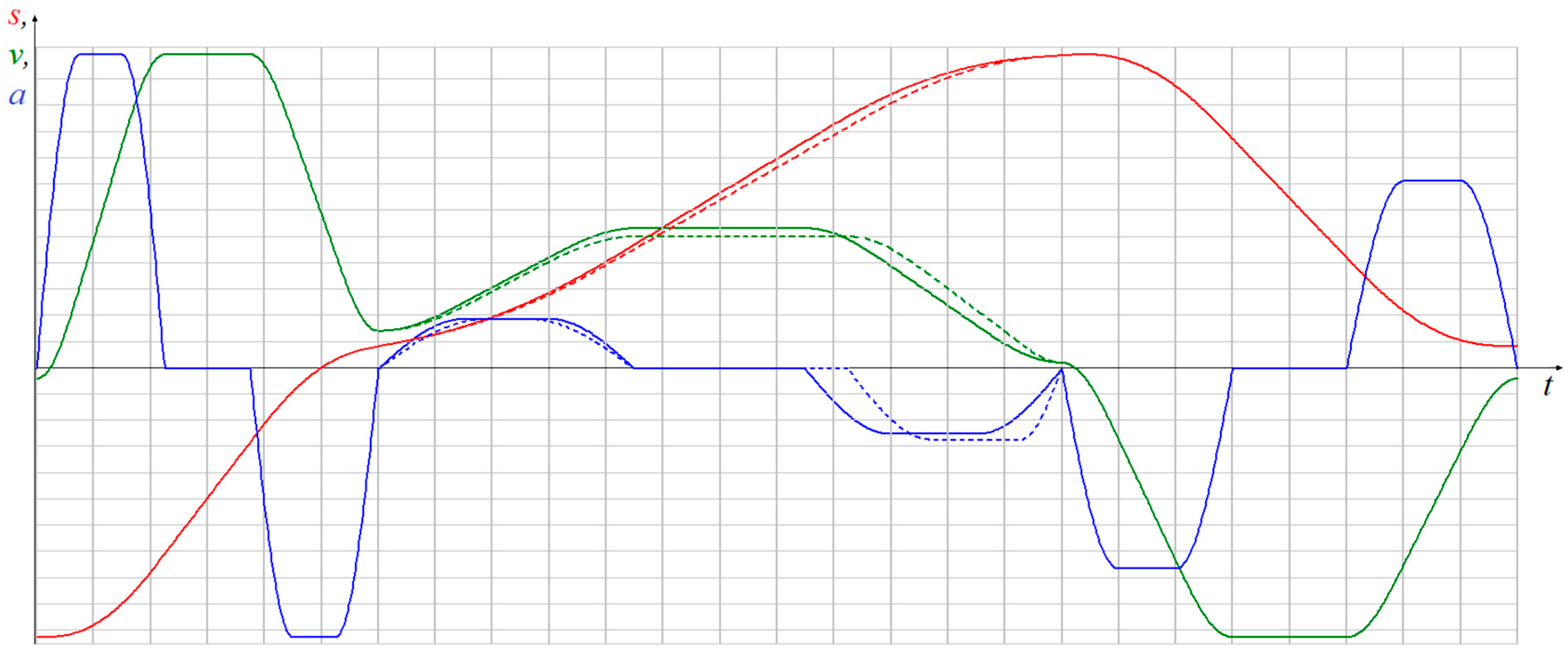
2.1. Laws of Motion and Motion Planning
2.2. Problem Definition and Genetic Algorithm Implementation
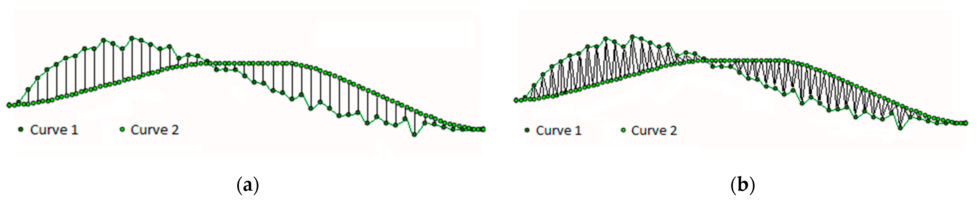
2.3. Objective Function
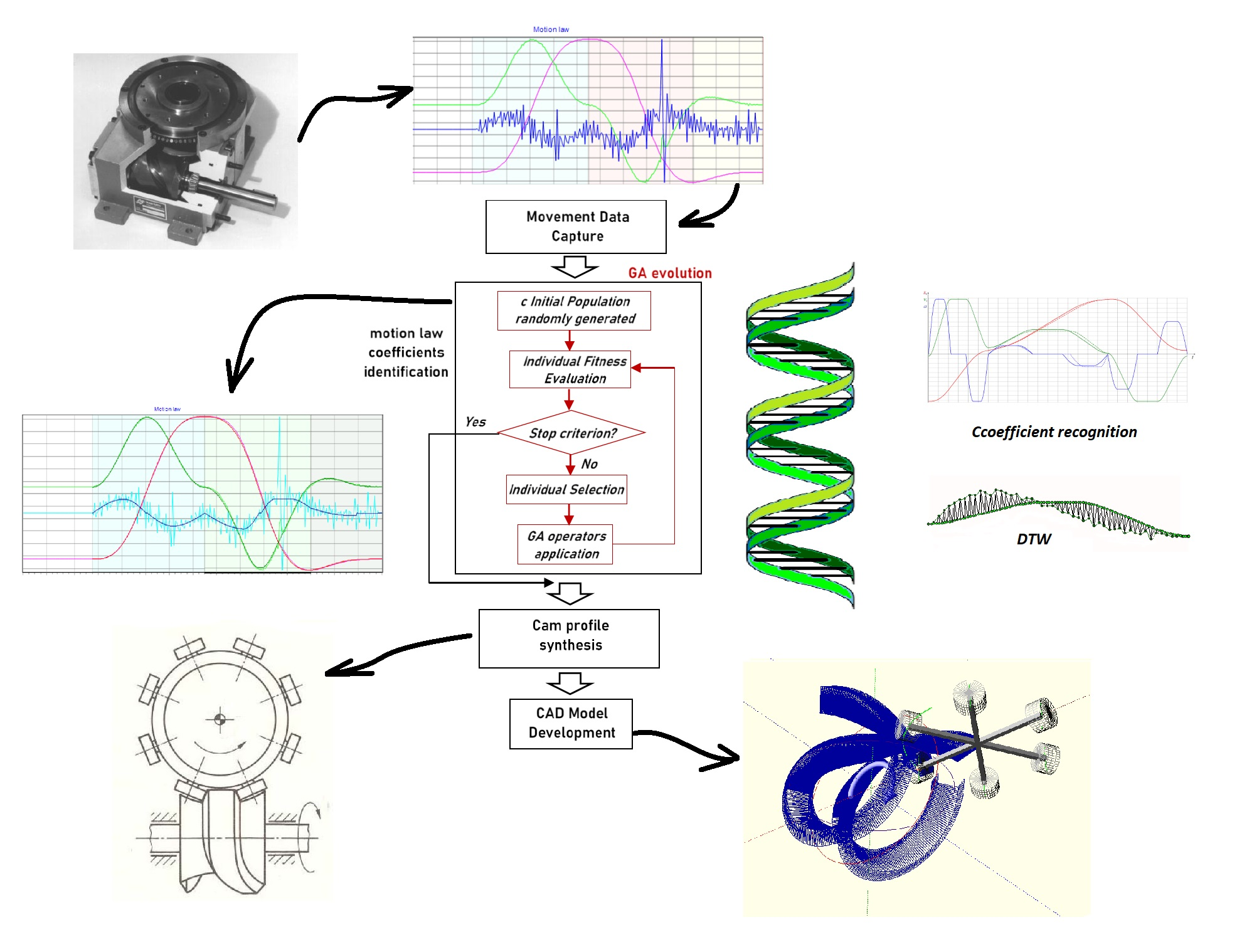
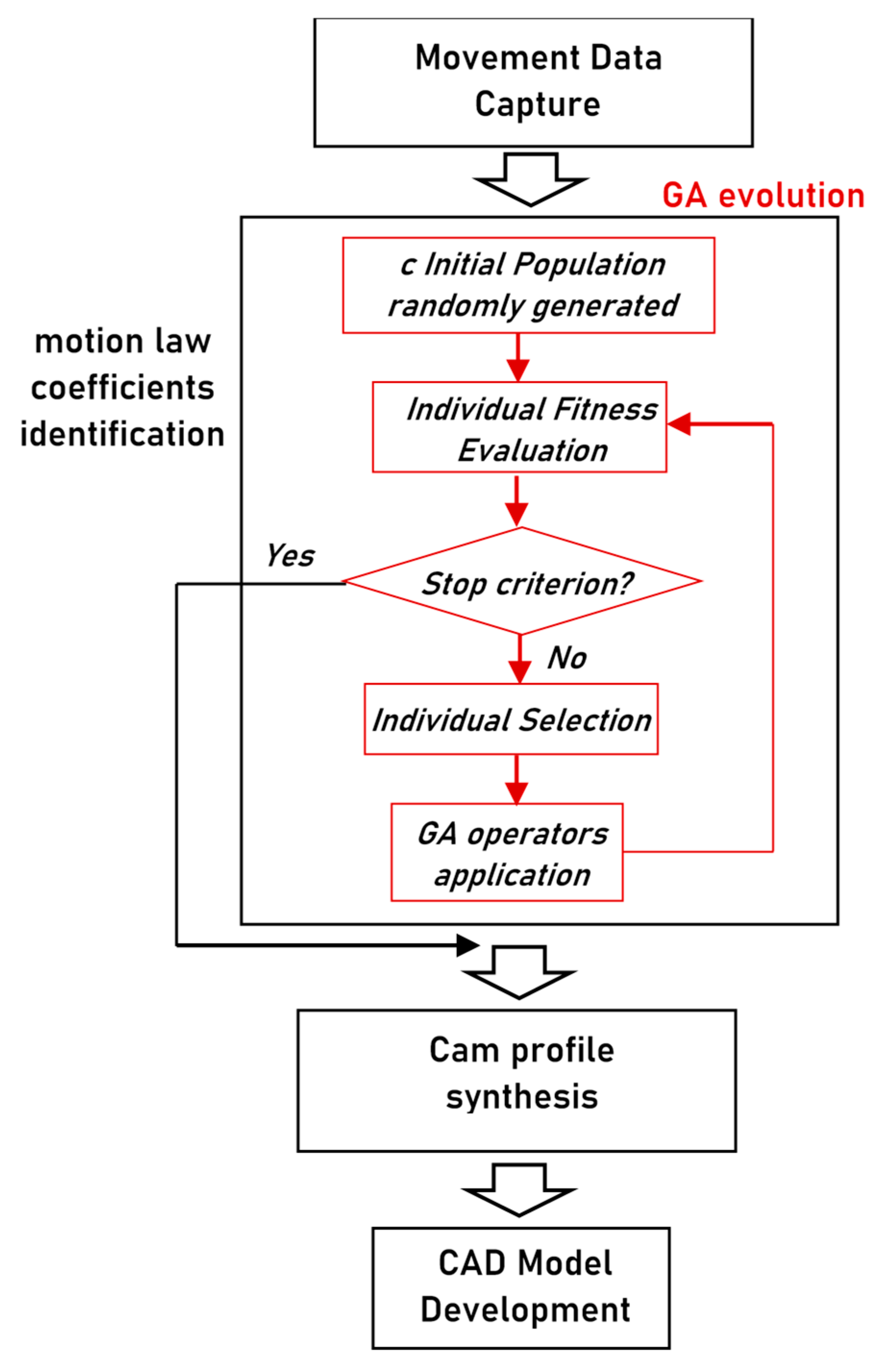
2.4. Developed Cam Mechanisms RE Framework
3. Results
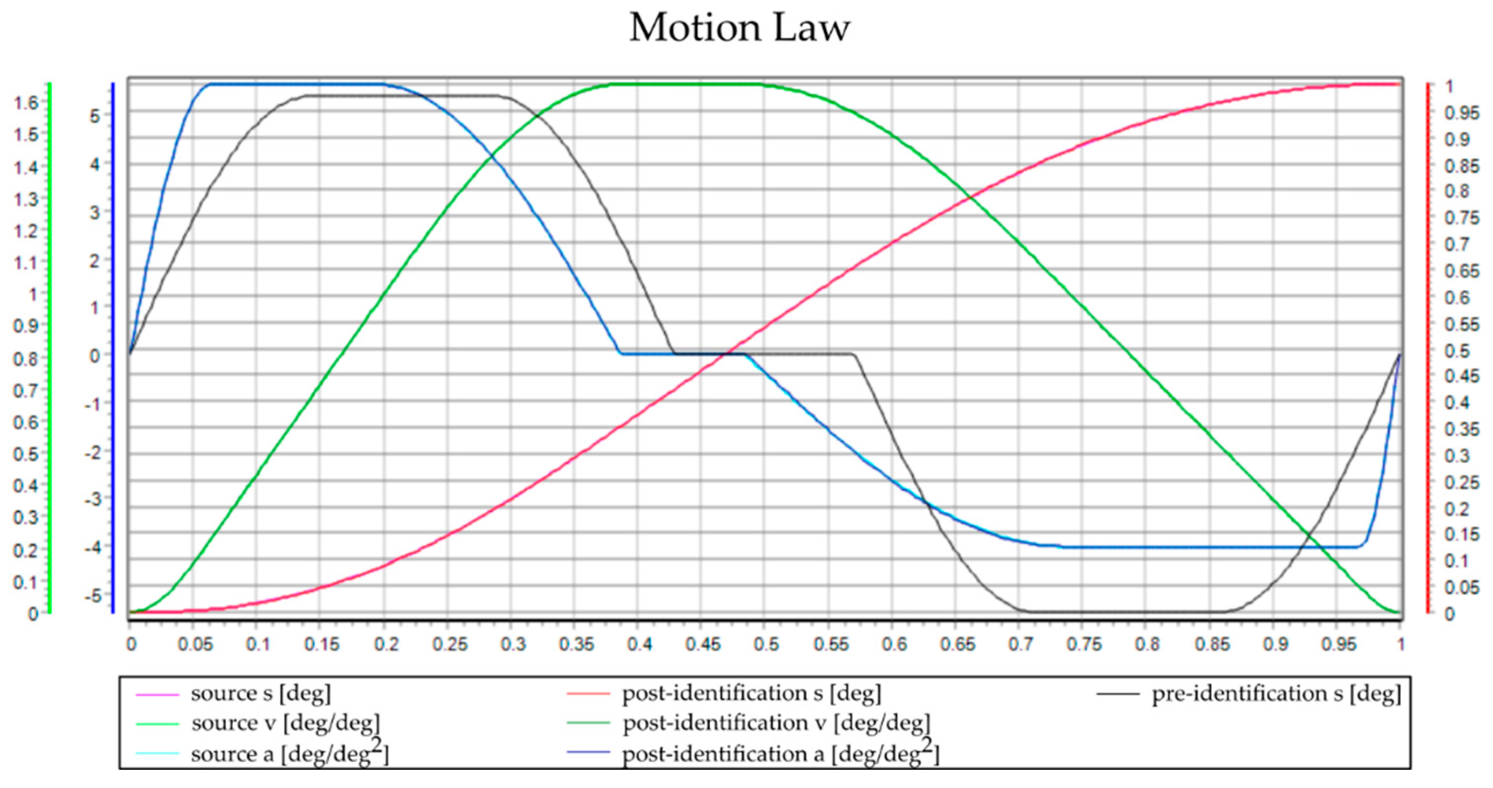
3.1. Simulations
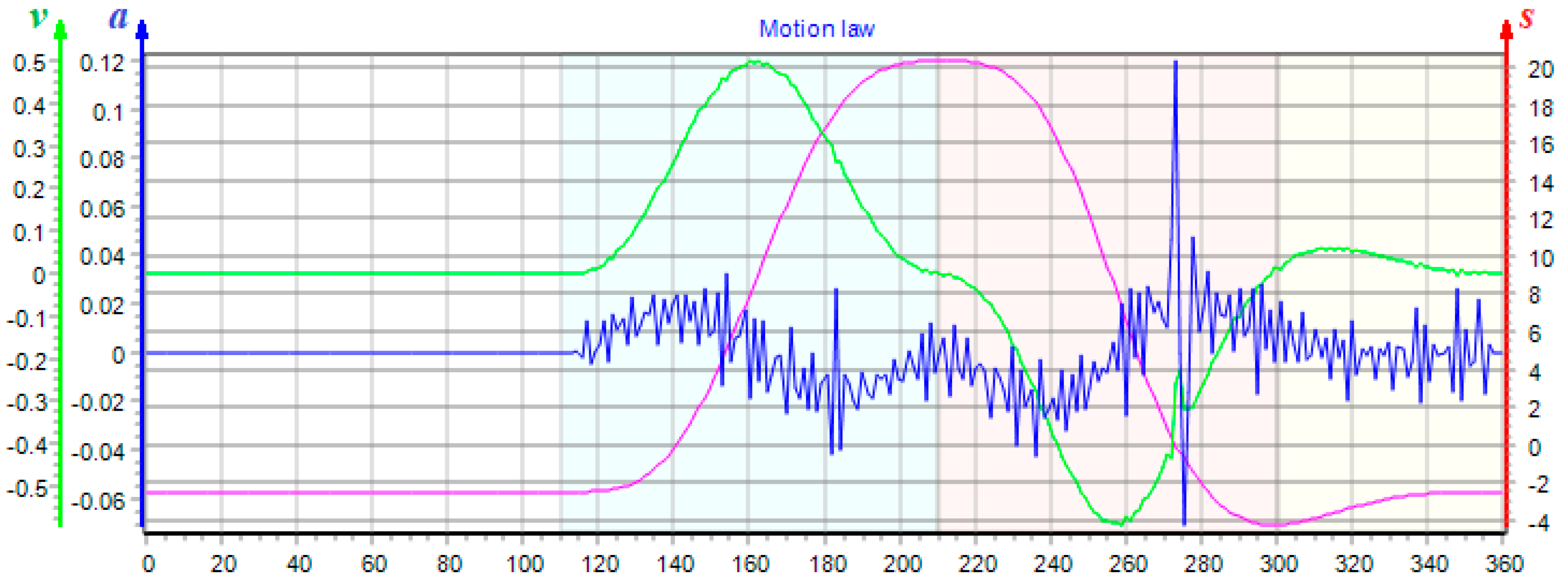
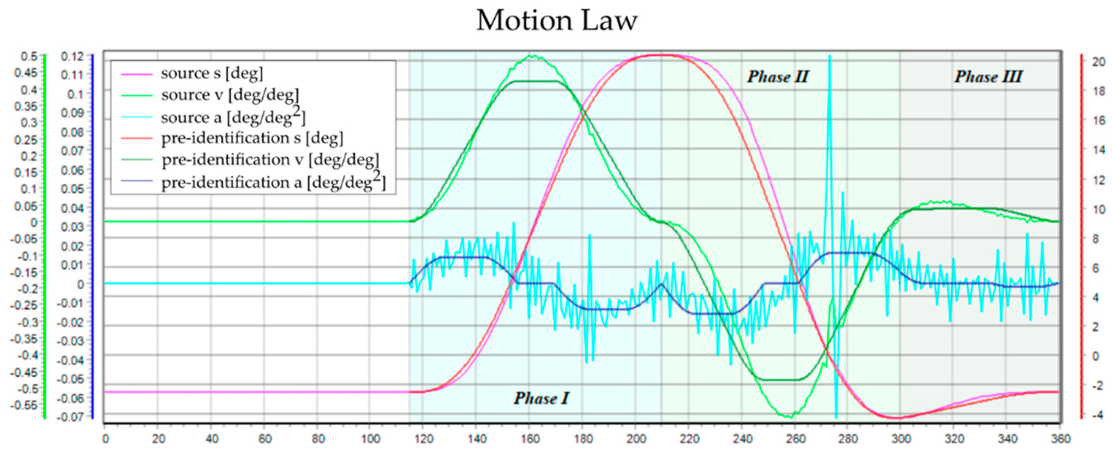
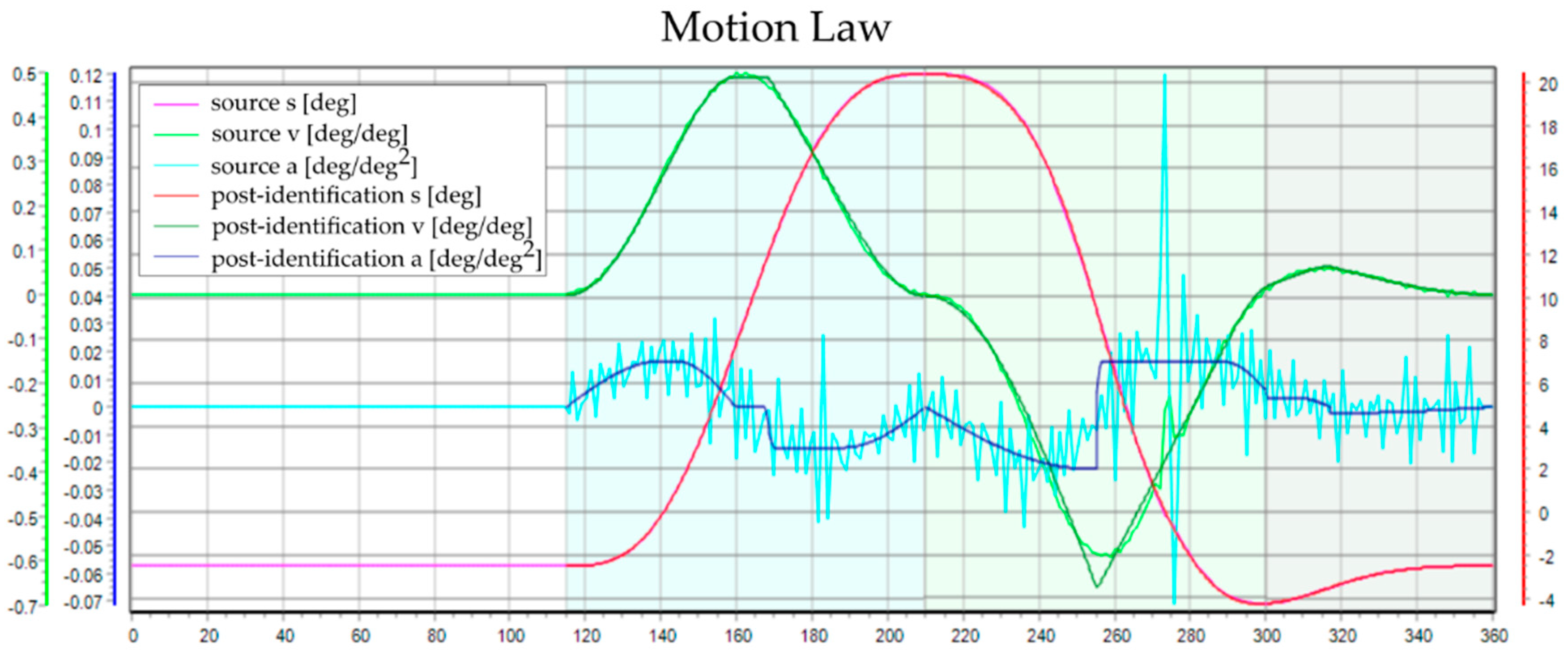
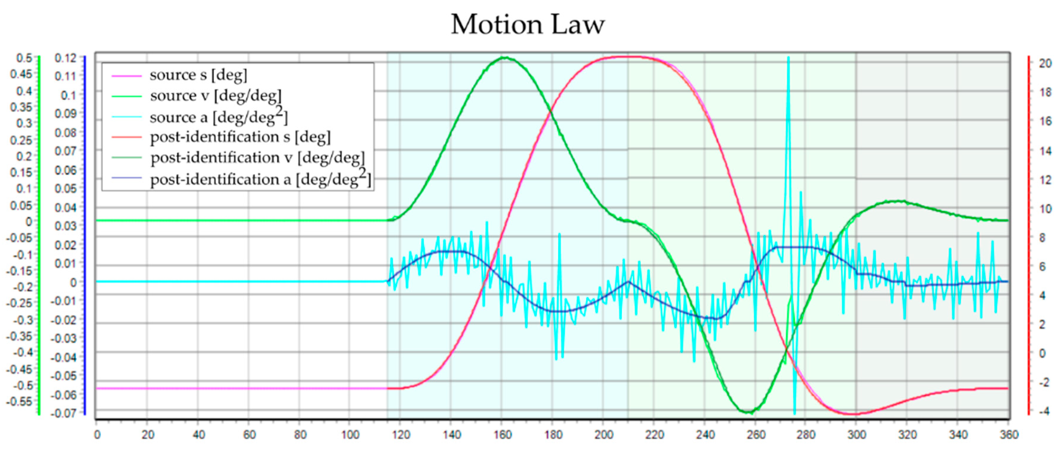
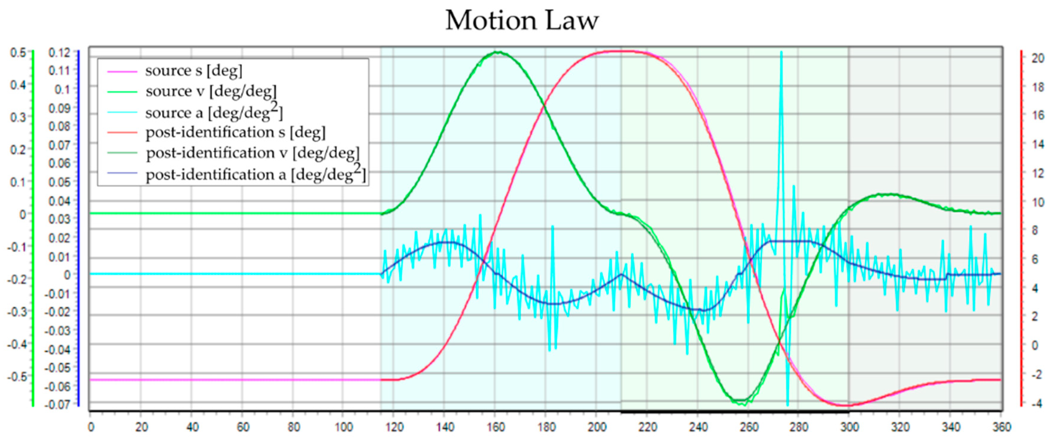
3.2. Tests on Experimental Data
4. Discussion
5. Conclusions
Author Contributions
Funding
Conflicts of Interest
Appendix A. Trapezoidal Modified Law of Motion

| Title 1 | Title 2 |
|---|---|
| Kinematic Quantity | Interval | Expression |
|---|---|---|
References
- Chen, F.Y. Mechanics and Design of Cam Mechanisms; Pergamon Press: Oxford, UK, 1982. [Google Scholar]
- Wilson, C.E.; Sadler, J.P.; Michels, W.J. Kinematics and Dynamics of Machinery; Pearson Edition: London, UK, 1983. [Google Scholar]
- Flores, P. A computational approach for cam size optimization of disc cam-follower mechanisms with translating roller followers. J. Mech. Robot. 2013, 5, 041010. [Google Scholar] [CrossRef] [Green Version]
- Abderazek, H.; Yildiz, A.R.; Mirjalili, S. Comparison of recent optimization algorithms for design optimization of a cam-follower mechanism. Knowl. Based Syst. 2020, 191, 105237. [Google Scholar] [CrossRef]
- Parouha, R.P.; Verma, P. Design and applications of an advanced hybrid meta-heuristic algorithm for optimization problems. Artif. Intell. Rev. 2021, 54, 5931–6010. [Google Scholar] [CrossRef]
- Lampinen, J. Cam shape optimisation by genetic algorithm. CAD Comput. Aided Des. 2003, 35, 727–737. [Google Scholar] [CrossRef]
- Tsiafis, I.; Mitsi, S.; Bouzakis, K.D.; Papadimitriou, A. Optimal design of a cam mechanism with translating flat-face follower using genetic algorithm. Tribol. Ind. 2013, 35, 255–260. [Google Scholar]
- Bhattacharjee, P.; Jana, R.K. A multi-objective genetic algorithm for design optimisation of simple and double harmonic motion cams. Int. J. Des. Eng. 2017, 7, 77–91. [Google Scholar] [CrossRef]
- Hamza, F.; Abderazek, H.; Lakhdar, S.; Ferhat, D.; Yıldız, A.R. Optimum design of cam-roller follower mechanism using a new evolutionary algorithm. Int. J. Adv. Manuf. Technol. 2018, 99, 1267–1282. [Google Scholar] [CrossRef]
- Yu, J.; Huang, K.; Luo, H.; Wu, Y.; Long, X. Manipulate optimal high-order motion parameters to construct high-speed cam curve with optimized dynamic performance. Appl. Math. Comput. 2020, 371, 124953. [Google Scholar] [CrossRef]
- Ouyang, T.; Wang, P.; Huang, H.; Zhang, N.; Chen, N. Mathematical modeling and optimization of cam mechanism in delivery system of an offset press. Mech. Mach. Theory 2017, 110, 100–114. [Google Scholar] [CrossRef]
- Gatti, G.; Mundo, D. On the direct control of follower vibrations in cam-follower mechanisms. Mech. Mach. Theory 2010, 45, 23–35. [Google Scholar] [CrossRef]
- Carbone, G.; Lanni, C.; Ceccarelli, M.; Incerti, G.; Tiboni, M. A characterization of cam transmissions through an identification of lumped parameters. Proc. ASME Des. Eng. Tech. Conf. 2006, 2006, 709–718. [Google Scholar] [CrossRef]
- Tiboni, M.; Bussola, R.; Aggogeri, F.; Amici, C. Experimental and model-based study of the vibrations in the load cell response of automatic weight fillers. Electronics 2020, 9, 995. [Google Scholar] [CrossRef]
- Tiboni, M.; Roberto, B.; Carlo, R.; Faglia, R.; Adamini, R.; Amici, C. Study of the Vibrations in a Rotary Weight Filling Machine. In Proceedings of the 2019 23rd International Conference on Mechatronics Technology, ICMT 2019, Salerno, Italy, 23–26 October 2019; pp. 1–6. [Google Scholar] [CrossRef]
- Dalpiaz, G.; Rivola, A. Condition monitoring and diagnostics in automatic machines: Comparison of vibration analysis techniques. Mech. Syst. Signal Process. 1997, 11, 53–73. [Google Scholar] [CrossRef] [Green Version]
- Tiboni, M.; Remino, C. Condition monitoring of a mechanical indexing system with artificial neural networks. In Proceedings of the WCCM 2017—1st World Congress on Condition Monitoring 2017, London, UK, 13–16 June 2017; Springer International Publishing: Berlin, Germany, 2017. [Google Scholar]
- Tiboni, M.; Incerti, G.; Remino, C.; Lancini, M. Comparison of signal processing techniques for condition monitoring based on artificial neural networks. Appl. Cond. Monit. 2019, 15, 179–188. [Google Scholar] [CrossRef]
- Buonamici, F.; Carfagni, M.; Furferi, R.; Governi, L.; Lapini, A.; Volpe, Y. Reverse engineering modeling methods and tools: A survey. Comput. Aided. Des. Appl. 2018, 15, 443–464. [Google Scholar] [CrossRef] [Green Version]
- Fu, P. Reverse Engineering in the Medical Device Industry; Springer International Publishing: Berlin, Germany, 2008; pp. 177–194. ISBN 978-1-84628-855-5. [Google Scholar]
- Balamurugan, P.; Selvakumar, N. Development of patient specific dental implant using 3D printing. J. Ambient Intell. Humaniz. Comput. 2021, 12, 3549–3558. [Google Scholar] [CrossRef]
- Chaudhary, K.; Govil, A. Application of 3D Scanning for Reverse Manufacturing and Inspection of Mechanical Components BT—Proceedings of the International Conference on Industrial and Manufacturing Systems (CIMS-2020); Pratap Singh, R., Tyagi, D.M., Panchal, D., Davim, J.P., Eds.; Springer International Publishing: Cham, Switzerland, 2020; pp. 61–76. [Google Scholar]
- Li, D. Application of Coordinate Measuring Machine in Reverse Engineering. Adv. Mater. Res. 2011, 301–303, 269–274. [Google Scholar] [CrossRef]
- Zhenghao, G.; Kaikai, Z.; Meng, J.; Fulian, Y. An Exact Reverse Design Approach for Disk Cam Mechanisms. Adv. Syst. Sci. Appl. 2011, 11, 301–308. [Google Scholar]
- Alsoufi, M.S.; Alhazmi, M.W.; Azam, S.; Modeling, C.A.D. Mechanical reverse engineering approach for precise measurements of reproducing disc CAM. Int. J. Eng. Technol. 2018, 7, 5741–5757. [Google Scholar] [CrossRef]
- Samsonenko, D.M.; Khudoyarov, V.A.; Barbashov, N.N.; Abdullina, L.R.; Potapov, D.M. Research of influence of errors of cam manufacturing on the law of motion of output element. IOP Conf. Ser. Mater. Sci. Eng. 2020, 862, 032053. [Google Scholar] [CrossRef]
- Goldberg, D.E. Genetic Algorithms in Search, Optimization and Machine Learning, 1st ed.; Addison-Wesley Longman Publishing Co., Inc.: Boston, MA, USA, 1989; ISBN 0201157675. [Google Scholar]
- Ratanamahatana, C.A.; Keogh, E. Making time-series classification more accurate using learned constraints. In Proceedings of the 2004 SIAM International Conference on Data Mining, Lake Buena Vista, FL, USA, 22–24 April 2004; Society for Industrial and Applied Mathematics: Philadelphia, PA, USA; pp. 11–22. [Google Scholar] [CrossRef] [Green Version]
- Yadav, M.; Alam, M.A. Dynamic Time Warping (DTW) Algorithm In Speech: A Review. Int. J. Res. Electron. Comput. Eng. 2018, 6, 524–528. [Google Scholar]
- Senin, P. Dynamic Time Warping Algorithm Review. Science 2008, 2007, 1–23. [Google Scholar]
- Gameros, A.; De Chiffre, L.; Siller, H.R.; Hiller, J.; Genta, G. A reverse engineering methodology for nickel alloy turbine blades with internal features. CIRP J. Manuf. Sci. Technol. 2015, 9, 116–124. [Google Scholar] [CrossRef]
- Wang, J.; Gu, D.; Yu, Z.; Tan, C.; Zhou, L. A framework for 3D model reconstruction in reverse engineering. Comput. Ind. Eng. 2012, 63, 1189–1200. [Google Scholar] [CrossRef]
- Wang, J.; Gu, D.; Gao, Z.; Yu, Z.; Tan, C.; Zhou, L. Feature-based solid model reconstruction. J. Comput. Inf. Sci. Eng. 2013, 13, 1–13. [Google Scholar] [CrossRef]
- Tsay, D.-M.; Huang, M.-H.; Ho, H.-C. Producing Follower Motions Through Their Digitized Cam Contours. J. Comput. Inf. Sci. Eng. 2002, 2, 98–105. [Google Scholar] [CrossRef]
- Ge, Z.; Su, P.; Yang, F.; Jiang, M. The Reverse Design Method for Cam Contours and Motion Specification. In Proceedings of the International Technology and Innovation Conference 2009 (ITIC 2009), Xi’an, China, 12–14 October 2009; pp. 1–4. [Google Scholar] [CrossRef]


| Parameter | Value |
|---|---|
| Constraints | |
| Normalized coefficients | |
| Number of sampled points | 300 |
| Parameter | Chosen Value |
|---|---|
| Number of genes for each individual | 7 |
| Number of individuals per generation | 100 |
| Probability of cross-over application | 0.85 |
| Inversion application probability | 0.1 |
| Probability of application of mutation around the range | 0.1 |
| Percentage of initial range mutation | 10% |
| Mutation range reduction | 75% each 50 generations |
| ID | Original Law of Motion | |||||||
|---|---|---|---|---|---|---|---|---|
| L1 | Modified Sinusoidal | 0.125 | 0 | 0.3750 | 0 | 0.3750 | 0 | 0.1250 |
| L2 | Constant Acceleration | 0 | 0.5000 | 0 | 0 | 0 | 0.5000 | 0 |
| L3 | Trimmed Constant Acceleration | 0 | 0.2500 | 0 | 0.5000 | 0 | 0.2500 | 0 |
| L4 | Cubic | 0 | 0 | 0.500 | 0 | 0.500 | 0 | 0 |
| L5 | Trapezoidal | 0.1250 | 0.2500 | 0.1250 | 0 | 0.1250 | 0.2500 | 0.1250 |
| L6 | Modified Trapezoidal | 0.1250 | 0.1250 | 0.1250 | 0.1250 | 0.1250 | 0.1250 | 0.1250 |
| L7 | Trimmed Trapezoidal | 0.0625 | 0.1250 | 0.0625 | 0.5000 | 0.0625 | 0.1250 | 0.0625 |
| L8 | Cycloidal | 0.2500 | 0 | 0.2500 | 0 | 0.250 | 0 | 0.2500 |
| L9 | Asymmetric Trapezoidal | 0.0500 | 0.2000 | 0.0500 | 0 | 0.050 | 0.6000 | 0.0500 |
| ID | Kinematic Quantity | Method | Max. Error | |||||||
|---|---|---|---|---|---|---|---|---|---|---|
| L1 | Acceleration | EN | 0.1218 | 0.0159 | 0.3598 | 0.0030 | 0.3598 | 0.0169 | 0.1226 | 0.0169 |
| DTW | 0.1240 | 0.0101 | 0.3617 | 0.0073 | 0.3683 | 0.0033 | 0.1250 | 0.0133 | ||
| Velocity | EN | 0.1246 | 0.0212 | 0.3513 | 0.0091 | 0.3521 | 0.0079 | 0.1335 | 0.0236 | |
| DTW | 0.0992 | 0.1131 | 0.2646 | 0.0464 | 0.2646 | 0.1118 | 0.1001 | 0.1131 | ||
| L2 | Acceleration | EN | 2.0 × 10⁻⁸ | 0.5000 | 0 | 0 | 0 | 0.5000 | 6.7 × 10⁻⁸ | 6.7 × 10⁻⁸ |
| DTW | 0 | 0.5000 | 1.3 × 10⁻⁹ | 1.5 × 10⁻⁹ | 1.3 × 10⁻¹ | 0.5000 | 0 | 1.5 × 10⁻⁹ | ||
| Velocity | EN | 0.0007 | 0.4922 | 0.0063 | 5.5 × 10⁻⁹ | 0.0100 | 0.4907 | 0 | 0.01000 | |
| DTW | 0.0113 | 0.4302 | 0.0536 | 0 | 0.0629 | 0.4302 | 0.0116 | 0.0697 | ||
| L3 | Acceleration | EN | 2.5 × 10⁻⁵ | 0.2499 | 0 | 0.5000 | 0.0030 | 0.2430 | 0.0039 | 0.0065 |
| DTW | 7.3 × 10⁻⁵ | 0.2506 | 5.8 × 10⁻⁵ | 0.4666 | 0.0889 | 0.1899 | 0.0038 | 0.0889 | ||
| Velocity | EN | 0.0020 | 0.2032 | 0.0682 | 0.4679 | 0.02410 | 0.2345 | 0.0001 | 0.0682 | |
| DTW | 0.0191 | 0.1000 | 0.1842 | 0.4020 | 0.1440 | 0.1480 | 0.0026 | 0.1841 | ||
| L4 | Acceleration | EN | 0 | 0.0003 | 0.4997 | 0.0002 | 0.4978 | 0.0018 | 1.4 × 10⁻⁸ | 0.0021 |
| DTW | 2.3 × 10⁻¹⁰ | 2.9 × 10⁻⁹ | 0.5 | 1.1 × 10¹⁰ | 0.5 | 0 | 1.8 × 10⁻⁹ | 2.9 × 10⁻⁹ | ||
| Velocity | EN | 6.8 × 10⁻⁸ | 0 | 0.5002 | 0.0018 | 0.4836 | 0.0139 | 0.0003 | 0.0163 | |
| DTW | 0.0019 | 0.0852 | 0.3910 | 0.0471 | 0.3922 | 0.0825 | 1.2 × 10⁵ | 0.1090 | ||
| L5 | Acceleration | EN | 0.1253 | 0.2494 | 0.1254 | 0 | 0.1246 | 0.2505 | 0.1248 | 0.0006 |
| DTW | 0.1250 | 0.2438 | 0.1348 | 0 | 0.1148 | 0.2565 | 0.12 | 0.0101 | ||
| Velocity | EN | 0.1244 | 0.2528 | 0.1218 | 8.6 × 10⁻⁵ | 0.1290 | 0.2465 | 0.1256 | 0.0039 | |
| DTW | 0.1414 | 0.2159 | 0.1432 | 0.0026 | 0.1303 | 0.2264 | 0.1402 | 0.0341 | ||
| L6 | Acceleration | EN | 0.1254 | 0.1240 | 0.1258 | 0.2498 | 0.1251 | 0.1248 | 0.1251 | 0.0010 |
| DTW | 0.1250 | 0.1251 | 0.1249 | 0.2451 | 0.138 | 0.1169 | 0.125 | 0.0130 | ||
| Velocity | EN | 0.1237 | 0.1297 | 0.1205 | 0.2474 | 0.1392 | 0.1113 | 0.1283 | 0.0141 | |
| DTW | 0.1460 | 0.0709 | 0.1636 | 0.2511 | 0.0871 | 0.1747 | 0.1065 | 0.0540 | ||
| L7 | Acceleration | EN | 0.0628 | 0.1240 | 0.0633 | 0.4998 | 0.0625 | 0.1246 | 0.0628 | 0.0009 |
| DTW | 0.0625 | 0.1249 | 0.0625 | 0.4952 | 0.0753 | 0.1169 | 0.0625 | 0.0128 | ||
| Velocity | EN | 0.0669 | 0.1008 | 0.0904 | 0.4870 | 0.0783 | 0.1115 | 0.0648 | 0.0278 | |
| DTW | 0.0619 | 0.1305 | 0.0556 | 0.5127 | 0.0176 | 0.1743 | 0.0478 | 0.0493 | ||
| L8 | Acceleration | EN | 0.2496 | 0.0010 | 0.2492 | 0.0005 | 0.2479 | 0.0029 | 0.2488 | 0.0029 |
| DTW | 0.2486 | 0.0102 | 0.2364 | 0.0093 | 0.2387 | 0.0076 | 0.2492 | 0.0136 | ||
| Velocity | EN | 0.2409 | 0.0335 | 0.2157 | 0.0194 | 0.2165 | 0.0335 | 0.2404 | 0.0342 | |
| DTW | 0.2169 | 0.0684 | 0.2125 | 0.0139 | 0.1829 | 0.0893 | 0.2159 | 0.0893 | ||
| L9 | Acceleration | EN | 0.0497 | 0.2008 | 0.0493 | 0 | 0.0508 | 0.5987 | 0.0505 | 0.0012 |
| DTW | 0.0500 | 0.2136 | 0.0246 | 0 | 0.1099 | 0.5460 | 0.0559 | 0.0598 | ||
| Velocity | EN | 0.0495 | 0.2322 | 0.0002 | 1.8 × 10⁻⁸ | 0.1075 | 0.5570 | 0.0534 | 0.0575 | |
| DTW | 0.0498 | 0.2273 | 0.0001 | 8.8 × 10⁻⁸ | 0.1666 | 0.4930 | 0.0630 | 0.1166 |
| Quantity | Method | Error | Noise | Err_s [Rad] | Err_v [Rad/s] | Err_a [Rad/s2] |
|---|---|---|---|---|---|---|
| Displacement | EN | EN | No | 0.0139 | 0.2542 | 7.5341 |
| DTW | No | 0.1036 | 1.2663 | 63.030 | ||
| DTW | EN | No | 0.0258 | 0.4078 | 12.022 | |
| DTW | No | 0.0726 | 2.4829 | 106.91 | ||
| Displacement | EN | EN | Yes | 0.0065 | 0.1816 | 21.771 |
| DTW | Yes | 0.0710 | 1.1354 | 294.62 | ||
| DTW | EN | Yes | 0.0291 | 0.4264 | 23.191 | |
| DTW | Yes | 0.0777 | 2.6604 | 330.20 | ||
| Velocity | EN | EN | No | 0.0025 | 0.0054 | 2.8170 |
| DTW | No | 0.0349 | 0.0562 | 16.730 | ||
| DTW | EN | No | 0.0073 | 0.1282 | 5.5620 | |
| DTW | No | 0.0548 | 0.3884 | 31.030 | ||
| Velocity | EN | EN | Yes | 0.0045 | 0.0666 | 20.530 |
| DTW | Yes | 0.0668 | 0.6859 | 284.00 | ||
| DTW | EN | Yes | 0.0119 | 0.1505 | 22.270 | |
| DTW | Yes | 0.1272 | 0.7712 | 292.20 | ||
| Acceleration | EN | EN | No | 0.0004 | 0.0036 | 0.1068 |
| DTW | No | 0.0060 | 0.0477 | 1.0890 | ||
| DTW | EN | No | 0.0026 | 0.0254 | 1.2838 | |
| DTW | No | 0.0320 | 0.1572 | 2.2197 | ||
| Acceleration | EN | EN | Yes | 0.0163 | 0.0853 | 21.103 |
| DTW | Yes | 0.2278 | 1.0417 | 291.66 | ||
| DTW | EN | Yes | 0.0400 | 0.2240 | 20.877 | |
| DTW | Yes | 0.2184 | 2.1890 | 283.13 |
| Error | Polynomial 3-3 | Polynomial 4-4 | Polynomial 5-5 | ||||||
|---|---|---|---|---|---|---|---|---|---|
| Err_s [Rad] | Err_v [Rad/s] | Err_a [Rad/s2] | Err_s [Rad] | Err_v [Rad/s] | Err_a [Rad/s2] | Err_s [Rad] | Err_v [Rad/s] | Err_a [Rad/s2] | |
| EN | 0.0828 | 0.7645 | 11.91 | 0.4886 | 3.646 | 35.32 | 0.784 | 6.011 | 58.23 |
| DTW | 0.346 | 6.609 | 125.7 | 6.098 | 48.69 | 533.026 | 10.19 | 82.64 | 875.06 |
| Kinematic Quantity | Method | Error | Polynomial 3-3 | Polynomial 4-4 | Polynomial 5-5 | ||||||
|---|---|---|---|---|---|---|---|---|---|---|---|
| Err_s [Rad] | Err_v [Rad/s] | Err_a [Rad/s2] | Err_s [Rad] | Err_v [Rad/s] | Err_a [Rad/s2] | Err_s [Rad] | Err_v [Rad/s] | Err_a [Rad/s2] | |||
| Disp. | EN | EN | 0.010 | 0.273 | 7.619 | 0.0567 | 0.815 | 22.040 | 0.191 | 2.060 | 45.940 |
| DTW | 0.142 | 2.288 | 84.20 | 0.522 | 8.242 | 269.5 | 2.020 | 25.800 | 560.300 | ||
| DTW | EN | 0.062 | 0.632 | 10.71 | 0.075 | 1.015 | 19.250 | 0.194 | 2.077 | 46.230 | |
| DTW | 0.116 | 5.188 | 107.9 | 0.498 | 12.24 | 236.600 | 2.020 | 25.90 | 563.900 | ||
| Velocity | EN | EN | 0.004 | 0.086 | 2.642 | 0.747 | 0.682 | 13.220 | 0.225 | 1.817 | 29.700 |
| DTW | 0.059 | 1.057 | 25.90 | 0.680 | 6.645 | 171.800 | 2.438 | 22.590 | 412.500 | ||
| DTW | EN | 0.013 | 0.191 | 4.020 | 0.075 | 0.699 | 11.330 | 0.216 | 1.844 | 30.520 | |
| DTW | 0.132 | 0.787 | 45.42 | 0.649 | 6.422 | 149.300 | 2.290 | 22.200 | 329.900 | ||
| Accel. | EN | EN | 0.007 | 0.064 | 1.388 | 0.112 | 0.808 | 9.423 | 0.288 | 2.137 | 22.680 |
| DTW | 0.109 | 0.650 | 11.81 | 1.026 | 8.956 | 112.900 | 3.250 | 28.810 | 302.500 | ||
| DTW | EN | 0.015 | 0.104 | 1.540 | 0.114 | 0.822 | 9.217 | 0.295 | 2.187 | 29.410 | |
| DTW | 0.195 | 0.770 | 8.780 | 1.051 | 9.217 | 111.300 | 3.330 | 22.750 | 298.600 | ||
| Phase Name | Constraint Vector | [Deg] | [Deg] | [Deg] | [Deg] | [Deg/Deg] | [Deg/Deg] | [Deg/Deg2] | [Deg/Deg2] |
|---|---|---|---|---|---|---|---|---|---|
| Phase I | 115.0 | 210.0 | −2.5000 | 20.3800 | 0.0 | 0.0 | 0.0 | 0.0 | |
| Phase II | 210.0 | 300.0 | 20.3800 | −4.2700 | −0.0028 | 0.0183 | 0.0 | 0.0060 | |
| Phase III | 300.0 | 360.0 | −4.2700 | −2.500 | 0.0 | 0.0 | 0.0060 | 0.0 |
| Quantity | Method | Error | Phase I | Phase II | Phase III | ||||||
|---|---|---|---|---|---|---|---|---|---|---|---|
| Err_s [Deg] | Err_v [Deg/ Deg] | Err_a [Deg/ Deg2] | Err_s [Deg] | Err_v [Deg/ Deg] | Err_a [Deg/ Deg2] | Err_s [Deg] | Err_v [Deg/ Deg] | Err_a [Deg/ Deg2] | |||
| None | EN | 7.083 | 0.590 | 0.187 | 17.600 | 1.090 | 1.370 | 2.868 | 0.221 | 0.169 | |
| DTW | 77.500 | 7.393 | 2.551 | 193.300 | 14.020 | 7.310 | 36.060 | 3.186 | 2.080 | ||
| EN | EN | 0.364 | 0.130 | 0.178 | 1.977 | 0.545 | 1.390 | 0.104 | 0.057 | 0.167 | |
| Displacement | DTW | 4.662 | 1.181 | 2.446 | 18.270 | 3.962 | 7.076 | 0.764 | 0.683 | 2.007 | |
| DTW | EN | 0.490 | 0.127 | 0.178 | 1.811 | 0.599 | 1.392 | 0.120 | 0.062 | 0.172 | |
| DTW | 3.250 | 1.111 | 2.450 | 11.060 | 5.137 | 7.171 | 0.760 | 0.757 | 2.148 | ||
| EN | EN | 1.587 | 0.080 | 0.176 | 4.220 | 0.512 | 1.389 | 0.219 | 0.052 | 0.167 | |
| Velocity | DTW | 3.601 | 0.734 | 2.420 | 40.020 | 3.399 | 7.017 | 1.404 | 0.626 | 2.085 | |
| DTW | EN | 2.132 | 0.070 | 0.176 | 2.870 | 0.520 | 1.389 | 0.210 | 0.052 | 0.167 | |
| DTW | 7.835 | 0.592 | 2.42 | 24.840 | 3.130 | 6.980 | 1.276 | 0.621 | 2.000 | ||
| Accel. | EN | EN | 1.165 | 0.076 | 0.176 | 4.059 | 0.520 | 1.389 | 1.068 | 0.077 | 0.166 |
| DTW | 8.189 | 0.672 | 2.414 | 38.030 | 3.458 | 6.984 | 13.410 | 0.959 | 2.077 | ||
| DTW | EN | 2.404 | 0.122 | 0.177 | 2.779 | 0.592 | 1.389 | 1.657 | 0.147 | 0.167 | |
| DTW | 13.093 | 1.084 | 2.406 | 21.195 | 4.458 | 6.950 | 20.380 | 2.009 | 2.039 | ||
| Phase Name | Coefficient Vector | |||||||
|---|---|---|---|---|---|---|---|---|
| Phase I | 0.2386 | 0.0566 | 0.1867 | 0.0126 | 0.2121 | 0.0 | 0.2933 | |
| Phase II | 0.3917 | 0.0500 | 0.1195 | 0.0235 | 0.1199 | 0.1389 | 0.2065 | |
| Phase III | 0.0027 | 0.0620 | 0.1691 | 0.0890 | 0.0028 | 0.0002 | 0.6740 |
Publisher’s Note: MDPI stays neutral with regard to jurisdictional claims in published maps and institutional affiliations. |
© 2021 by the authors. Licensee MDPI, Basel, Switzerland. This article is an open access article distributed under the terms and conditions of the Creative Commons Attribution (CC BY) license (https://creativecommons.org/licenses/by/4.0/).
Share and Cite
Tiboni, M.; Amici, C.; Bussola, R. Cam Mechanisms Reverse Engineering Based on Evolutionary Algorithms. Electronics 2021, 10, 3073. https://doi.org/10.3390/electronics10243073
Tiboni M, Amici C, Bussola R. Cam Mechanisms Reverse Engineering Based on Evolutionary Algorithms. Electronics. 2021; 10(24):3073. https://doi.org/10.3390/electronics10243073
Chicago/Turabian StyleTiboni, Monica, Cinzia Amici, and Roberto Bussola. 2021. "Cam Mechanisms Reverse Engineering Based on Evolutionary Algorithms" Electronics 10, no. 24: 3073. https://doi.org/10.3390/electronics10243073