Mapping Chlorophyll-a Concentrations in the Kaštela Bay and Brač Channel Using Ridge Regression and Sentinel-2 Satellite Images

Abstract

In this paper, we describe a method for the prediction of concentration of chlorophyll-a (Chl-a) from satellite data in the coastal waters of Kaštela Bay and the Brač Channel (our case study areas) in the Republic of Croatia. Chl-a is one of the parameters that indicates water quality and that can be measured by in situ measurements or approximated as an optical parameter with remote sensing. Remote sensing products for monitoring Chl-a are mostly based on the ocean and open sea monitoring and are not accurate for coastal waters. In this paper, we propose a method for remote sensing monitoring that is locally tailored to suit the focused area. This method is based on a data set constructed by merging Sentinel 2 Level-2A satellite data with in situ Chl-a measurements. We augmented the data set horizontally by transforming the original feature set, and vertically by adding synthesized zero measurements for locations without Chl-a. By transforming features, we were able to achieve a sophisticated model that predicts Chl-a from combinations of features representing transformed bands. Multiple Linear Regression equation was derived to calculate Chl-a concentration and evaluated quantitatively and qualitatively. Quantitative evaluation resulted in $R^2$ scores 0.685 and 0.659 for train and test part of data set, respectively. A map of Chl-a of the case study area was generated with our model for the dates of the known incidents of algae blooms. The results that we obtained are discussed in this paper.

1. Introduction

Coastal water quality monitoring is an important activity for retrieving information about the state of a marine ecosystem. In the Republic of Croatia, the degree of sea bathing water quality is regulated by the Regulation on Sea bathing water quality (OG 73/08) and the EU Directive on management of bathing water quality No 2006/7/EC. Consequently, it is necessary to constantly monitor the quality of the sea and the cleanliness of the coast, primarily because of human and animal health, fishing, and also because of tourism as one of the main economic incomes and activities of people on the Adriatic coast, especially in the summer season [1]. This is why responsible authorities schedule in situ measurements of various water quality indicators for continuous, albeit sparse, monitoring.

One of the indicators that depicts the quality of marine and freshwater is the concentration of Chlorophyll-a (Chl-a). Besides merely showing the quality of the water, Chl-a can also be used as a proxy for phytoplankton biomass and that is why it is an indicator of water quality and trophic status [2]. This is why it is important to continuously monitor Chl-a in a body of water.

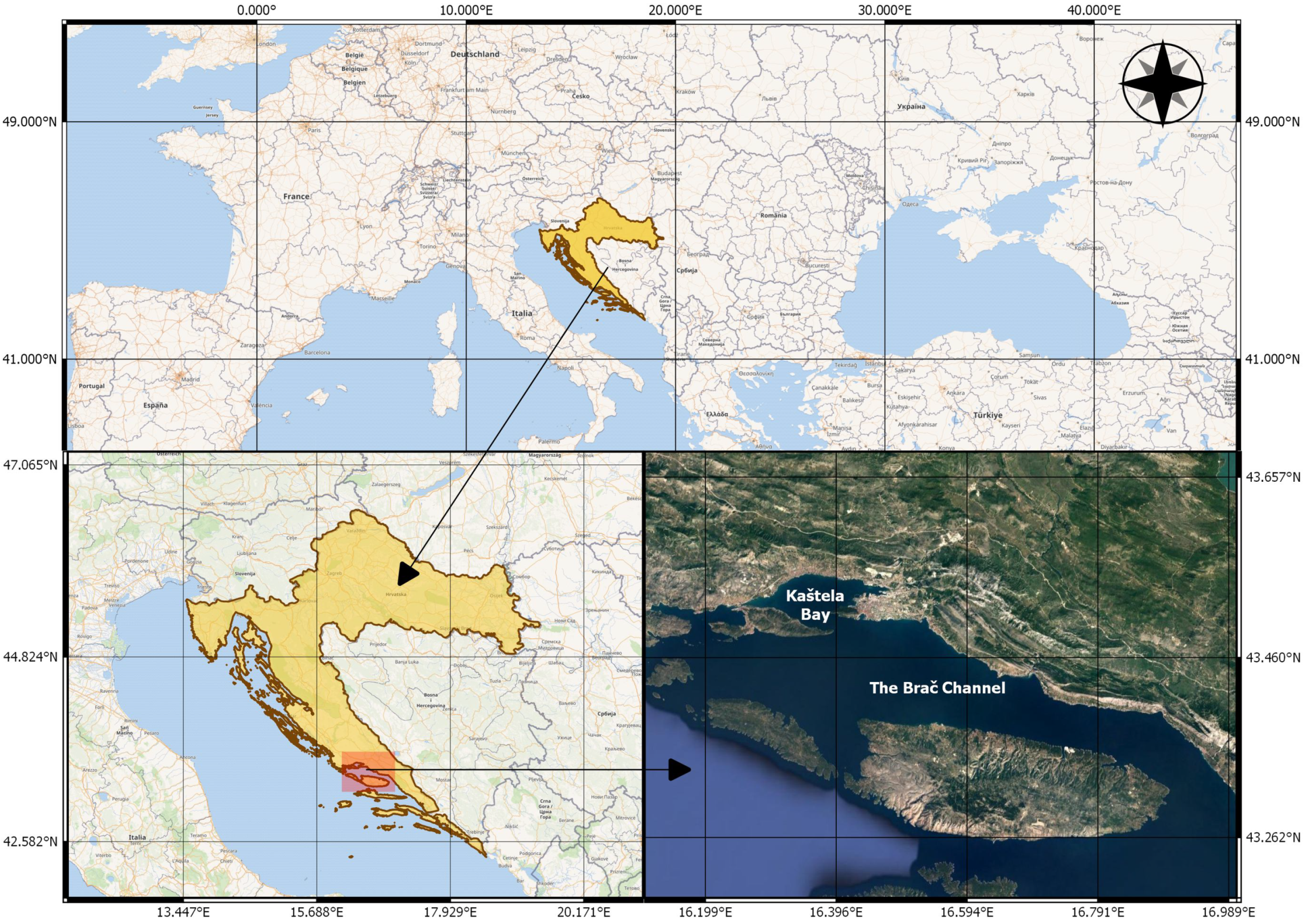
In this study, we analyzed the possibility of estimating Chl-a in coastal environments, specifically in the Kaštela Bay and the Brač Channel in Croatia, by using satellite remote sensing to complement the existing in situ monitoring with continuous and more frequent assessment.

Characteristics of the coastal environment result in the complexity of the marine ecosystem and pose challenges to the monitoring of water quality indices. Increases in natural or anthropogenic nutrients result in higher concentrations of phytoplankton and marine organisms, which we measure as a concentration of Chl-a [3]. The concentration of Chl-a is usually measured by taking samples of water and making laboratory analysis of collected samples. This way, we can establish the concentration level for only a limited number of points of the research area, which makes this approach not only expensive and weather-dependent but also does not provide a broader picture of the distribution of Chl-a concentration [4].

Thus, in this paper, we offer an approach to calculate Chl-a concentration using the images obtained by Sentinel-2 satellite instruments. With this approach, we can obtain a broader picture of Chl-a distribution and concentrations because Chl-a is an optically active component that has a characteristic spectral signature allowing its detection with optical sensors onboard satellites. Moreover, Chl-a is connected with important processes in the sea (e.g., eutrophication and algae blooms); so, with remote sensing, continuous monitoring of changes in the sea becomes possible.

1.1. Related Work

Water quality monitoring using multispectral or hyperspectral remote sensing represents a great challenge in order to find the relationship between in situ data and reflectances obtained by various sensors. There are many optical and nonoptical parameters that affect water quality and can be estimated using satellite data [5,6]. The main research focus is on the optical properties of water such as chlorophyll [7], turbidity [8], total suspended matters [9], and colored dissolved organic matters [10], which affect the reflected radiation of the sea and, thus, can be measured remotely.

Many studies show a different usage of observations and methods for retrieving the concentration of Chl-a for different types of monitored waters. The widely used Ocean color (OC3) algorithm for the calculation of Chl-a concentration based on three bands (B01, B02, and B03), representing blue to green ratios, was proposed in [11]. This algorithm is an empirical, with parameters trained on data originating from ocean and coastal waters. Fitted parameters are published for various satellites. Sentinel-2 parameters are published in [12]. Case-2 Regional/Coast Colour (C2RCC) [13] is a physics-based processor for the calculation of various water parameters (such as Chl-a, total suspended matter (TSM), and colored dissolved organic matter (CDOM)). This algorithm utilizes a neural network trained on a large amount of data for inverting top-of-atmosphere (TOA) radiance to water-leaving reflectance. Implementation for various satellites is available as a part of ESA’s Sentinel Toolbox SNAP [14]. Types of water studied by various researches are lakes, rivers, oceans, estuaries, and coastal waters. Studies focus on certain study areas and use only certain satellite data. Methods for estimating parameters vary from fitting a formula parameter to machine learning algorithms. In [15], authors compared Sentinel-2A and Earth Observing-1 (EO1) for estimation of Chl-a and turbidity, where Sentinel-2A showed better results in retrieving concentration for both parameters (Chl $R^2$: 0.72 vs. 0.57 and TU $R^2$: 0.7 vs. 0.63). Further, the authors used reflectance ratio for mapping Chl-a, which can be seen in several other studies using different reflectance values for developing algorithms [2,16,17]. Sentinel-2 and Landsat-8 have good spatial resolution, which makes them suitable for monitoring the water quality along the coast [12,18,19,20,21], as opposed to Sentinel-3, SeaWiFS (Sea-Viewing Wide Field-of-View Sensor), and MODIS (Moderate Resolution Imaging Spectroradiometer), which have large spatial resolutions better for monitoring the open sea [22,23,24].

Several studies show that using regression models can have a big potential for retrieving the concentration of Chl-a in coastal environments and lakes [15,25,26,27,28]. For example, the authors in [3] compared predictive performance on three different regression models (Simple Linear Regression—SLR, Multiple Linear Regression—MLR, and Generalized Additive Models—GAMs) and Landsat-8 imagery. The results showed that GAM outperformed SLR and MLR, while the MLR performed better in predicting log-transformed Chl-a values. Furthermore, in [29], the authors compared Ordinary Least Square (OLS) with Ridge Regression (OPT) to estimate Chl-a, turbidity, and suspended sediment based on relationship with Landsat reflectance. Ridge Regression estimation showed better results compared with Ordinary Least Square analysis.

1.2. Proposed Method

The aim of this paper is to reveal the correlation between in situ Chl-a data and Sentinel-2 satellite band reflectance data using Ridge Regression for estimating the coefficients of Multiple Linear Regression to retrieve Chl-a concentration. The aforementioned studies used only predefined formulas and bands to develop a predictive model, while we present a regression model that takes all of the Sentinel-2 band reflectance data into account. Our modeling approach is purely data-oriented and aimed towards discovering the formula from the available data. The implemented regression model provided coefficients to create a formula used to estimate Chl-a concentration, which will be presented as a map of Chl-a distribution in the area of the Kaštela Bay and the Brač Channel revealing the spatial distribution of the Chl-a parameter and overall state of the aquatorium.

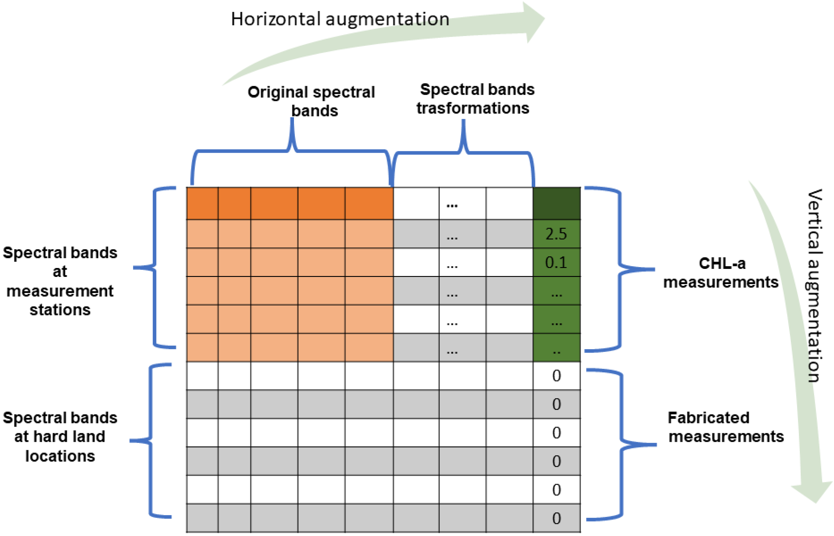
The main contribution of this paper is a novel method for developing a sophisticated and reliable model for predicting Chl-a from Sentinel-2. The developed model is tailored specifically for the study area. This is achieved by augmenting the original data set in two dimensions—horizontally (by performing feature augmentation by transforming the feature values) and vertically (by adding value 0 to the Chl-a measurements for the locations on land without Chl-a). The horizontal augmentation improved the correlation of predicted and measured Chl-a concentrations by providing a more sophisticated model with nonlinear dependencies on the spectral reflectances. The vertical augmentation enriched the data set with new data items. In this way, the regression algorithm receives not only the features of locations with Chl-a concentration but the locations without the Chl-a as well, making the data set more balanced. This method enabled creation of a model that is sophisticated and fitted to the features of the study area. Although the model is precisely fitted for the case study area and past measurements, the evaluation of the model shows that our model does not overfit. The reliability of the model is qualitatively validated on the algae bloom incident. Finally, the two novel contributions of the paper can be summed up as follows:

• A method for developing a sophisticated formula for estimation of Chl-a values in coastal waters where we have a limited number of measurements.
• A new regression formula for estimating Chl-a concentrations in coastal waters of study area.

2. Materials and Methods

2.1. Study Area

Figure 1 shows the study area, which is located in the Kaštela Bay and the Brač Channel, near Split—the second largest city in the Republic of Croatia. Both locations are coastal water bodies. Kaštela Bay is the largest bay in central Dalmatia and it is about 14.8 km-long, 6.6 km-wide and up to 60 m-deep [30]. The river Jadro (near the city of Solin) and the stream Pantana (near the city of Trogir) flow into the bay. The Brač Channel is a sea passage between the mainland of Dalmatia and the island of Brač, and is about 50 km-long, 5 to 13 km-wide and up to 78 m-deep. The river Cetina in the city of Omiš flows into the Brač Channel, which deposits sand and creates a shoal that stretches up to 800 m from the shore [31]. The study area location is depicted in Figure 1. Water body of this area is a swimming area for many tourists and local citizens during warm summer periods, and also an area of rich biodiversity for fishery [32]. Due to the high number of people living on the shore of this area, this is also one of the most vulnerable areas when analyzing the risk of pollution. Two rivers in the study area (Jadro and Cetina) bring pollution and nutrients that feed the sea microorganisms responsible for sea blooms. Another cause of higher Chl-a is sewage discharged into the sea, so feces cause contaminants such as the presence of coliform bacteria, e.g., Escherichia Coli and Enterococci. All of these various types of pollution affect animal and human health, and cause economical problems related to tourism and fishing. It is, therefore, necessary to monitor and react timely to these problems, especially in the summertime when it is a swimming season.

2.2. In Situ Data Set

The in situ measurements were performed by Hrvatske Vode, a legal entity for water management in the Republic of Croatia. The samples were collected over the study area on thirteen different stations (Figure 2) and at different depths (0 m, 5 m, 10 m, 20 m, 30 m, and 50 m) during the years 2017, 2018, and 2019. The sea sampling frequency was once a month and performed in the middle of each month on dates depending on weather conditions. Not all thirteen stations were included in each measurement. For 2017 and 2019, each measurement in one month was performed for seven different stations, and for 2018, measurements were performed for six different stations. Besides Chl-a, other water quality parameters were measured from the samples, but in the scope of this paper we will focus only on Chl-a.

Table 1. Summary statistic of in situ Chlorophyll-a values.

Station	N	Latitude	Longitude	Minimum	Maximum	Mean	Standard Deviations
S01	25	43.503411	16.208292	0.11	0.97	0.41	0.21
S02	20	43.541706	16.401844	0.07	1.36	0.62	0.36
S03	42	43.53	16.453333	0.19	2.28	0.81	0.40
S04	6	43.5359	16.46885	0.19	1.79	0.75	0.49
S05	7	43.53409722	16.47113056	0.24	1.5	0.61	0.38
S06	6	43.53319444	16.48310556	0.26	4.35	1.27	1.33
S07	55	43.518333	16.381667	0.07	1.56	0.58	0.37
S08	16	43.503183	16.433797	0.26	1.13	0.55	0.19
S09	15	43.488367	16.436667	0.09	1.54	0.39	0.32
S10	34	43.426719	16.393519	0.07	1.63	0.38	0.28
S11	10	43.42385	16.673533	0.10	0.59	0.31	0.16
S12	11	43.432356	16.682061	0.09	0.56	0.31	0.16
S13	7	43.444792	16.690806	0.21	3.13	1.14	0.95

shows the Chl-a concentration statistics for all thirteen measurement stations.

The Chl-a concentration was measured by the fluorimetric method, where the samples were filtered under vacuum up to 65 KPa through Whatman GF/C glass filters, with a pore diameter of about 1 µm. The devices used to determine the concentration of Chl-a were a centrifuge, a TD-700 fluorimeter, and a homogenizer. The sample volume ranges from 200 to 500 mL, depending on the area and sampling season. The total number of samples for all years of measurements, stations, and depths is 480.

It is important to stress that the in situ Chl-a measurement was performed by a team from the national authority for water management, and followed the official standard procedure as prescribed in [33]. The data set consisting of in situ measurements was obtained via official channels and delivered to us via e-mail from a representative of the legal entity that owns the data. In the scope of this paper, we consider the values provided by the in situ Chl-a measurement as ground truth values and have no reason to doubt the validity of measurement. All presented results are based on the assumption that the in situ measurements are accurate and precise.

Since Chl-a is a pigment that is optically active and produces a characteristic spectral signature, we are interested in the concentration of Chl-a that can be detected using optical sensors onboard satellites. We did not only use the value of Chl-a concentration measured on the sea surface, but we also took into account the values measured at different depths. Remotely sensed values depend on the concentration of Chl-a in the water column that is visible to the sensor. Thus, we used in situ Chl-a measurements on depths lower than measured Secchi depth. The values of the Secchi depth were also measured in situ on the same dates and locations as the Chl-a measurements. After we calculated the mean Chl-a value for each station based on the Chl-a concentration data for different depths that are lower than the measured Secchi depth value, the final set of in situ data was constructed and contained 121 measurement values.

2.3. Satellite Data

The Sentinel-2 is an Earth observation mission comprised of a constellation of two identical satellites (Sentinel-2A and Sentinel-2B). It has a revisit time of 5 days of the same area using both satellites. Further, both of these satellites contain a MultiSpectral Instrument (MSI) that can sample 13 spectral bands. The spatial resolutions and central wavelengths [34] of the 13 spectral bands of Sentinel-2 are shown in

Table 2. Spatial resolution and central wavelength of each band of Sentinel-2 images.

Band	Spatial Resolution (m)	Central Wavelength (nm)
B01	60	443
B02	10	490
B03	10	560
B04	10	665
B05	20	705
B06	20	740
B07	20	783
B08	10	842
B8A	20	865
B09	60	945
B10	60	1375
B11	20	1610
B12	20	2190

.

In this study, we used Sentinel Level-2A atmospherically corrected data products. The Level-2A product provides Bottom of Atmosphere (BOA) reflectance images that are processed from associated Level-1C images with Sen2Cor processor [35]. We did not consider different atmospheric correction procedures nor any other available satellite products indicating the data quality, besides filtering outliers indicating clouds. In the scope of this paper, we only focused on finding the correlations between band values and measured Chl-a values regardless of other parameters. Final images are available from Sentinel Hub API [36].

We obtained a high-quality image where the influence of the atmosphere on the light that reaches the sensor reflects from the Earth’s surface. We collected 3024 TIFF (32-bit float) images of all bands except band B10, which was not available through Sentinel Hub at the time of writing of this paper. A total of 252 different scenes covering the study area for 2017, 2018, and 2019 were taken for processing. The cloud coverage of each scene is less than 20%. Images were downloaded from the Sentinel Hub EO Browser [36] page by implementing a script in the Python programming language that uses the API requests (credit: Modified Copernicus Sentinel data 2017/Sentinel Hub). Due to the higher time resolution of the Sentinel-2 satellite, we could not retrieve the satellite image for the exact day of each sampling, so we retrieved the images of the nearest day the image was available, either before or after the sampling date.

2.4. Methodology

The methodology includes several stages required to obtain results. Based on the described and collected in situ and satellite data, we created a data set on which data transformations were applied. After building the data set, we applied Ridge Regression on the data set and constructed a Multiple Linear Regression (MLR) formula to estimate Chl-a concentrations in our study area.

2.4.1. Data Set Construction

Figure 3 shows the initial procedure for collecting in situ and satellite data for constructing a data set, as described in the previous sections. Data set of in situ Chl-a values has been constructed by aggregating the mean value of the measured Chl-a for different depths that are less than the measured Secchi depth. In this way, we calculate the mean Chl-a concentration of each measurement at thirteen individual stations. The range of the measured Chl-a value is between 0.1475 μg/L and 2.435 μg/L (average value of 0.596281 μg/L) for all three years of measurement (2017, 2018, and 2019).

To retrieve satellite data, we downloaded 32-bit float .tiff Sentinel Level-2A satellite images of each band georeferenced in the WGS 84 coordinate system (EPSG: 4326).

For all in situ measurement stations, we read a value of each Sentinel Level-2A band from the image. Since the image contains 16-bit numbers ranging up to 65,535, we applied a factor of 1/10,000 similar to [37] on pixel values in order to obtain a value capable of storing and manipulation.

In situ and satellite data were merged based on the measurement station and the date of the sampling and observation.

For the dates when in situ measurement missions were carried out, we selected Sentinel Level-2A images for each available band and extracted band values at the pixels associated with the location of the measurement station. In this way, we associated 12 band reflectance values with one Chl-a measurement value. Since the Sentinel-2 revisit period for the study area is 5 days, we wanted to check the time difference between the sampling and observation. In our final data set, 82% of images were obtained on the same day as thein situ measurement, 12% with one day difference, and for the rest of the data we allowed up to 10 days difference. We tested the performance by allowing only the smaller difference but no significant improvement of the algorithm was noticed; so, we decided to keep the data of up to 10 day difference in order to feed the machine learning algorithm with more data. The distribution of time differences of the used data set is shown in Figure 4. For comparison, Sentinel 3 revisit time is one day, so we would be able to obtain an image on each day of the measurement but with the cost of lower spatial resolution of the images.

This resulted in a data set of a total of 118 records representing band values associated with in situ Chl-a samples.

Table 3. Summary statistics of Chlorophyll-a and band values.

N = 118	Minimum	Maximum	Mean	Standard Deviations
B01	0.0007	6.5535	0.6344	1.0987
B02	0.0380	6.3595	0.6079	1.0585
B03	0.0131	6.1288	0.5567	0.9901
B04	0.0039	6.2861	0.4706	0.9772
B05	0.0059	6.4309	0.5171	1.0122
B06	0.0013	6.2887	0.5437	1.019
B07	0.0059	6.2665	0.5608	1.0238
B08	0.0125	6.4277	0.5714	1.0905
B09	0.0020	6.5535	0.7290	1.4344
B11	0.0026	3.5835	0.4883	0.7806
B12	0.0013	3.1627	0.3980	0.6392
B8A	0.0026	6.2075	0.5770	1.0353
ChlA	0.0700	2.0500	0.5361	0.3730

contains descriptive statistics of associated in situ Chl-a and band values. The span of minimal and maximal values and standard deviation show that the dataset contains diverse values. This was expected since the measuring stations are located on 13 different geographical locations and the measurements are performed during three years.

2.4.2. Multiple Linear Regression Model

Multiple linear regression (MLR) is a statistical modeling technique that extends simple linear regression. This model was built in order to predict a response variable (y) from multiple explanatory variables ($x_1,x_2,\dots ,x_n$) [38]. The goal of this model is to represent a linear relationship between many independent predictor variables (bands) and a single dependent variable (Chl-a) as a single functional formula [39]. The equation [40] for the MLR model is as follows (1):

$$y={\beta }_0+{\beta }_1{x}_1+...+{\beta }_n{x}_n$$

(1)

where

• y is a dependent variable, which, in our case, is a concentration of Chlorophyll-a;
• β₀ is a constant, often referred to as bias or intercept;
• β_i is a regression coefficient for an independent variable $X_i$; and
• x_{i(i=1,2,…,n)} are independent variables that are, in our case, the values of Sentinel-2 reflectance bands.

Multiple linear regression modeling is a task of finding the optimal values of ${\beta }_0$ intercept and ${\beta }_i$ coefficients to make the prediction more accurate.

2.4.3. Ridge Regression

Multicollinearity is the existence of a nearly linear relationship between regression variables, predictor variables, or input/exogenous variables [41]. It may lead to inaccurate estimates of regression coefficients [42] when using traditional regression modeling methods. To avoid this problem, we used a statistical technique called Ridge Regression, which was first introduced by Hoerl and Kennard [43]. The concept of this method is based on the Least Squares Estimator (LSE), reducing the mean square error and retrieving a more stabilized regression coefficients [29]. Ridge Regression Estimator (RRE) of $\beta$ [41] is defined in (2) for the multiple linear model (1):

$${\widehat{\beta }}_n^{RR}\left(k\right)={(C+k{I}_p)}^{-1}{X}^{T}Y,C=X^{T}X$$

(2)

where

• ${\widehat{\beta }}_n^{RR}$ is a regression coefficient;
• X is an independent variable that presents a design matrix;
• Y is a response vector;
• k is a tuning parameter; k$\in [0,\infty \rangle$; and
• I_p is identity matrix.

The equation above shows that the ridge $\beta$s change with k-value and become the same as LSE $\beta$s if k is equal to zero.

2.4.4. Statistical Evaluation Indices

The evaluation of the predictive performance of Ridge Regression Estimator model was evaluated based on several criteria such as the coefficient of multiple determination ($R^2$) and Root Mean Square Error (RMSE).

The $R^2$ metric [44], also called Pearson squared correlation, is equal to the square of the correlation coefficient and represents a linear consistency. Thus, proportion of the variation and the in situ and Sentinel Level-2A observations as a linear consistency is explained by the linear regression. This metric can be calculated as follows (3):

$$R^2=\frac{{\sum }_{i=1}^n{(\widehat{y_i}-\overline{y})}^2}{{\sum }_{i=1}^n{(y_i-\overline{y})}^2}=1-\frac{{\sum }_{i=1}^n{(y_i-\widehat{y_i})}^2}{{\sum }_{i=1}^n{(y_i-\overline{y})}^2}$$

(3)

where $y_i$ is the value of the ith sample, $\overline{y}$ represents the mean of variable y, and $\widehat{y_i}$ is the estimated value of the ith sample [44].

RMSE is used to measure the difference between the estimated value of the estimator and the actual value. This is the perfect measure of accuracy for comparing the difference in prediction errors from different estimators on a given variable [45]. The equation [46] for this measure can be seen in (4):

$$RMSE=\sqrt{\frac{1}{N}\sum _{i=1}^N{(y_i-x_i)}^2}$$

(4)

In the shown equation, $x_i$ represents the ith in situ observation, $y_i$ represents the ith value predicted by the algorithm based on Sentinel Level-2A observation, and N is the number of match-ups.

2.4.5. Data Set Augmentation

Data set augmentation [47] is a process often used to increase the performance of machine learning algorithms. Performance of the algorithm depends on the data set provided. Feeding algorithms with a larger data set results in more accurate predictions. Since obtaining new data items is not always easy, authors synthetically expand a training set using augmentation techniques. Data set augmentation refers to simple and complex transformation of data items in a dataset in order to obtain a larger set of data and achieve better performance of a machine learning algorithm.

In our approach, we applied data set augmentation in two directions, which is illustrated in Figure 5. The original data set we collected consists of spectral values at the measuring stations measured by instrument on Sentinel-2 satellite (orange part) and Chl-a values measured at the same measuring stations (green part). The original data set is augmented among two axes—horizontal and vertical. With vertical augmentation, we increased the number of rows in the data set by adding fictional measurements on hard land where we are sure that the concentration of Chl-a is zero. With horizontal augmentation, we increased the number of columns in the data set by adding new features that are achieved by transforming the original features.

2.4.6. Vertical Augmentation

Vertical augmentation was performed by adding new fictional measurements to the data set of in situ Chl-a measurements. We fabricated in situ measuring stations for Chl-a on arbitrary locations where we were sure that the Chl-a concentration is always zero. We selected coordinates for these fabricated measuring stations to be located on landmarks such as airports, rooftops, and stone pits in the case study area. We selected a total of six such locations in order to make our data set more balanced.

In further processing, these fictional measurements were treated the same as real measurements with Chl-a concentration measured to be zero. Our intuition was that, besides enriching the data set with more data, these new data items will teach the algorithm the features of locations that do not have Chlorophyll. As we will show later, this resulted in the exclusion of objects on the sea (such as boats) and land from mapping Chl-a concentrations.

2.4.7. Horizontal Augmentation

Some variables do not conform to assumptions of linear relationship, normality, independence, and homoscedasticity of error terms, which may produce misleading results [48]. Since Ridge Regression is limited only on linear relationship of exploratory variables and result, we performed feature augmentation on bands to increase and change the data set. Each band is taken as a special feature in the data set. In this way, our data set is expanded horizontally by adding four different transformations on features values: logarithmic transformation, square transformation, square root transformation, and reciprocal transformation, as can be seen in (5), (6), (7) and (8), respectively:

$$valLog={log}_{10}\left(B_i\right)$$

(5)

$$valSquare=B_i^2$$

(6)

$$valRoot=\sqrt{B_i}$$

(7)

$$valRec=\frac{1}{B_i}$$

(8)

where B_i represents each band value (B01-B09, B11-B12, and B8A). Transformation is the application of a mathematical function to each value in a data set, where each set value is replaced by a transformed value, which can generally be written as in (9).

$$y=f\left(B_i\right)$$

(9)

Performed data transformations (vertical and horizontal) result in a data set with overall 60 features denoting bands reflectances and one feature related to Chl-a concentration. In this way, we have enriched the data set, so that the model has enough data to learn and can provide better accuracy by using a more complex prediction function.

3. Results

Ridge Regression model was developed on the constructed data set in a way of training the model on 80% of the data set, and testing and validating the model on the remaining 20% of the data set. Train set and Test set were constructed by randomly shuffling and splitting items into 80% and 20% of items, respectively. Further, we evaluated the constructed model and results using two approaches:

• Quantitative evaluation was performed on training and testing portions of the data set;
• Qualitative evaluation was performed by inspecting resulting images of Chl-a distribution for certain dates and discussing in the scope of the known events.

First, we wanted to make sure that the vertical augmentation we used on our data set is a valid approach and will yield better results. We developed a model on the original data set of 12 features and evaluated the model score. Then, we developed a model trained on the 80% of the vertically augmented data set including fabricated chlorophyll-free stations, and evaluated the model score. The results shown in

Table 4. Analysis of Ridge regression performance on original and vertically augmented data sets.

Number of Items	Data Set	${\mathit{R}}^2$	RMSE
118 (Original)	Train	0.0163	0.3290
	Test	0.0046	0.4672
328 (Vertically Augmented)	Train	0.4727	0.3031
	Test	0.4544	0.2190

indeed show better values of evaluation measures for both train and test portions of the data set for the model trained with vertically augmented data set. The percentage of data taken for training (80%) and testing (20%) is the same for each constructed data set.

Furthermore, in order to objectively verify that the horizontal augmentation is a valid approach to our problem, we trained the Ridge Regression model and observed the results for five different variations of features, from original bands to bands with all four data transformations applied.

This way, we ensured that the Ridge Regression model is not overfitted with additional features.

Table 5. Analysis of Ridge regression performance on different features, where $B_i$ represents a value of each Sentinel-2 band (B01-B09, B8A, and B11-12).

Features	Data Set	${\mathit{R}}^2$	RMSE
$B_i,i=\{1,\dots ,12\}$	Train	0.4727	0.3031
	Test	0.4544	0.2190
$B_i,{\left(B_i\right)}^{2}i=\{1,\dots ,12\}$	Train	0.6147	0.2202
	Test	0.6008	0.3257
$B_i,{\left(B_i\right)}^2,log\left(B_i\right)i=\{1,\dots ,12\}$	Train	0.6236	0.2689
	Test	0.6350	0.2512
$B_i,{\left(B_i\right)}^2,log\left(B_i\right),\sqrt{B_i}i=\{1,\dots ,12\}$	Train	0.6277	0.2271
	Test	0.6266	0.2836
$B_i,{\left(B_i\right)}^2,log\left(B_i\right),\sqrt{B_i},\frac{1}{B_i},i=\{1,\dots ,12\}$	Train	0.6850	0.2254
	Test	0.6599	0.2051

shows combinations of bands and transformations that we used for incremental Ridge Regression model testing. The model shows the most accurate results by taking into account all of the transformed features and original band values. The $R^2$ metric for train data is 0.685 and for test data is 0.6599, while RMSE metric is 0.2254 for train and 0.2051 for test data. This shows that Chl-a is quite correlated with transformed reflectance values of Sentinel-2 bands.

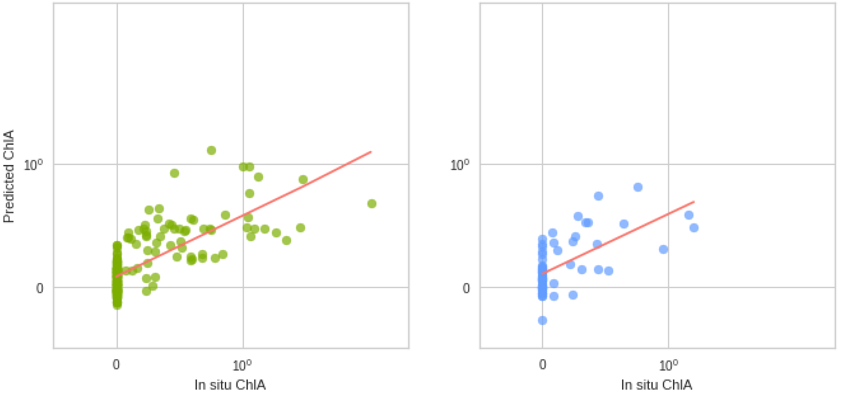
Figure 6 shows the relationship between values of in situ and predicted Chl-a values in the form of an error plot. From the error plot, we can notice that for both the test and the train data, the predicted values of Chl-a follow the same trend. Although the prediction is not perfectly accurate, for measurements with higher values of Chl-a, predicted values are higher, while for measurements with low Chl-a, predicted values are lower. For a certain number of measurements denoted as zero Chl-a, we have low predicted Chl-a but not exactly zero since for these points’ reflectances are measured on land, which has different behavior than the sea.

The predictions are made using a formula based on Equation (10).

$$\begin{array}{cc}\hfill ChlA(\mathsf{\mu }\mathrm{g}/\mathrm{L})& =b+{\displaystyle \sum _{i=1}^{12}}{\alpha }_i{\beta }_i+{\displaystyle \sum _{i=1}^{12}}{\gamma }_i{\beta }_i^2\hfill \\ \hfill & +{\displaystyle \sum _{i=1}^{12}}{\delta }_i\sqrt{{\beta }_i}+{\displaystyle \sum _{i=1}^{12}}{\theta }_i\frac{1}{{\beta }_i}+{\displaystyle \sum _{i=1}^{12}}{\varphi }_i\mathit{log}{\beta }_i\hfill \end{array}$$

(10)

where

• b represents intercept (bias), which is 0.2647;
• β₁, …, β₁₂ represents a reflectance value of each band (B01-B09, B11-B12, and B8A) divided by 10,000 and coefficients ${\alpha }_i$, ${\gamma }_i$, ${\delta }_i$, ${\theta }_i$, ${\varphi }_i$ are listed in

  Table 6. Estimated coefficients from Ridge Regression model.

  ${\mathit{\alpha }}_{\mathit{i}}$	${\mathit{\gamma }}_{\mathit{i}}$	${\mathit{\delta }}_{\mathit{i}}$	${\mathit{\theta }}_{\mathit{i}}$	${\mathit{\varphi }}_{\mathit{i}}$
  ${\alpha }_1$ = 0.2451	${\gamma }_1$ = −0.0686	${\delta }_1$ = 0.0382	${\theta }_1$ = 0.0001	${\varphi }_1$ = −0.0079
  ${\alpha }_2$ = 0.0747	${\gamma }_2$ = −0.0057	${\delta }_2$ = −0.0921	${\theta }_2$ = −0.1053	${\varphi }_2$ = −0.3762
  ${\alpha }_3$ = −0.0171	${\gamma }_3$ = −0.0553	${\delta }_3$ = −0.0442	${\theta }_3$ = 0.0013	${\varphi }_3$ = 0.1658
  ${\alpha }_4$ = −0.0516	${\gamma }_4$ = 0.1721	${\delta }_4$ = −0.1596	${\theta }_4$ = −0.0001	${\varphi }_4$ = −0.2753
  ${\alpha }_5$ = −0.0321	${\gamma }_5$ = 0.0774	${\delta }_5$ = −0.1365	${\theta }_5$ = −0.0032	${\varphi }_5$ = −0.1732
  ${\alpha }_6$ = −0.0517	${\gamma }_6$ = −0.2569	${\delta }_6$ = −0.1073	${\theta }_6$ = 0.0035	${\varphi }_6$ = −0.0486
  ${\alpha }_7$ = 0.0440	${\gamma }_7$ = −0.1091	${\delta }_7$ = −0.0820	${\theta }_7$ = −0.00003	${\varphi }_7$ = −0.0969
  ${\alpha }_8$ = −0.0128	${\gamma }_8$ = 0.0763	${\delta }_8$ = −0.0855	${\theta }_8$ = −0.0014	${\varphi }_8$ = 0.0106
  ${\alpha }_9$ = 0.0892	${\gamma }_9$ = 0.0204	${\delta }_9$ = −0.0072	${\theta }_9$ = 0.0003	${\varphi }_9$ = 0.2031
  ${\alpha }_{10}$ = 0.0496	${\gamma }_{10}$ = 0.0465	${\delta }_{10}$ = −0.2303	${\theta }_{10}$ = 0.0003	${\varphi }_{10}$ = 0.0025
  ${\alpha }_{11}$ = −0.1300	${\gamma }_{11}$ = −0.0366	${\delta }_{11}$ = −0.1964	${\theta }_{11}$ = −0.0006	${\varphi }_{11}$ = −0.1228
  ${\alpha }_{12}$ = 0.2741	${\gamma }_{12}$ = 0.1559	${\delta }_{12}$ = 0.0312	${\theta }_{12}$ = 0.0001	${\varphi }_{12}$ = 0.1713

  .

Equation (10) is constructed as a Multiple Linear Regression for estimating Chl-a concentration, where the coefficients are obtained by training the Ridge Regression model. Every feature represents either original or transformed band where every feature shows different correlation with in situ Chl-a. The coefficients can be considered as weights showing what influence the feature has on final output. For original band values (${\alpha }_i$), the most correlated bands are B01, B8A, and B12, while transformed features show the best correlation as follows:

• Squared features (${\gamma }_i$) for bands B04, B06, B07, and B8A;
• Squared root features (${\delta }_i$) for bands B04, B11, and B12;
• Reciprocal transformed features (${\theta }_i$) for band B02;
• Logarithmic transformed features (${\varphi }_i$) for bands B04, B05, and B8A.

Among selected features, we noticed that three of the transformed features of band B04 (${\left(B04\right)}^2$, $\sqrt{B04}$, and $log\left(B04\right)$) have higher coefficients. B04 is usually used in combination with vegetation red edge. Values of bands B05 or B8A are often proposed for retrieving Chl-a in coastal waters [21] or lakes [49]. Further, there is a correlation with bands B06 and B8A in two different features, which are vegetation red edge bands usually used for retrieving various vegetation indices (e.g., NDVI—Normalized difference vegetation index).

As a result, we can conclude that the Ridge Regression gives bias to bands B01, B02, B04, B05, B06, B8A, B11, and B12, which makes them important features in detecting Chl-a concentration in the area of Kaštela Bay and the Brač Channel.

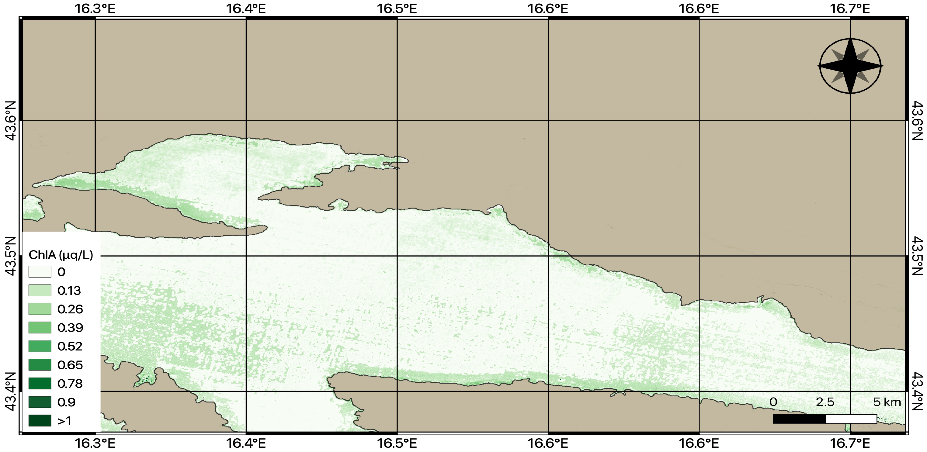
In order to further investigate the validity of the obtained formula, we observed the spatial distribution of the predicted Chl-a value for the whole water body of the study area. Estimated Formula (10) is applied to .tiff band images by using the raster calculator in the free and open-source GIS (Geographic Information System) software—QGIS [50]. Figure 7 shows mapped Chl-a in the Kaštela Bay and the Brač Channel using the newly proposed formula and Sentinel Level-2A satellite data from 30 September 2017. Higher concentration of Chl-a can be spotted at the coastline where the circulation of water is lower. The obtained map confirms our assumptions that Chl-a is higher in the nearby vicinity of the rivers Jadro and Cetina and along the coast.

Furthermore, in Figure 7, it is possible to see how the applied formula separates the land from the sea quite well, as well as the identification of other water surfaces and the concentrations of Chl-a in them (the example of the river Cetina).

Estimated formula assigns negative values to land and objects without chlorophyll, such as boats in the sea. We assume that this is the effect of vertical augmentation since the algorithm has learned that the features of the hard objects on land have low values of Chl-a. Of course, there are some pixels that are classified as Chl-a on land, but this is a model error that can be ignored.

3.1. Comparison with Other Methods for Chl-a Estimation

As we stressed in the related work section, many scientists have already developed different algorithms for the assessment of Chl-a concentration that are based on remote sensing. In this paper, we selected the two most common algorithms for implementation in order to check the performance of these algorithms over our data set, and to compare them to our algorithm. These two algorithms are as follows:

• Ocean color (OC3) algorithm, as proposed in [11], and coefficients adopted from the study in [12]. OC3 was implemented as a function to calculate the Chl-a value having the same band values as our algorithm. The resulting value was evaluated having in situ measurement as ground truth.
• Case-2 Regional/Coast Colour (C2RCC) algorithm [13]. We used the C2RCC processor provided in the SNAP processing toolbox from ESA. We collected the Sentinel-2 images from https://scihub.copernicus.eu/ (accessed on 12 October 2021) for several dates of the in situ measurements, processed the whole data set using C2RCC S2-MSI processor, and created a Chl-a map of the area. The processor used default parameters since other algorithms we compared did not use any external data or information. Predicted values of Chl-a concentration were further extracted only on the coordinates of measurement and compared with the in situ measurements.

The results of the evaluation are shown in

Table 7. Comparison of statistical evaluation indices of OC3, C2RCC, and our algorithm for predicting Chl-a concentration in respect to in situ measurements.

Algorithm	RMSE	${\mathit{R}}^2$
OC3 (Applied on the whole data set)	2.9255	−698.1315
C2RCC (Applied on selection of images)	1.6348	−6.9908
Our algorithm (Applied on test set)	0.2051	0.6599

. By comparing the shown values, we can conclude that according to both evaluation measures, our model results in better predictions compared with in situ measurement. This is not surprising, since our model is trained with in situ measurement data and tested on a portion of the data set that was not used for training but originated from the same source. However, what surprised us is that the correlation coefficient $R^2$ was negative for both OC3 and C2RCC. This shows that predictions of these two models are not correlated at all with in situ measurements. Negative $R^2$ score values means that the model does not follow the trend of the data. Both the OC3 and C2RCC algorithms predict the values of Chl-a that are not correlated at all with the in situ measurements. This means that Chl-a in our study area cannot be predicted with commonly used algorithms but needs a more suitable model, such as the one we developed in this research.

3.2. Qualitative Validation

In this section, we will demonstrate the usefulness of mapping Chl-a concentrations. First, we will show the resulting Chl-a map in case of occurrence of unwanted phenomenon related to Chl-a—Algae blooms. Algae blooms occur under certain weather conditions such as changes in temperature and higher rainfall in the spring; moreover, algal blooms are affected by an increased intake of nutrient salts of nitrogen and phosphorus that serve as food for phytoplankton [51].

Some algae can release toxins that negatively affect human health, but also lead to the extinction of fish and negative impacts on all seafood-dependent animals [52]. With algae blooms where the sea is bacteriologically clean, there is no danger to human health but it is an inconvenience to bathers during the summer season.

Detecting algae blooms is challenging, due to the different cell sizes and types of phytoplankton [53]. Chl-a can indicate a potential increase in algae, so maps of Chl-a concentrations calculated from satellite images can provide information on the possible spatial distribution of algae.

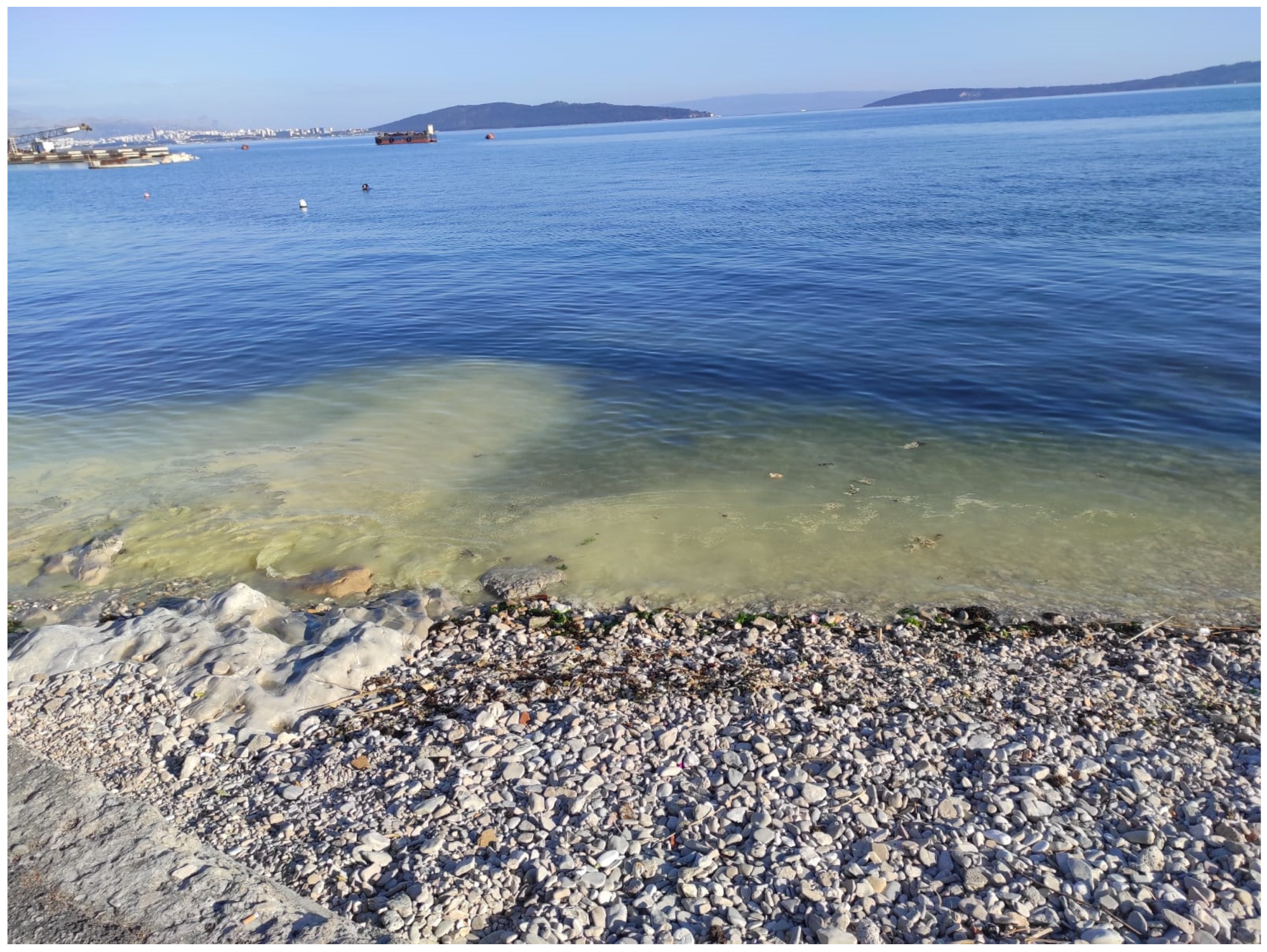
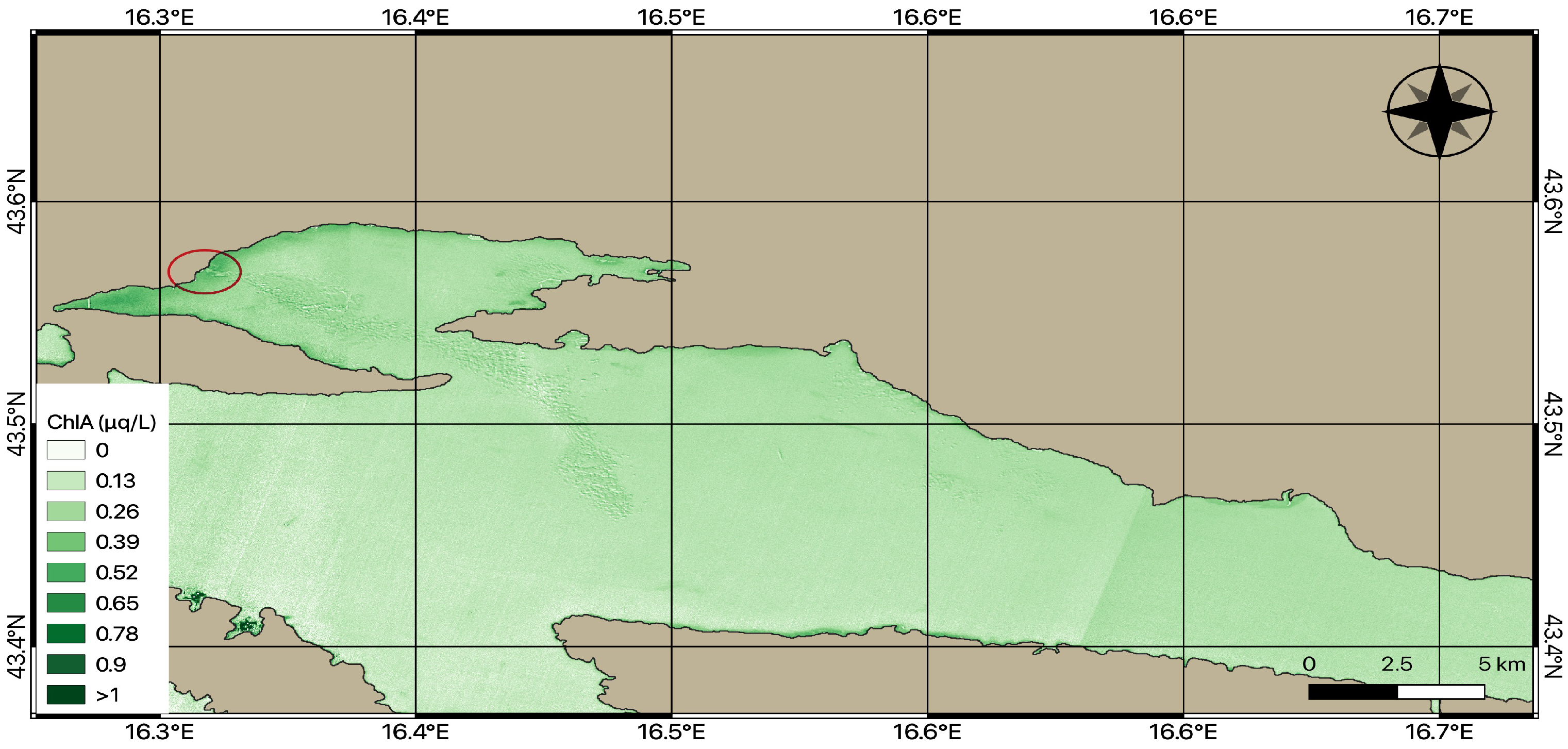
Figure 8 shows a photo of the beach in Kaštela Bay on 1 April 2021, where the algae blooms can be seen. This incident was reported in the media and discussed on social media. To see if our method for retrieving Chl-a can be used to detect changes in the sea during the algae blooms, we downloaded the first available satellite image taken on 2 April 2021 and applied Formula (10) on image bands (Figure 9).

In Figure 9, the same scale of Chl-a concentration range is applied as in Figure 7. The Sentinel Level-2A image (Figure 7) was taken in the period when there were no reported algae blooms in media for our study area. Based on the publicly available data published by the Ministry of Environmental Protection and Energy [54], which is a legal entity of the Republic of Croatia, in the summer and autumn months, the phytoplankton algae Dinophysis caudata from the Dinoflagellata group were recorded in relatively high abundance in almost all areas of the Adriatic sea. Dinophysis caudata algae produces toxic metabolites such as okadaic acid and DTX toxin. Based on these facts, the abundance of the algae population is potentially captured in the image (Figure 7), but we cannot claim this with certainty.

First, we can notice that the green color, which represents a higher concentration of Chl-a, is more pronounced at the time of algae blooms in Figure 9 compared with Figure 7 when there were no algae blooms in the sea. Comparing scenes with and without algae blooms can be the first indicator that changes are happening in the sea.

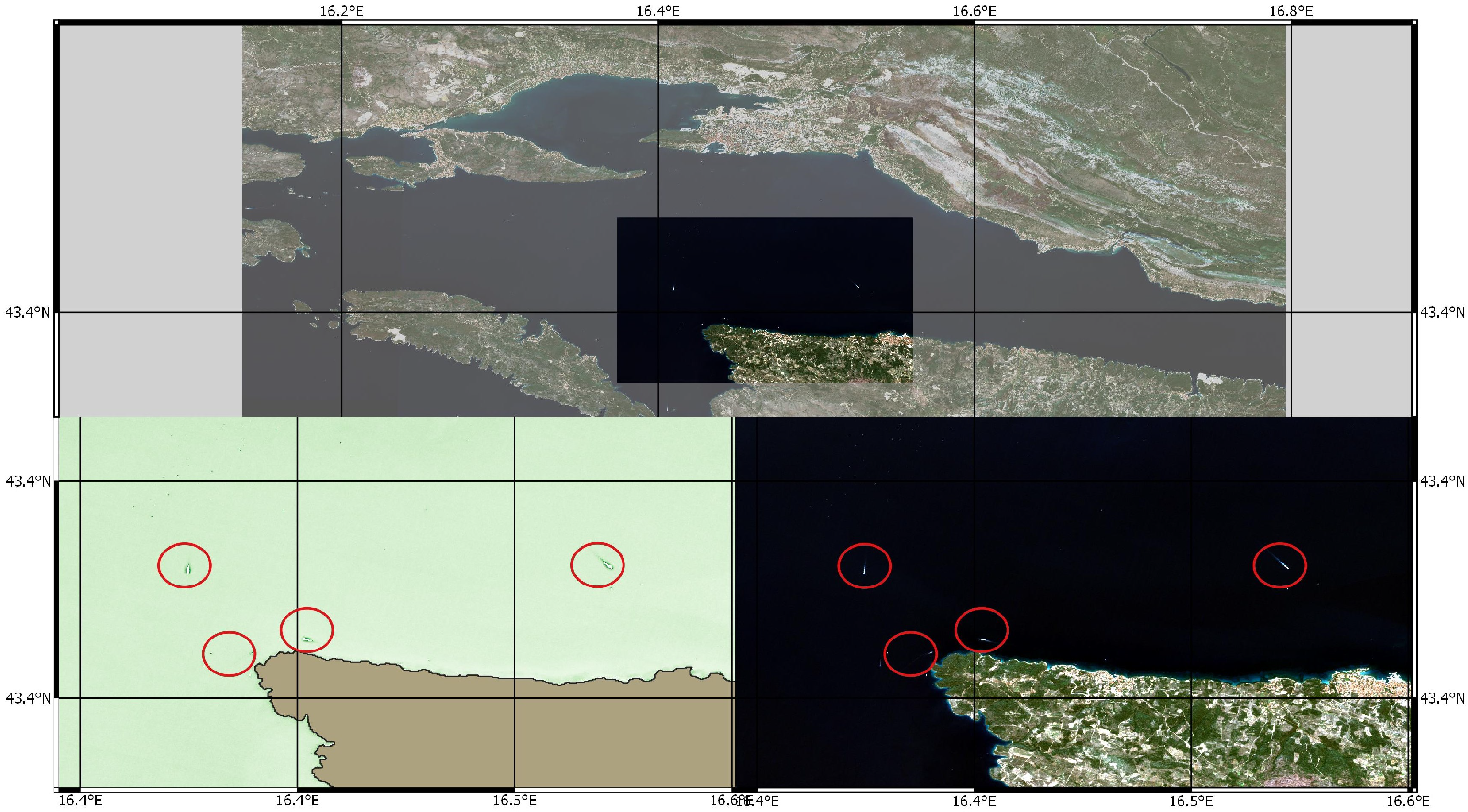
On Figure 9, we marked the location where the image (Figure 8) was taken with the ellipse. It is visible that the whole coast shows the highest concentration of Chl-a when the algae bloom incident occurred. This does not mean that any increase of Chl-a indicates the algae bloom incident but shows that our model detects the Chl-a of algae on the water surface. Nevertheless, our model also excludes objects in the sea such as boats, as shown in Figure 10. In this figure, we can clearly see boats in the sea near the shore at the time the satellite image was taken.

4. Conclusions and Future Work

This study describes a method for obtaining the Ridge Regression model applied to in situ and Sentinel Level-2A satellite data and discusses the obtained results. The data set is constructed by making feature augmentation and adding arbitrary points representing stations with zero concentration of Chl-a. The best results in the application of Ridge regression had a combination that included all of the transformed features of the bands, both for train ($R^2=0.685$ and $RMSE=0.2254$) and test data ($R^2=0.6599$ and $RMSE=0.2051$). Obtained coefficients of applied Ridge Regression model are used for the implementation of MLR formula in order to estimate and map Chl-a distribution in the Adriatic sea for the areas of Kaštela Bay and the Brač Channel situated in the Republic of Croatia. In the estimated formula for Chl-a prediction, bands B01, B02, B04, B05, B06, B8A, B11, and B12 in different transformations showed the best correlation with in situ Chl-a data. Predicted concentration of Chl-a is high at the coast and nearby rivers, which are areas usually classified as places with a high Chl-a trend.

One of the undesirable sea phenomena that can be unpleasant and dangerous for human and animal health is algae blooms. They can cause discomfort to bathers in the summer; so, it is useful to monitor and predict changes in the sea. We applied a formula for predicting Chl-a on Sentinel-2 images taken on the date of the incident of algae blooms that occurred in April 2021 in our study area. This showed larger deviations in Chl-a concentration during algae blooms, compared with when there was no algae bloom in this area. Thus, prediction of Chl-a concentration using remote sensing gives us the opportunity to monitor the water quality in an inexpensive way and gives us a broader picture of distribution of Chl-a.

Statistical evaluation of our algorithm shows that it is possible to find correlations of band values and transformations of those values with measured Chl-a concentration for oligotrophic waters with relatively small values of Chl-a concentration. Our model output is more correlated with measurement values than the prediction of OC3 and C2RCC algorithms.

In the future, in addition to chlorophyll, other optical parameters such as turbidity, total suspended matter (TSM), and colored dissolved organic matter (CDOM) can be used to predict water quality. Therefore, to improve the existing model, we could include the listed parameters in order to achieve higher accuracy for water quality prediction. Additionally, for better results, it is necessary to further enrich the data set for training and testing, so we plan to include data from other satellites in our future work, such as Sentinel-3 or Landsat-8. In this way, the data set will be enriched with measurements for which we excluded the data from the Sentinel-2 satellite.

References

1. Zemla, S.; Zemla, N.; Gelo, F. Factors Influencing Tourism Growth in Croatia. Tourism, Innovations and Entrepreneurship TIE 2019. p. 5. Available online: https://learning.stacksdiscovery.com/eds/detail?db=edb&an=149083081 (accessed on 12 October 2021).
2. Ha, N.T.T.; Thao, N.T.P.; Koike, K.; Nhuan, M.T. Selecting the Best Band Ratio to Estimate Chlorophyll-a Concentration in a Tropical Freshwater Lake Using Sentinel 2A Images from a Case Study of Lake Ba Be (Northern Vietnam). ISPRS Int. J. Geo-Inf. 2017, 6, 290. [Google Scholar] [CrossRef]
3. Matus Hernández, M.; Hernandez Saavedra, N.; Martinez Rincon, R. Predictive performance of regression models to estimate Chlorophyll—A concentration based on Landsat imagery. PLoS ONE 2018, 13, e0205682. [Google Scholar] [CrossRef] [PubMed] [Green Version]
4. Guo, Q.; Wu, X.; Bing, Q.; Pan, Y.; Wang, Z.; Fu, Y.; Wang, D.; Liu, J. Study on Retrieval of Chlorophyll-a Concentration Based on Landsat OLI Imagery in the Haihe River, China. Sustainability 2016, 8, 758. [Google Scholar] [CrossRef] [Green Version]
5. Sharaf El Din, E.; Zhang, Y. Estimation of both optical and nonoptical surface water quality parameters using Landsat 8 OLI imagery and statistical techniques. J. Appl. Remote Sens. 2017, 11, 046008. [Google Scholar] [CrossRef]
6. Senta, A.; Šerić, L. Remote sensing data driven bathing water quality assessment using sentinel-3. Indones. J. Electr. Eng. Comput. Sci. 2021, 21, 1634–1647. [Google Scholar] [CrossRef]
7. Fernanda, W.; Enner, A.; Thanan, R.; Luiz, R.; Nariane, B.; Nilton, I. Remote sensing of the chlorophyll-a based on OLI/Landsat-8 and MSI/Sentinel-2A (Barra Bonita reservoir, Brazil). Anais da Academia Brasileira de Ciências 2017, 90 (Suppl. 1), 1987–2000. [Google Scholar]
8. Potes, M.; Costa, M.J.; Salgado, R. Satellite remote sensing of water turbidity in Alqueva reservoir and implications on lake modelling. Hydrol. Earth Syst. Sci. 2012, 16, 1623–1633. [Google Scholar] [CrossRef] [Green Version]
9. Mao, Z.; Chen, J.; Pan, D.; Tao, B.; Zhu, Q. A regional remote sensing algorithm for total suspended matter in the East China Sea. Remote Sens. Environ. 2012, 124, 819–831. [Google Scholar] [CrossRef]
10. Shanmugam, P. New models for retrieving and partitioning the colored dissolved organic matter in the global ocean: Implications for remote sensing. Remote Sens. Environ. 2011, 115, 1501–1521. [Google Scholar] [CrossRef]
11. O’Reilly, J.E.; Werdell, P.J. Chlorophyll algorithms for ocean color sensors-OC4, OC5 & OC6. Remote Sens. Environ. 2019, 229, 32–47. [Google Scholar] [PubMed]
12. Pahlevan, N.; Smith, B.; Schalles, J.; Binding, C.; Cao, Z.; Ma, R.; Alikas, K.; Kangro, K.; Gurlin, D.; Hà, N.; et al. Seamless retrievals of chlorophyll-a from Sentinel-2 (MSI) and Sentinel-3 (OLCI) in inland and coastal waters: A machine-learning approach. Remote Sens. Environ. 2020, 240, 111604. [Google Scholar] [CrossRef]
13. Brockmann, C.; Doerffer, R.; Peters, M.; Kerstin, S.; Embacher, S.; Ruescas, A. Evolution of the C2RCC neural network for Sentinel 2 and 3 for the retrieval of ocean colour products in normal and extreme optically complex waters. Living Planet Symp. 2016, 740, 54. [Google Scholar]
14. ESA. SNAP—SentiNel Application Platform. 2021. Available online: http://step.esa.int/main/download/snap-download/ (accessed on 20 July 2021).
15. Katlane, R.; Dupouy, C.; El Kilani, B.; Berges, J.C. Estimation of chlorophyll and turbidity using sentinel 2A and EO1 data in Kneiss Archipelago Gulf of Gabes, Tunisia. Int. J. Geosci. 2020, 11, 708. [Google Scholar] [CrossRef]
16. Page, B.P.; Kumar, A.; Mishra, D.R. A novel cross-satellite based assessment of the spatio-temporal development of a cyanobacterial harmful algal bloom. Int. J. Appl. Earth Obs. Geoinf. 2018, 66, 69–81. [Google Scholar] [CrossRef]
17. Kuhn, C.; de Matos Valerio, A.; Ward, N.; Loken, L.; Sawakuchi, H.O.; Kampel, M.; Richey, J.; Stadler, P.; Crawford, J.; Striegl, R.; et al. Performance of Landsat-8 and Sentinel-2 surface reflectance products for river remote sensing retrievals of chlorophyll-a and turbidity. Remote Sens. Environ. 2019, 224, 104–118. [Google Scholar] [CrossRef] [Green Version]
18. Bergsma, E.W.; Almar, R. Coastal coverage of ESA’ Sentinel 2 mission. Adv. Space Res. 2020, 65, 2636–2644. [Google Scholar] [CrossRef]
19. Nazeer, M.; Nichol, J.E. Development and application of a remote sensing-based Chlorophyll-a concentration prediction model for complex coastal waters of Hong Kong. J. Hydrol. 2016, 532, 80–89. [Google Scholar] [CrossRef]
20. Lee, Z.; Shang, S.; Qi, L.; Yan, J.; Lin, G. A semi-analytical scheme to estimate Secchi-disk depth from Landsat-8 measurements. Remote Sens. Environ. 2016, 177, 101–106. [Google Scholar] [CrossRef]
21. Caballero, I.; Fernández, R.; Escalante, O.M.; Mamán, L.; Navarro, G. New capabilities of Sentinel-2A/B satellites combined with in situ data for monitoring small harmful algal blooms in complex coastal waters. Sci. Rep. 2020, 10, 8743. [Google Scholar] [CrossRef]
22. He, X.; Pan, D.; Mao, Z. Water-Transparency (Secchi Depth) Monitoring in the China Sea with the SeaWiFS Satellite Sensor. Remote Sens. Agric. Ecosyst. Hydrol. 2004, 5568, 112–122. [Google Scholar] [CrossRef]
23. Barale, V.; Jaquet, J.M.; Ndiaye, M. Algal blooming patterns and anomalies in the Mediterranean Sea as derived from the SeaWiFS data set (1998–2003). Remote Sens. Environ. 2008, 112, 3300–3313. [Google Scholar] [CrossRef]
24. Politi, E.; Prairie, Y.T. The potential of Earth Observation in modelling nutrient loading and water quality in lakes of southern Québec, Canada. Aquat. Sci. 2018, 80, 8. [Google Scholar] [CrossRef]
25. Ouma, Y.; Noor, K.; Herbert, K. Modelling Reservoir Chlorophyll-a, TSS, and Turbidity Using Sentinel-2A MSI and Landsat-8 OLI Satellite Sensors with Empirical Multivariate Regression. J. Sens. 2020, 2020, 8858408. [Google Scholar] [CrossRef]
26. Ouma, Y.O.; Waga, J.; Okech, M.; Lavisa, O.; Mbuthia, D. Estimation of reservoir bio-optical water quality parameters using smartphone sensor apps and Landsat ETM+: Review and comparative experimental results. J. Sens. 2018, 2018, 3490757. [Google Scholar] [CrossRef]
27. Patra, P.; Dubey, S.; Trivedi, R.; Sahu, S.; Rout, S. Estimation of Chlorophyll-a Concentration and Trophic States for an Inland Lake from Landsat 8 OLI Data: A Case of Nalban Lake of East Kolkata Wetland, India. Sciprints 2016. [Google Scholar] [CrossRef] [Green Version]
28. Hansen, C.; Williams, G.; Adjei, Z. Long-Term Application of Remote Sensing Chlorophyll Detection Models: Jordanelle Reservoir Case Study. Nat. Resour. 2015, 6, 123–129. [Google Scholar] [CrossRef] [Green Version]
29. Shih, S.F.; Gervin, J.C. Ridge Regression Techniques Applied to Landsat Investigation of Water Quality in Lake Okeechobee. JAWRA J. Am. Water Resour. Assoc. 1980, 16, 790–796. [Google Scholar] [CrossRef]
30. Hrvatska enciklopedija, mrežno izdanje. Kaštelanski zaljev. 2021. Available online: http://www.enciklopedija.hr/Natuknica.aspx?ID=30791 (accessed on 12 October 2021).
31. Hrvatska enciklopedija, mrežno izdanje. Brački kanal. 2021. Available online: http://www.enciklopedija.hr/Natuknica.aspx?ID=9141 (accessed on 12 October 2021).
32. Vela, S. Structure of the Bycatch and Discard of the Bottom Trawling Fisheries in the Middle Adriatic Channels. Ph.D. Thesis, Institute of Oceanography and Fisheries, Split, Croatia, 2011. [Google Scholar]
33. Hrvatske Vode. d.o.o. Metodologija Uzorkovanja, Laboratorijskih Analiza I Određivanja Omjera EkološKE Kakvoć E BiološKih Elemenata KakvoćE. 2015. Available online: https://www.voda.hr/sites/default/files/dokumenti/metodologija_uzorkovanja_laboratorijskih_analiza_i_odredivanja_omjera_ekoloske_kakvoce_bioloskih_elemenata_kakvoce_1.pdf (accessed on 12 October 2021).
34. Du, Y.; Zhang, Y.; Ling, F.; Wang, Q.; Li, W.; Li, X. Water Bodies’ Mapping from Sentinel-2 Imagery with Modified Normalized Difference Water Index at 10-m Spatial Resolution Produced by Sharpening the SWIR Band. Remote Sens. 2016, 8, 354. [Google Scholar] [CrossRef] [Green Version]
35. Sola, I.; García-Martín, A.; Sandonís-Pozo, L.; Álvarez Mozos, J.; Pérez-Cabello, F.; González-Audícana, M.; Montorio Llovería, R. Assessment of atmospheric correction methods for Sentinel-2 images in Mediterranean landscapes. Int. J. Appl. Earth Obs. Geoinf. 2018, 73, 63–76. [Google Scholar] [CrossRef]
36. Sinergise Ltd. Modified Copernicus Sentinel Data (2017–2019)/Sentinel Hub. Available online: https://apps.sentinel-hub.com/eo-browser/ (accessed on 22 April 2021).
37. Main-Knorn, M.; Pflug, B.; Louis, J.; Debaecker, V.; Müller-Wilm, U.; Gascon, F. Sen2Cor for Sentinel-2. In Proceedings of the Image and Signal Processing for Remote Sensing XXIII, Warsaw, Poland, 11–14 September 2017; Volume 10427, pp. 37–48. Available online: https://www.spiedigitallibrary.org/conference-proceedings-of-spie/10427/2278218/Sen2Cor-for-Sentinel-2/10.1117/12.2278218.short (accessed on 12 October 2021). [CrossRef] [Green Version]
38. Tranmer, M.; Elliot, M. Multiple Linear Regression; The Cathie Marsh Centre for Census and Survey Research (CCSR), 2008; Volume 5, pp. 1–5. Available online: http://hummedia.manchester.ac.uk/institutes/cmist/archive-publications/working-papers/2020/multiple-linear-regression.pdf (accessed on 12 October 2021).
39. Marill, K.A. Advanced statistics: Linear regression, part II: Multiple linear regression. Acad. Emerg. Med. 2004, 11, 94–102. [Google Scholar] [CrossRef] [PubMed]
40. Kim, S.W.; Jung, D.; Choung, Y.J. Development of a Multiple Linear Regression Model for Meteorological Drought Index Estimation Based on Landsat Satellite Imagery. Water 2020, 12, 3393. [Google Scholar] [CrossRef]
41. Saleh, A.M.E.; Arashi, M.; Kibria, B.G. Theory of Ridge Regression Estimation with Applications; John Wiley & Sons: Hoboken, NJ, USA, 2019; Volume 285. [Google Scholar]
42. Chatterjee, S.; Hadi, A.S. Regression Analysis by Example; John Wiley & Sons: Hoboken, NJ, USA, 2015. [Google Scholar]
43. Hoerl, A.E.; Kennard, R.W. Ridge regression: Biased estimation for nonorthogonal problems. Technometrics 1970, 12, 55–67. [Google Scholar] [CrossRef]
44. Mansouri, E.; Feizi, F.; Jafari Rad, A.; Arian, M. Remote-sensing data processing with the multivariate regression analysis method for iron mineral resource potential mapping: A case study in the Sarvian area, central Iran. Solid Earth 2018, 9, 373–384. [Google Scholar] [CrossRef] [Green Version]
45. Sara, U.; Akter, M.; Uddin, M.S. Image quality assessment through FSIM, SSIM, MSE and PSNR—A comparative study. J. Comput. Commun. 2019, 7, 8–18. [Google Scholar] [CrossRef] [Green Version]
46. Qin, P.; Simis, S.; Tilstone, G. Radiometric validation of atmospheric correction for MERIS in the Baltic Sea based on continuous observations from ships and AERONET-OC. Remote Sens. Environ. 2017, 200, 263–280. [Google Scholar] [CrossRef] [Green Version]
47. DeVries, T.; Taylor, G.W. Dataset augmentation in feature space. arXiv 2017, arXiv:1702.05538. [Google Scholar]
48. Garson, G.D. Testing Statistical Assumptions; Statistical Associates Publishing: Asheboro, NC, USA, 2012. [Google Scholar]
49. Grendaitė, D.; Stonevicius, E.; Karosienė, J.; Savadova-Ratkus, K.; Kasperovičienė, J. Chlorophyll-a concentration retrieval in eutrophic lakes in Lithuania from Sentinel-2 data. Geol.Geogr. 2018, 4. [Google Scholar] [CrossRef]
50. QGIS Development Team. QGIS Geographic Information System. 2021. Available online: https://www.qgis.org (accessed on 12 October 2021).
51. Xie, Y.; Tilstone, G.H.; Widdicombe, C.; Woodward, E.M.S.; Harris, C.; Barnes, M.K. Effect of increases in temperature and nutrients on phytoplankton community structure and photosynthesis in the western English Channel. Mar. Ecol. Prog. Ser. 2015, 519, 61–73. [Google Scholar] [CrossRef] [Green Version]
52. Ferrante, M.; Gea, O.C.; Fiore, M.; Rapisarda, V.; Ledda, C. Harmful Algal Blooms in the Mediterranean Sea: Effects on Human Health. EuroMediterr. Biomed. J. 2013, 8, 25–34. [Google Scholar] [CrossRef]
53. Shen, F.; Tang, R.; Sun, X.; Liu, D. Simple methods for satellite identification of algal blooms and species using 10-year time series data from the East China Sea. Remote Sens. Environ. 2019, 235, 111484. [Google Scholar] [CrossRef]
54. Živana, N.G. Fitoplanktonske alge u Prijelaznim i Priobalnim Vodama i moru WEU14 (2019. godina). Ministarstvo Zaštite Okoliša i Energetike. Available online: http://baltazar.izor.hr/azopub/indikatori_podaci_sel_detalji2?p_ind_br=2B13&p_godina=2019 (accessed on 22 August 2021).
Figure 1. Map of the geographical location of the study area (Kaštela Bay and The Brač Channel) in the context of Europe and the Republic of Croatia.
Electronics 10 03004 g001
Figure 2. Map of in situ measuring stations distributed over the study area.
Electronics 10 03004 g002
Figure 3. Data set construction.
Electronics 10 03004 g003
Figure 4. Distribution of time differences between satellite image and in situ measurement expressed in days.
Electronics 10 03004 g004
Figure 5. Illustration of two axes of augmentation performed on original data set.
Electronics 10 03004 g005
Figure 6. Prediction error plot shows the relationship between in situ and predicted Chlorophyll-a values on train (left) and test (right) data.
Electronics 10 03004 g006
Figure 7. Map of the predicted Chlorophyll-a and its distribution over the Kaštela Bay and the Brač Channel on 30 September 2017.
Electronics 10 03004 g007
Figure 8. Algae Blooms in Kaštela Bay on 1 April 2021.
Electronics 10 03004 g008
Figure 9. Map of the predicted Chlorophyll-a and its distribution over Kaštela Bay and the Brač Channel on 2 April 2021—algae blooms occurs.
Electronics 10 03004 g009
Figure 10. Example of excluded boats from Chl-a calculation in the Brač Channel on 30 September 2017.
Electronics 10 03004 g010