Comparison of Deep Neural Network Models and Effectiveness of EMG Signal Feature Value for Estimating Dorsiflexion

Abstract

Robotic ankle–foot orthoses (AFO) are often used for gait rehabilitation. Our research focuses on the design and development of a robotic AFO with minimum number of sensor inputs. However, this leads to degradation of gait estimation accuracy. To prevent degradation of accuracy, we compared a few neural network models in order to determine the best network when only two input channels are being used. Further, the EMG signal feature value of average rate of change was used as input. LSTM showed the highest accuracy. However, MLP with a small number of hidden layers showed results similar to LSTM. Moreover, the accuracy for all models, with the exception of LSTM for one subject (SD), increased with the addition of feature value (average rate of change) as input. In conclusion, time-series networks work best with a small number of sensor inputs. However, depending on the optimizer being used, even a simple network can outrun a deep learning network. Furthermore, our results show that applying EMG signal feature value as an input tends to increase the estimation accuracy of the network.

1. Introduction

The foot drop is defined as the inability to properly perform dorsiflexion movement at the ankle joint as the foot cannot clear the ground during the swing phase of the gait cycle [1]. More precisely, a weakness or failure in functioning of the tibialis anterior (TA) causes restricted movement, such as reduced gait speed and increased risk of falling [2,3]. Foot drop is usually caused by strokes. Strokes lead to damage of the motor cortex or corticospinal tract and often result in contralateral hemiplegia [3]. Studies have shown that 70–80% of stroke survivors will recover the ability to independently walk short distances without assistance of another person [4]. However, only 50% of survivors can achieve limited community ambulation status or better [4]. The chances of a stroke survivor regaining independent walking are approximately 60% with the help of rehabilitation [5].

AFOs are usually applied during gait rehabilitation [4,5,6]. AFOs enhance the patient’s walking function by providing stability and support during stance or foot clearance at the swing phase of the gait cycle [4]. The most common type of AFO is the rigid AFO, which has a highly stable design that is capable of holding the ankle in a rigid position with limited movement in all planes [4]. Compared to rigid AFOs, articulate AFOs are more flexible because of the articulated joints. These AFOs are designed to provide dorsiflexion support during the swing phase and still allow some ankle movement during the stance phase [4]. AFOs are often made of lightweight, rigid plastic materials that brace the ankle joint to prevent any undesirable movements. However, most AFOs limit some ankle movements of the paretic side and may not allow the user to completely regain strength of the lower limb [1]. AFOs with articulated joints have the least limitations to basic ankle movements because of its functional capacity to rotate 360° angle. However, AFOs with articulated joint cannot control the ankle position and motion by themselves [7]. This can result in gait abnormalities and inability to achieve full potential of the ankle motion [1]. Because of the problems stated, robotic devices are being developed [6].

Robotic AFO devices lock the ankle angle, thereby preventing foot drag in the swing phase and providing large resistive dorsiflexion torque in the loading stance phase [6]. The use of additional components such as sensors in the development of articulated joint robotic AFO can simulate the gait of able-bodied subjects for patient training purposes [7]. Further, recent research has proven that patients with foot drop can regain the control of their ankle motion with the use of robotic AFOs [4,5,6,8].

In this study, we focused on AFOs that use surface electromyography (sEMG) sensors as input channels [9]. Recent studies have shown that sEMG is often used during rehabilitation because of its noninvasiveness. It does not involve any pain and discomfort and can be easily applied to the skin [10,11,12]. However, each person has different sEMG patterns. Even in the same person, different environments can affect the sEMG signal pattern.

When considering the variability of sEMG signals, various parts of the leg’s sEMG, from thigh to ankle, are taken into account to estimate a person’s gait motion. As mentioned previously, the main problem with foot drop is the failure to perform dorsiflexion during the swing phase of the gait cycle, which leads to increased risk of falling [2]. On the other hand, if the dorsiflexion operation is performed accurately during the gait cycle, the risk of falling can be reduced.

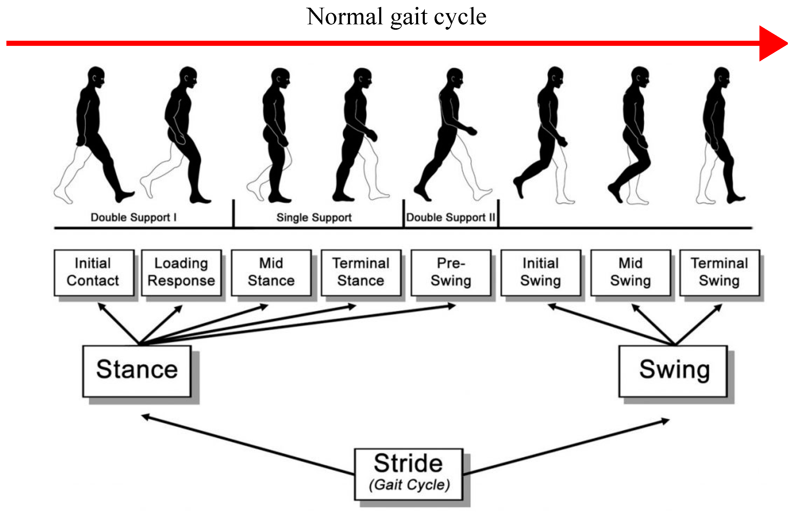
Unfortunately, lower limb sEMG can easily be affected by body gravity and muscle jitter. This can be considered as one of the main reasons why many studies have been inconclusive [9]. In this study, we focused on using minimum number of sEMG input channels for ankle movement estimation. We focused on applying machine learning (ML) and deep neural networks (DNNs) to estimate the toe position during the gait cycle. Models such as support vector machine (SVM) classifier are often used to classify the motion of a certain movement. In this research, we mainly focused on estimating the dorsiflexion motion, meaning a classifier was unnecessary. To be precise, we aimed to estimate the acceleration of the toe motion during the gait cycle (Figure 1).

The acceleration value of the toe motion can be used to detect the position of the toe during the swing phase. Therefore, it can be taken as the primary source of data for the dorsiflexion motion. At the early stage of our research, tests were conducted using one sEMG sensor on the ankle area. Unfortunately, one sEMG signal was not able to estimate the dorsiflexion motion during the gait cycle. This is because sEMG signals are nonlinear, and we found that sEMG signals have almost no correlation with the acceleration of the toe motion during the gait cycle. Without any correlation between the two data sets, estimating the acceleration of the toe motion during the gait cycle through DNNs was considered impossible. We also considered the EMG signal feature value during the gait cycle as input channels to provide more information for the training process.

The main purpose of this research was to investigate the best neural network model that can estimate the acceleration of the toe motion during the gait cycle with the least number of sEMG sensors and to examine the effects of applying EMG signal feature values as inputs.

In this paper, we talk about the applicability of different neural network models. The models that we focused on are as follows:

• Adaptive neuro-fuzzy inference system (ANFIS).
• Multilayer perceptron (MLP) consisting of 4 layers, where the first layer is the input layer; the second and third layers are hidden layers with 5 and 3 neurons, respectively; and the fifth layer is the output layer.
• Multilayer perceptron with deeper hidden layers, with 7 layers consisting of 128, 64, 32, 16, and 8 neurons, respectively.
• Long short-term memory deep neural network (LSTM).

Each model is explained separately in this paper. Furthermore, we considered the feature values of sEMG signals as input channels. In previous studies, we discovered that the feature values can be used to improve estimation accuracy during the training process [11,12]. A common problem that occurs when using fewer sensor inputs is insufficient gait information during the gait cycle, which affects the estimation accuracy [7]. In order to avoid this problem, we decided to apply the following approaches in our research. To confirm our theory, we conducted several experiments based on these methods.

• The first experiment used training models with only two sensors without feature values as input channels.
• The second experiment used training models with two sensors and additional feature values as input channels [13,14].

Both results were compared. Based on previous studies, it was predicted that the neural network with deep learning applied would have higher accuracy compared to the artificial neural network. We also predicted that the LSTM network would result in the highest accuracy compared to other models due to its features. Moreover, by adding feature values as input channels, the estimation accuracy of the acceleration of the toe motion during the gait cycle would increase despite the use of minimum number of sEMG sensors.

2. Methods

2.1. Participants

In this experiment, a total of 3 test subjects, all men aged 20, were recruited. The 3 subjects were in good health condition. Subjects who had any history of musculoskeletal injuries, neurological disorder, and age-related health issues were excluded. During the experiment, data were collected only on the right foot as all participants were right-handed. As an experiment with 3 test subjects is comparatively low, several tests were conducted on a single test subject to acquire a variety of data sets. All methods were performed in accordance with the relevant guidelines and regulations. Written consent was also obtained from the 3 participants, and no violation of human rights was reported.

2.2. Device

For data acquisition, two sEMG wireless sensors from Delsys Trigno by Delsys Inc (Natick, MA, USA) were used. These Trigno Avanti sensors combine EMG and increase IMU performance. Therefore, they can be used to measure sEMG signals, movement acceleration, gyroscope, and magnitude measurement. In this experiment, the EMG and acceleration sensors were used to collect sEMG signals and motion data during the gait cycle.

The sensor’s resolution is 16 bits, its mass is 14 g, and it is 27 × 37 × 13 mm in size. It is supported on a low-noise, high-fidelity sensing circuit for detecting EMG signals from the surface of the skin when the muscle is contracted. The sensor also has an environmentally sealed enclosure that protects electronics from ingress of liquids. Furthermore, the average accuracy of the Delsys sensor is 95% [15].

The data mentioned above were collected through the computer software provided by Delsys Inc (Natick, MA, USA). (EMGworks). After performing the experiments, the acquired data were analyzed using Microsoft Excel (by Microsoft Corporation founded in Albuquerque, NM, USA) and Python programming language.

2.3. Environment

Experiments were conducted at Prof. Tamura’s Integrated Technology Lab, Department of Environmental Robotics, Faculty of Engineering, University of Miyazaki.

2.4. Data Collection

Experiments consisted of four sessions. For all sessions, the participants were requested to perform a walking gesture for a fixed distance of 70 m. Gait sEMG signals are highly sensitive, resulting in diverse signals based on the subject’s condition. Tests were conducted 4 times for each subject in order to provide variations of raw gait sEMG signals. The participants were asked to walk at a normal walking speed (average speed of 100 bpm). Sensors were placed on the right foot of each test subject as mentioned earlier, and the right foot gait cycle data were collected and observed in each session. The session was initiated at 0 m, starting with the right foot and ending at the preset stopping point (70 m) with the right foot. This continued for 4 sessions with 5 s intervals between each walking session. Therefore, fatigue could be different between the first session and the last session.

The experiment was repeated as soon as the fourth session was over. In order to ensure data were not interrupted by any obstacle surrounding the ankle and toe area during the gait session, test subjects were instructed to stay barefoot. The area around the ankle and toe was clean and sanitized beforehand. The two EMG sensors were placed around the ankle joint to measure muscle activities during the gait session, while one accelerometer was placed near the toe area.

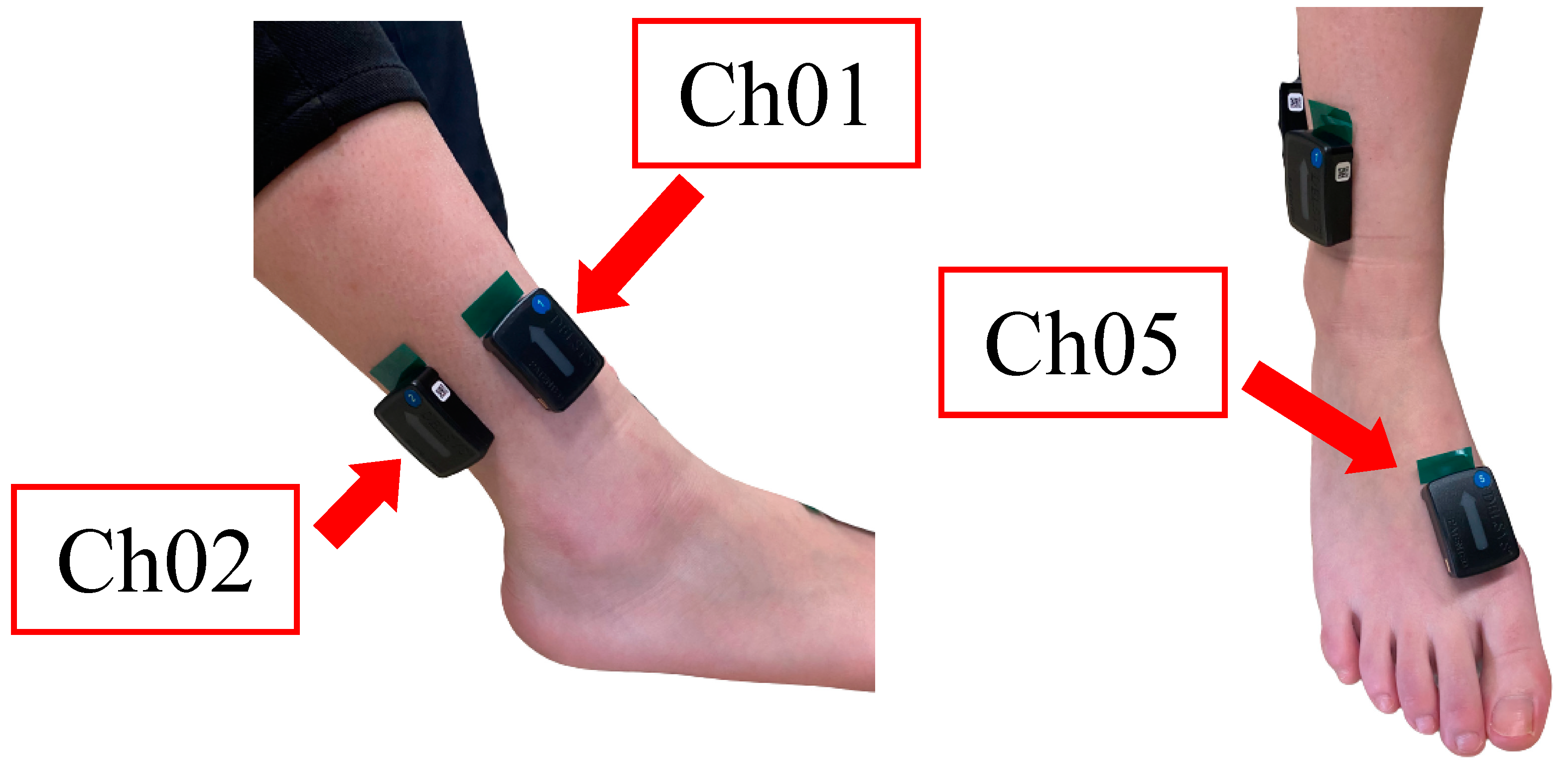
Dorsiflexion requires the TA, extensor digitorum longus (EDL), extensor hallucis longus (EHL), and peroneus tertius muscles [16]. In this experiment, we focused only on the muscles surrounding the ankle area as our aim was to develop a reliable robotic AFO for the future. Therefore, as the muscle nearest to the ankle, the EDL muscle was taken into consideration. Sensor 1 was placed on the surface where the EDL muscle is located (Figure 2) in order to collect the sEMG signal of dorsiflexion activities during the swing phase of the walking session. While Sensor 1 acquired data during the swing phase of the gait cycle, Sensor 2 was set to collect data during the stance phase of the gait cycle. In this case, the soleus muscle, which is nearest to the ankle, would transmit EMG signals during the stance phase. Thus, Sensor 2 was placed on the surface where the soleus muscle is located (Figure 2).

The accelerometer was placed on the dorsum of the foot between the first and second metatarsals in order to collect data on acceleration of the toe motion during the gait cycle (Figure 2). As we generally know, dorsiflexion occurs on the sagittal plane, which is the anatomical vertical plane that divides the body into left side and right side [17]. Therefore, y-axis data of the acceleration sensor alone are enough to estimate acceleration of the dorsiflexion motion during the gait cycle.

In this case, the root mean square error (RMSE), mean square error (MSE), and R-squared value were taken into account as evaluation methods.

Root mean square error (RMSE):

$$RMSE=\sqrt{{\displaystyle \sum }_{i=1}^n\frac{{\left({\widehat{y}}_i-y_i\right)}^2}{n}}$$

Mean square error (MSE):

$$MSE={\displaystyle \sum }_{i=1}^n\frac{{\left({\widehat{y}}_i-y_i\right)}^2}{n}$$

R-squared:

$$R^2=1-\frac{S{S}_{RES}}{S{S}_{TOT}}=1-\frac{{{\displaystyle \sum }}_i{\left(y_i-{\widehat{y}}_i\right)}^2}{{{\displaystyle \sum }}_i{\left(y_i-\overline{y}\right)}^2}$$

where ${\widehat{y}}_i$ is the estimated output value, and $y_i$ is the target output value. RMSE, MSE, and R-squared value varies from 0 to 1. For RMSE and MSE, 0 refers to 0% error, while 1 refers to 100% error. For R-squared value, 0 refers to 0% linear correlation, while 1 refers to 100% linear correlation. Training was performed 10 time for each participant, and the mean and standard deviation of each evaluation were recorded.

2.5. Data Filtering

Data collected by Trigno Avanti sensors have their own default settings [15]. Considering the difference in sampling rate of the EMG and acceleration data, it is necessary to adopt a method of resampling that ensures both data sets have the same sample rate.

Furthermore, the acquired data sets need to undergo a sequence of operations, such as data processing, filtering, rectification, and smoothing. Such processes were performed using a Python program.

Because EMG signals possess both negative and positive values, if we try to calculate an average or mean EMG, the negative and positive values will cancel out. To address this issue, the following three processing methods were implemented.

• Removing the mean value from the signal.
• Filtering the signal.
• Rectifying the signal.

Removing the mean value brings the whole signal down so that the mean is located at 0 point. The Delsys Trigno Avanti EMG sensor has a bandwidth of 20–450 Hz, which is the range of an EMG signal (

Table 1. The sampling rate of EMG and ACC signal and their respective bandwidth.

Data Type	Sampling Rate	Bandwidth
EMG	1926 sa/s	20–450 Hz
ACC	148 sa/s	24–470 Hz

). However, just to be sure, digital filter with a high pass of 20 Hz and a low pass of 450 Hz was applied. Furthermore, in order to prevent the negative and positive values from canceling out, the filtered signal was rectified as a third step.

Scientists investigating muscle force and muscle activity often use a low-pass filter to capture the shape or “envelope” of the EMG signal as it is considered a better reflect force generated by a muscle. Therefore, we used this method to smoothen the signal by applying another low-pass filter (for the EMG envelope) with a low pass of 10 Hz.

For the acceleration data sets, direction is an important factor to determine the position of the toe motion during gait, especially during the swing phase. Thus, we only conducted the smoothening process. We set the low-pass filter (for the ACC envelope) to 10 Hz. The EMG data sets were normalized to the amplitude value of acceleration data as it was the maximum amplitude being recorded. The data sets were then saved in a Microsoft Excel file for training purposes. Such data sets need to be divided separately for the purposes of training, validation, and testing. Based on that, 60% of EMG data was used for training, 20% was used for validation, and the balance 20% was used for testing.

2.6. Neural Network Models

2.6.1. ANFIS

Adaptive neuro-fuzzy inference system (ANFIS) is a combination of artificial neural network (ANN) and the fuzzy inference system [18,19,20]. In this study, 2 input and 1 output channels were provided.

2.6.2. Multilayer Perceptron (MLP)

Multilayer Perceptron (MLP) was used in this research. In MLP, the number of neuron in the input and output layers depends on the applied problem, while the number of neuron in the hidden layer is undecided and can be changed through trial and error [21]. Upon completing the training process, the MLP model would be capable of calculating and estimating the output values of any given input [22]. In this research, two MLP-based neural network models were used.

• MLP (MLP-s)
  This model was built using the MATLAB (develop by MathWorks) neural network tool (nntool). The MLP-s model has 4 layers consisting of 1 input layer, 2 hidden layers, and 1 output layer, with each layer containing 2, 5, 3, and 1 neurons, respectively. Sigmoid function was applied as the activation function. Sigmoid function is very commonly used as it is a nonlinear function [23] that transforms the value in the range of 0 to 1. For the optimizer, we applied the algorithm that was provided by MATLAB, which was the Levenberg–Marquardt (LM) algorithm. This algorithm is widely used and outperforms simple gradient descent (GD) and other conjugate gradient methods [24].

• MLP with deep hidden layers (MLP-d)
  This model was built using Keras, a library that provides highly powerful and abstract building blocks to build deep learning networks. This model has deep hidden layers consisting of 7 layers, namely 1 input layer, 5 hidden layers, and 1 output layer, with each layer containing 2, 128, 64, 32, 16, 8, and 1 neurons, respectively. The deep neural network (DNN) contains multiple nonlinear hidden layers, thus making it easy for them to learn a very complicated relationship between inputs and outputs. However, a majority of these complicated relationships are the result of sampling noises, which exist in training sets but not in the real test data. This leads to overfitting of the model [25]. A method called dropouts was applied between layers to prevent the model from overfitting [25]. Dropouts prevent overfitting and provide an efficient way of approximately combining an exponential number of different neural network architectures [25]. The activation function applied to this model was rectified liner unit (ReLu) and linear. The advantage of using ReLu function is that all the neurons are not activated at the same time, meaning neuron will be deactivated only when the output of linear transformation is 0 [23]. We only applied the linear function to the output layer of the model. As for the optimizer, the Keras library provides a lot of choice. We chose Adam, a method for efficient stochastic optimization that only requires first-order gradients with little memory requirement. The method computes individual adaptive learning rates for different parameters from estimates of first and second moments of the gradients [26].

2.6.3. Long Short-Term Memory Network with Deep Hidden Layers (LSTM)

Recurrent network (RNN) is a model with loops in the hidden layers, which allows the model to take a sequence of samples as input and find time relationships between them. However, RNN is weak in terms of learning in a long-term relationship [27]. Long short-term memory (LSTM) networks can solve this issue by adding parameters to the hidden node loops. These parameters have the function to remember inputs for a long time [28]. LSTM networks is proven to be more effective than RNN, especially when they have several layers for each time step [27]. Therefore, we used the LSTM network instead of RNN. Like MLP-d, this model is also built using the Keras library. The LSTM model consists of 7 layers, namely 1 input layer, 5 hidden layers, and 1 output layer, with each layer containing 2, 128, 64, 32, 16, 8, and 1 neurons, respectively. LSTM networks need time step data, which leads to the input data becoming a 3D-shaped data set consisting of samples, timesteps, and features. Samples are the values inside a data set. Time steps are the time sequence of 1 sample. In this research, we set it to be 30 timesteps in a sample. Features are the number of inputs. In this case, it was 2 features. Thus, the input shape for this model was (none, 30, 2), where “none” is the number of values in the output layer. Similar to MLP-d, we applied ReLu and linear functions as the model’s activation functions. Linear function was only applied to the output layer because it is a not a nonlinear function. As for the optimizer, we applied the Adam optimizer.

2.7. Feature Values: Average Rate of Change (AROC)

In this study, we proposed a method that considers the feature values of an EMG signal as input channel. The feature value we used was the average rate of change (AROC) between the current EMG signal and its past EMG signals.

The AROC equation is defined as follows:

$$AROC=\frac{1}{N}{{\displaystyle \sum }}_{x=0}^{N-1}\left(f\left(N+x\right)-f\left(x+1\right)\right)$$

(1)

where x is the sEMG signals collected by the two sensors, and N is the current sEMG value in a data set. We carried out testing with N values of 10, 50, 100, and 200 and found that N = 100 estimated the best output value. With the addition of AROC, all models except ANFIS consisted of 4 neurons instead of 2 neurons in their input layer. The two neurons processed the sEMG data set collected by the two EMG sensors and the AROC data of each sEMG data set.

3. Results

Table 2. RMSEs, MSEs, and R-squared values for ANFIS, MLP-s, MLP-d, and LSTM for all test subjects (SD, RE, and MS).

		ANFIS			MLP-s			MLP-d			LSTM
		RMSE	MSE	${\mathit{R}}^2$	RMSE	MSE	${\mathit{R}}^2$	RMSE	MSE	${\mathit{R}}^2$	RMSE	MSE	${\mathit{R}}^2$
SD	Mean	0.308	0.095	0.238	0.241	0.058	0.395	0.264	0.069	0.384	0.243	0.059	0.502
	STD	0.018	0.011	0.008	0.009	0.004	0.012	0.002	0.001	0.010	0.007	0.003	0.033
RE	Mean	0.247	0.061	0.027	0.172	0.030	0.230	0.176	0.031	0.214	0.172	0.030	0.292
	STD	0.027	0.013	0.018	0.004	0.001	0.014	0.001	0.001	0.008	0.007	0.002	0.023
MS	Mean	0.419	0.175	0.019	0.379	0.143	0.140	0.421	0.177	0.011	0.395	0.157	0.140
	STD	0.018	0.016	0.009	0.009	0.007	0.013	0.005	0.005	0.003	0.020	0.017	0.022

and

Table 3. RMSEs, MSEs, and R-squared values for MLP-s, MLP-d, and LSTM with AROC for all test subjects (SD, RE, and MS).

		MLP-s_AROC			MLP-d_AROC			LSTM_AROC
		RMSE	MSE	${\mathit{R}}^2$	RMSE	MSE	${\mathit{R}}^2$	RMSE	MSE	${\mathit{R}}^2$
SD	Mean	0.207	0.043	0.550	0.287	0.082	0.298	0.251	0.063	0.528
	STD	0.012	0.005	0.045	0.005	0.003	0.026	0.019	0.010	0.060
RE	Mean	0.138	0.019	0.506	0.166	0.028	0.321	0.162	0.026	0.364
	STD	0.003	0.001	0.017	0.003	0.001	0.020	0.005	0.002	0.025
MS	Mean	0.233	0.054	0.671	0.282	0.079	0.489	0.263	0.069	0.568
	STD	0.006	0.003	0.018	0.007	0.004	0.024	0.008	0.004	0.021

show the means and SDs of RMSE, MSE, and R-squared values of each model for the three test subjects SD, RE, and MS. In this research, we found that ANFIS had the lowest estimation accuracy for all three test subjects with RMSE of $0.308\pm 0.018$, $0.247\pm 0.027$, and $0.419\pm 0.018$. The R-squared result of ANFIS also showed the least correlation between the target output and the estimated output for all three participants with $R^2\mathrm{of}0.238\pm 0.008$, $0.027\pm 0.018$, and $0.019\pm 0.009$.

Moreover, as we predicted in our hypothesis, the LSTM network increased the estimation accuracy compared to MLP models. Results showed that RMSEs for the MLP-d model were $0.264\pm 0.002$, $0.176\pm 0.001$, and $0.421\pm 0.005$, while RMSEs for the LSTM model were $0.243\pm 0.007$, $0.172\pm 0.007$, and $0.395\pm 0.020$ for the three test subjects. In contrast, unexpected results were obtained with the MLP-s model. As explained in the Methods section, the MLP-s model only consists of four layers, and each layer has less than five neurons. We hypothesized that a simple MLP model would not be able to compete with a MLP model with deeper hidden layers in terms of accuracy. However, the results proved otherwise. In this study, MLP-s showed the most accurate estimation of the output value, namely acceleration of the toe motion during the gait cycle, with RMSEs of $0.241\pm 0.009$, $0.172\pm 0.004$, and $0.379\pm 0.007$. The RMSEs of the MLP-s model were similar to the LSTM, meaning their accuracy was almost equal despite the former not having deep hidden layers within the network. However, comparing the R-squared values between the MLP-s model and LSTM, LSTM showed higher correlation ($0.502\pm 0.033$, $0.292\pm 0.023$, and $0.140\pm 0.022$) than MLP-s ($0.395\pm 0.012$, $0.230\pm 0.014$, and $0.140\pm 0.013$).

In the hypothesis, we had also predicted that by applying the feature value of AROC as input channel, the accuracy of estimating the output value would increase. The results of this study showed that the addition of AROC as input channel in every model led to a decrease in RMSEs and MSEs values and an increase in R-squared values. Thus, the estimation accuracy of the models was improved regardless of the model network system. With the addition of AROC to each model’s network, the results indicated that MLP-s had the least error (RMSEs: $0.207\pm 0.012$, $0.138\pm 0.003$, and $0.233\pm 0.006$) and the highest correlation (R-squared values: $0.550\pm 0.045$, $0.506\pm 0.017$, and $0.671\pm 0.018$), making it the most accurate compared to the other models proposed in this research.

4. Discussion

In this study, our main purpose was to investigate the best machine learning network for estimating acceleration of the toe motion during the gait cycle using minimum number of sEMG sensors. Further, we also investigated the effects of applying the EMG signal feature value into the network as input channel on the estimation accuracy. We hypothesized that a deep learning NN would result in higher estimation accuracy compared to a simple neural network. As shown in the Table 1, MLP and LSTM networks indeed had better results than the ANFIS network. The increase in number of hidden layers results in more parameters being computed, and more parameters lead to better estimation of the output values. ANFIS has a fixed parameter, which are premise and consequent parameters, and the errors are often stuck within the local minimal, making it difficult to estimate an output value with high accuracy.

We also predicted that the LSTM network would have higher accuracy compared to other models. In terms of correlation between the targeted output and estimated output, the LSTM network had the highest R-squared values. This indicated that the LSTM network estimated the acceleration of the toe motion during the gait cycle with the highest accuracy. The LSTM network is known for its ability to predict future data based on past data sets [29]. In this study, we assigned time steps to 30, meaning for every 30 sample values in a data set, the next acceleration value will be estimated from the current value. This process is called time-series forecasting [30]. However, we did not expect a simple MLP network with only two hidden layers with five and three neurons, respectively, to have an accuracy similar to the LSTM model.

Based on previous studies, our consideration was that a network with deeper hidden layers should result in higher estimation accuracy [31]. However, MLP-s had better estimation accuracy than the MLP-d network based on our results (Table 2 and Table 3). The differences between these two networks, besides the application of deeper hidden layers, are their activation function and optimizer. These differences can be seen as the reason why MLP-s had higher estimation accuracy compared to MLP-d. In future research, we will investigate how different activation functions and different optimizers can affect the estimation accuracy of acceleration of the toe motion during gait.

In the early stage of this research, we suggested using a single sEMG sensor to estimate acceleration of the toe motion during gait. However, we found that the sEMG signal from the EDL muscle, which provides EMG signals similar to the TA muscle during dorsiflexion, had very low correlation with the acceleration of the toe motion during gait. We concluded that a single sensor cannot estimate the toe motion during gait. Nevertheless, the EDL muscle having EMG signal similar to TA muscle meant it would be possible to detect the swing phase during the gait cycle. Therefore, we suggested using two sEMG sensors, one placed on the EDL muscle near the ankle and the other placed on the soleus muscle near the ankle. The EMG signal of the soleus muscle provides information on the stance phase during the gait cycle. Information on when a swing phase starts and a stance phase ends is very important for estimating the gait cycle motion, thus leading to higher estimation accuracy of the dorsiflexion motion during gait.

However, based on our research results, we concluded that two sensors would not be enough for higher estimation accuracy, which was the main purpose of this research. Upon researching methods to overcome this problem, we proposed a method of using feature values of the EMG signal as a new input variable into our network. We predicted that the estimation accuracy would increase with the addition of feature values as input variables in our network. The results proved this to be true. We calculated the average rate of change (AROC) between the current EMG signal and its past signals and added the data to the network as an input channel, thus providing more information for the network to train. 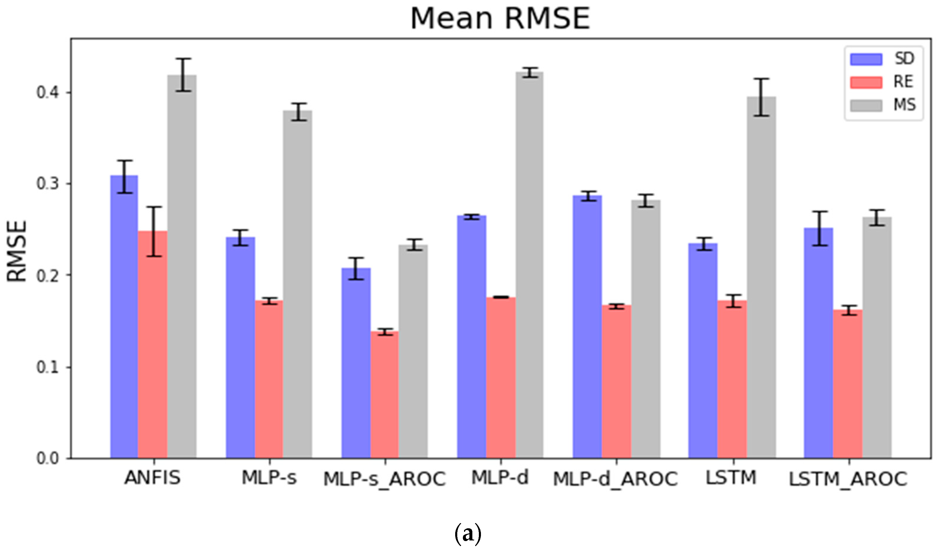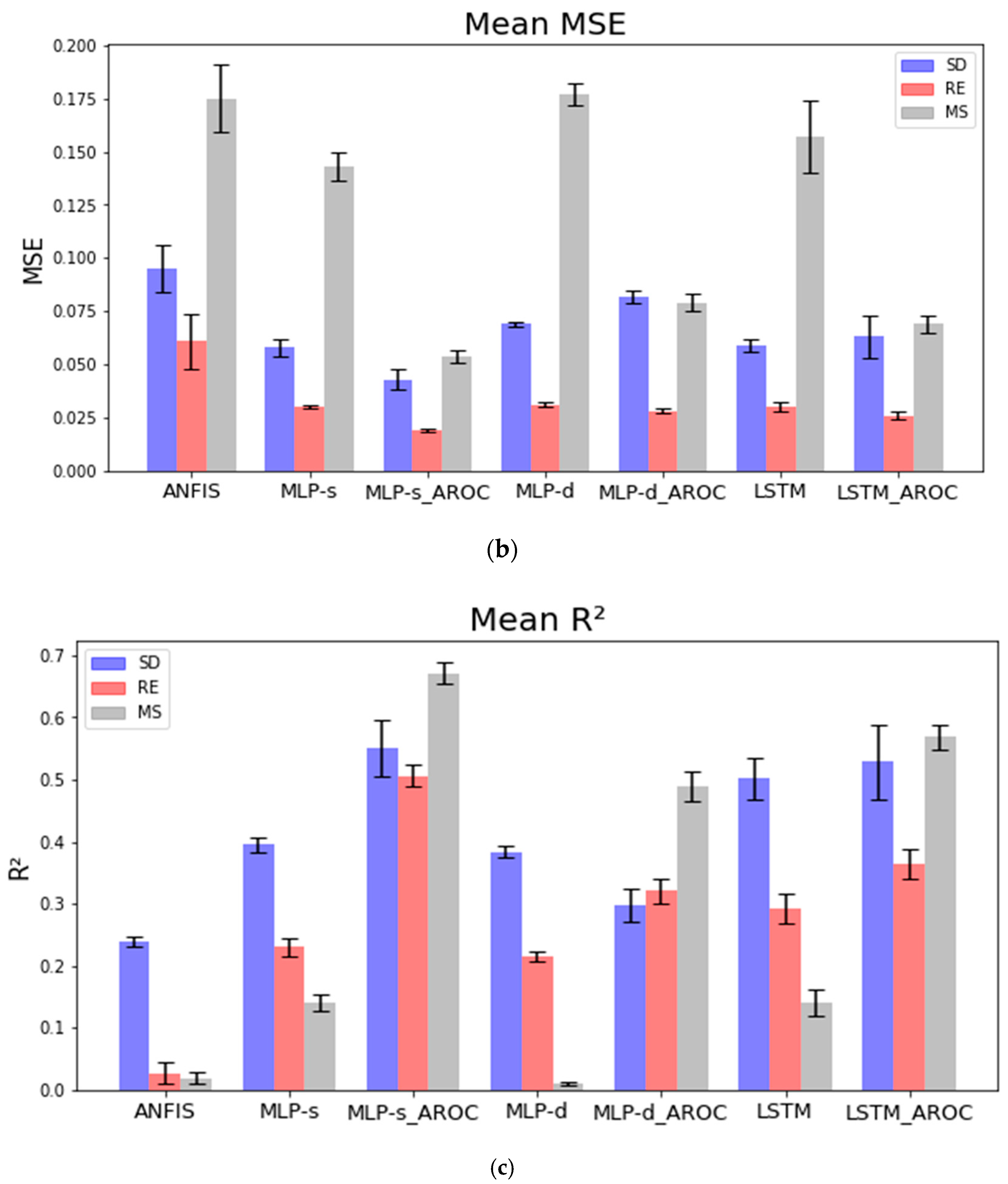The results in Figure 3 show that all models with AROC drastically improved their accuracy, except for LSTM, which only showed a slight increase for subjects RE and MS.

LSTM is well known for its ability to predict time-series-based data sets. This is because the LSTM network has a cell consisting of input gate, output gate, and forget gate. This cell is called an LSTM cell. While the model has an architecture of an artificial RNN model, LSTM has feedback connections, making it able to process an entire sequence of data. Based on the result, we understand that LSTM network works best with fewer input variables because of its ability to process an array of samples consisting of current and past data. This helps the network to memorize features during forward past and provides a safe path for backpropagating error [32]. Furthermore, additional AROC provides the network with the average rate of change between the current EMG signal and past EMG signals. Therefore, additional features were provided for a safer path for backpropagating error. Figure 3a–c shows that LSTM_AROC had only a slight increase in accuracy for subjects RE and MS. RMSE and MSE values for subject SD increased instead. However, the R-squared value increased for all three subjects, meaning better linear correlation between the targeted value and predicted value. Based on the results, additional feature values for the LSTM signal may not have a big impact on increasing estimation accuracy, but a higher linear correlation model can detect dorsiflexion during gait.

Further research is still necessary to improve on these findings. In future research, we would like to carry out experiments using a single sEMG sensor with its AROC as input channel, thereby reducing the number of sensors used to one. We also need to investigate the effects of different activation functions and optimizers on neural network models.

5. Conclusions

In our research, the LSTM network had the highest accuracy in terms of estimating acceleration of the toe motion during gait compared to other models. However, the activation function and optimizer can affect the estimation accuracy, as can be seen by MLP-s having better accuracy than MLP-d. This means that a complicated deep learning network does not always result in higher estimation accuracy depending on the scale of the problem. Furthermore, the addition of average rate of change of EMG signals as input increases the estimation accuracy of the network as more information is provided for training. In conclusion, a time-series network such as the LSTM is suitable for designing a robot AFO control system. Rather than applying deeper hidden layers, which can lead to a time-consuming training process, there is a possibility that high accuracy estimation can be achieved even without using deeper hidden layers. Lastly, feature values such as AROC has the ability to reduce the number of sensors used.