Author Contributions
Conceptualization, C.R. and C.G.-C.; methodology, D.H.P.-O. and L.L.L.-L.; software, D.H.P.-O., C.R., L.L.L.-L., J.M. and C.G.-C.; validation, D.H.P.-O., C.R., L.L.L.-L., J.M. and C.G.-C.; formal analysis, D.H.P.-O. and L.L.L.-L.; investigation, C.R., C.G.-C. and J.M.; resources, C.R. and J.M.; data curation, D.H.P.-O., C.G.-C. and L.L.L.-L.; writing—original draft preparation, C.R. and C.G.-C.; writing—review and editing, D.H.P.-O., C.R., L.L.L.-L., J.M. and C.G.-C.; visualization, C.R.; supervision, C.R. and D.H.P.-O.; project administration, C.R. and J.M.; funding acquisition, C.R. and J.M. All authors have read and agreed to the published version of the manuscript.
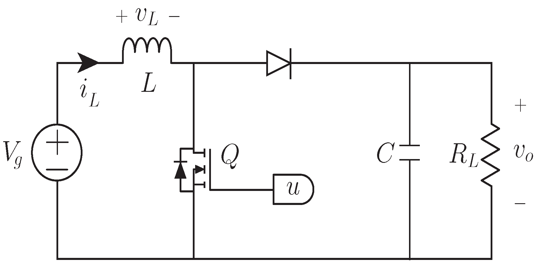
Figure 1.
Schematic of: Boost converter.
Figure 1.
Schematic of: Boost converter.
Figure 2.
BP365 PV module characteristic at (a) C, (b) C, (c) C.
Figure 2.
BP365 PV module characteristic at (a) C, (b) C, (c) C.
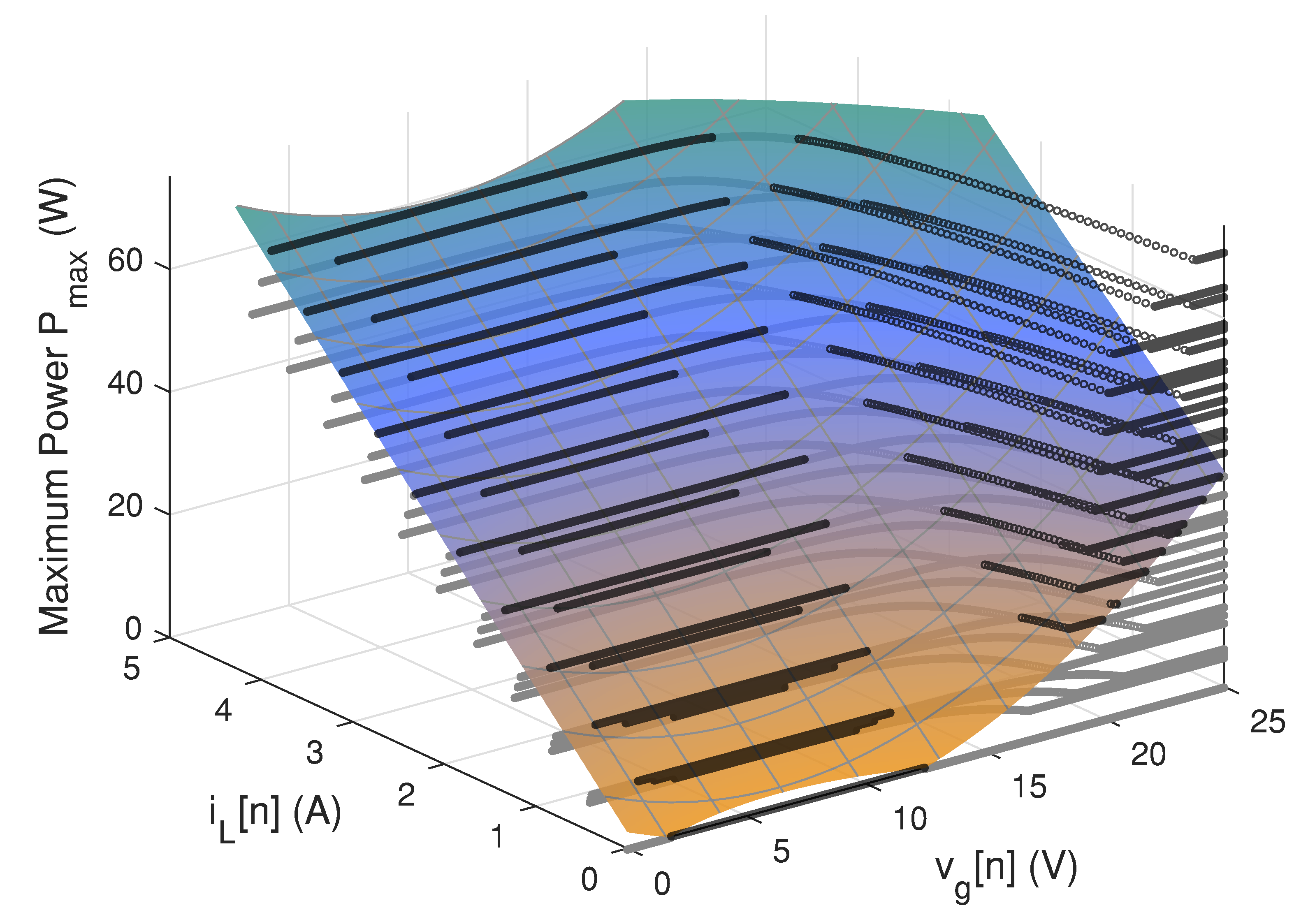
Figure 3.
Plotting of the MPP surface in terms of and .
Figure 3.
Plotting of the MPP surface in terms of and .
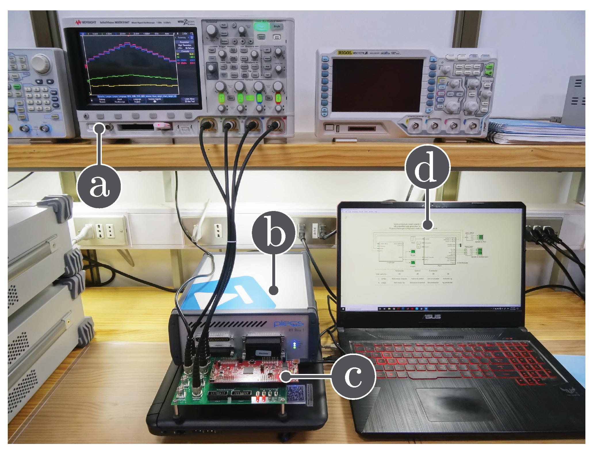
Figure 4.
Hardware in-the-loop experimental setup: (a) oscilloscope, (b) PLECS RT-box, (c) Texas Instruments LAUNCHXL-F28069M, (d) Laptop.
Figure 4.
Hardware in-the-loop experimental setup: (a) oscilloscope, (b) PLECS RT-box, (c) Texas Instruments LAUNCHXL-F28069M, (d) Laptop.
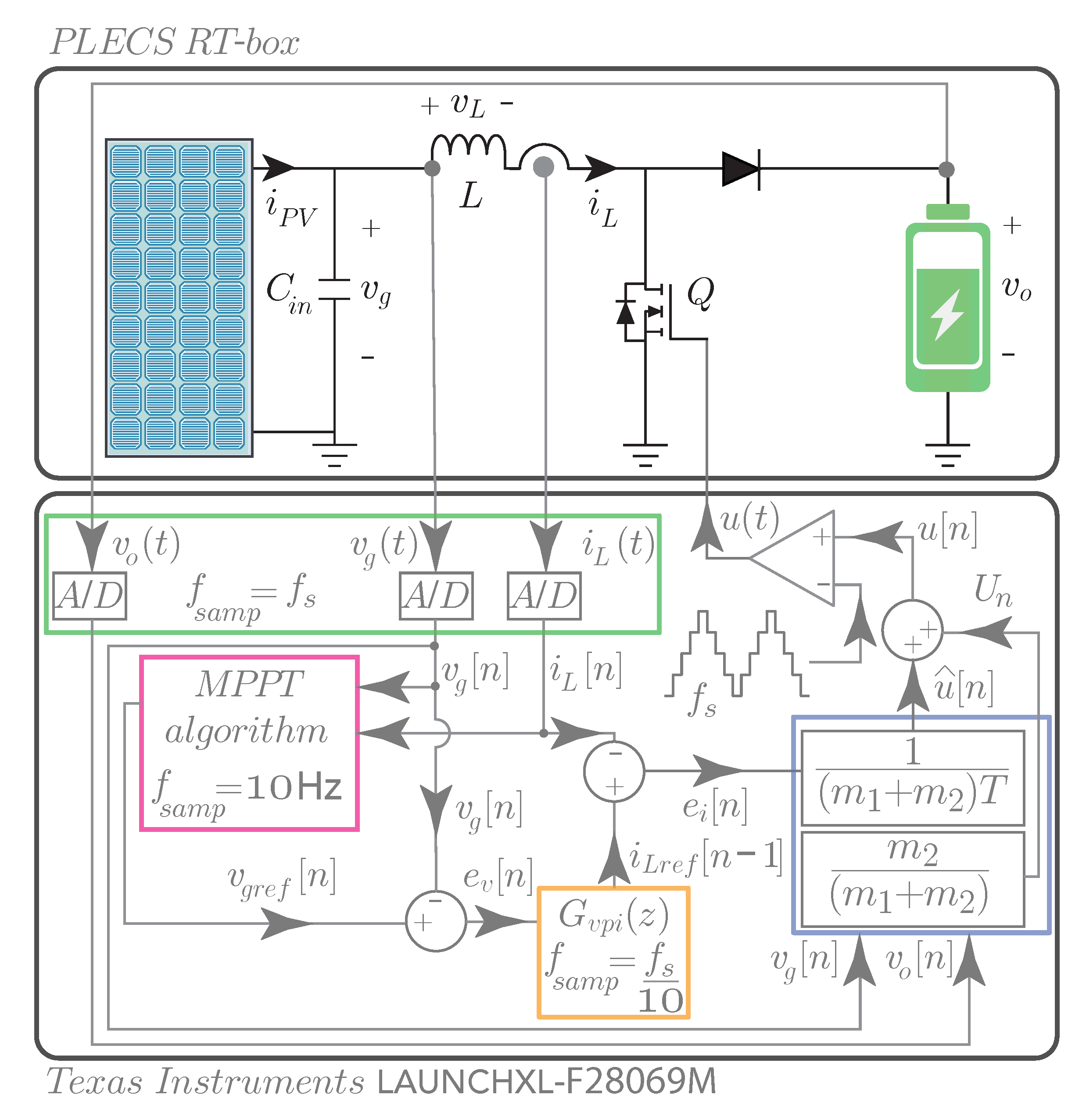
Figure 5.
Block diagram of the digital controller for the MPPT of the boost converter.
Figure 5.
Block diagram of the digital controller for the MPPT of the boost converter.
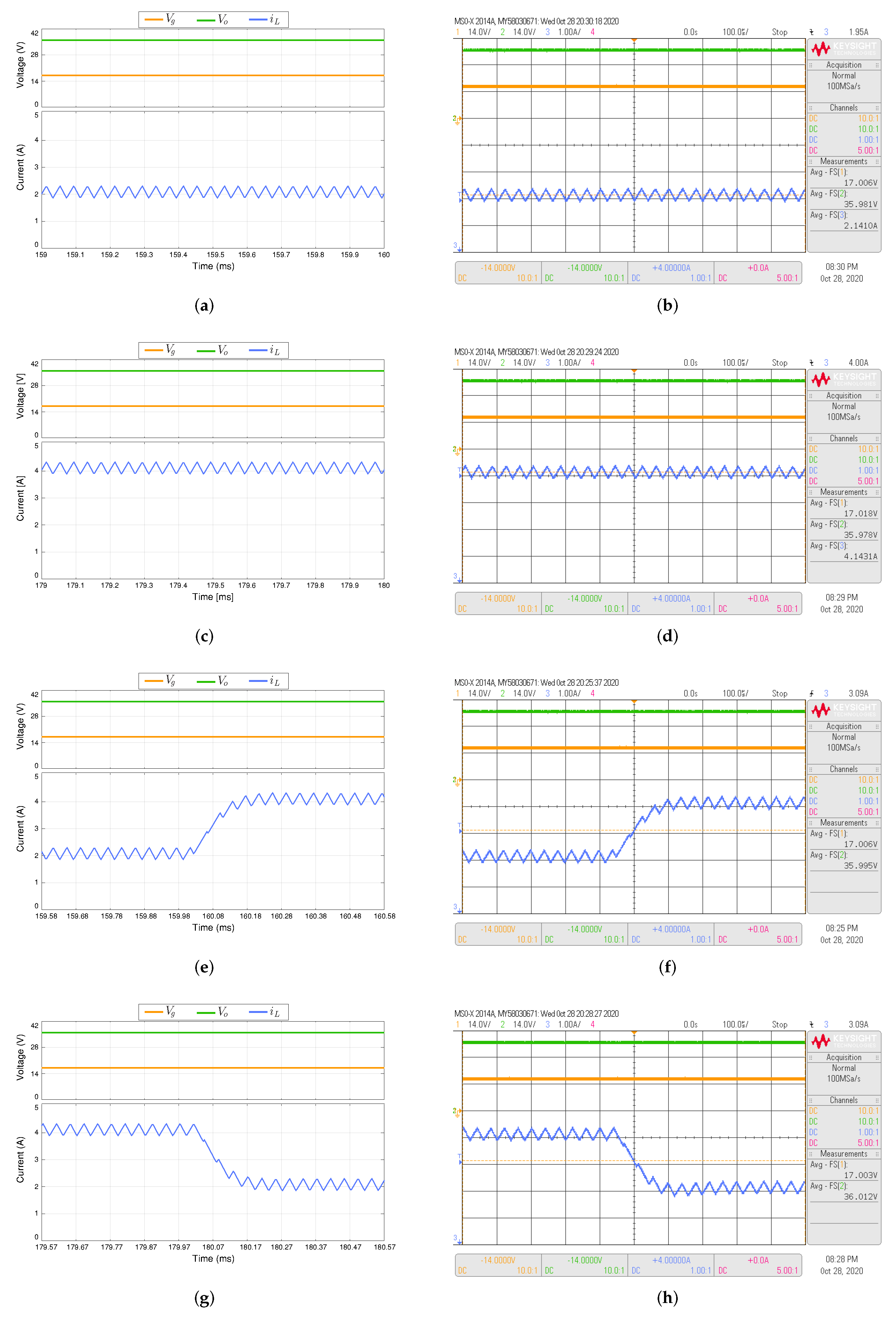
Figure 6.
Simulated (a,c,e,g) and experimental (b,d,f,h) responses of the input current control based on the discrete-time sliding-mode current strategy when the reference : (a,b) is equal to 2 A, (c,d) is equal to 4 A, (e,f) changes from 2 A to 4 A, and (g,h) from 4 A to 2 A. The converter is operating with an input voltage 17 V and an output voltage 36 V). CH1: (14 V/div), CH2: (14 V/div), CH3: (1 A/div) and a time base of 100 s.
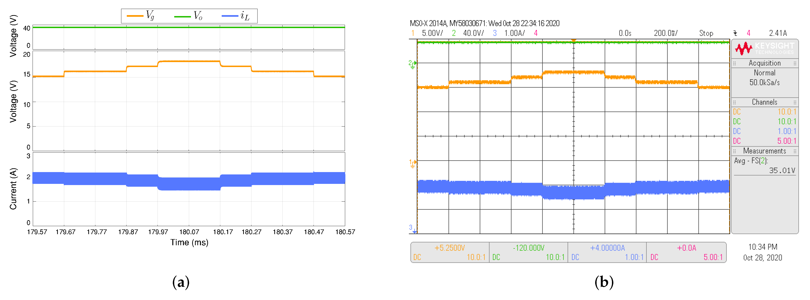
Figure 7.
Simulated (a) and experimental (b) responses of the discrete-time sliding-mode current control when the reference changes with steps of 1 V between 15 V to 18 V while the output voltage ( 36 V) ensures a boost operation. CH1: (5 V/div), CH2: (40 V/div), CH3: (1 A/div) and a time base of 200 ms.
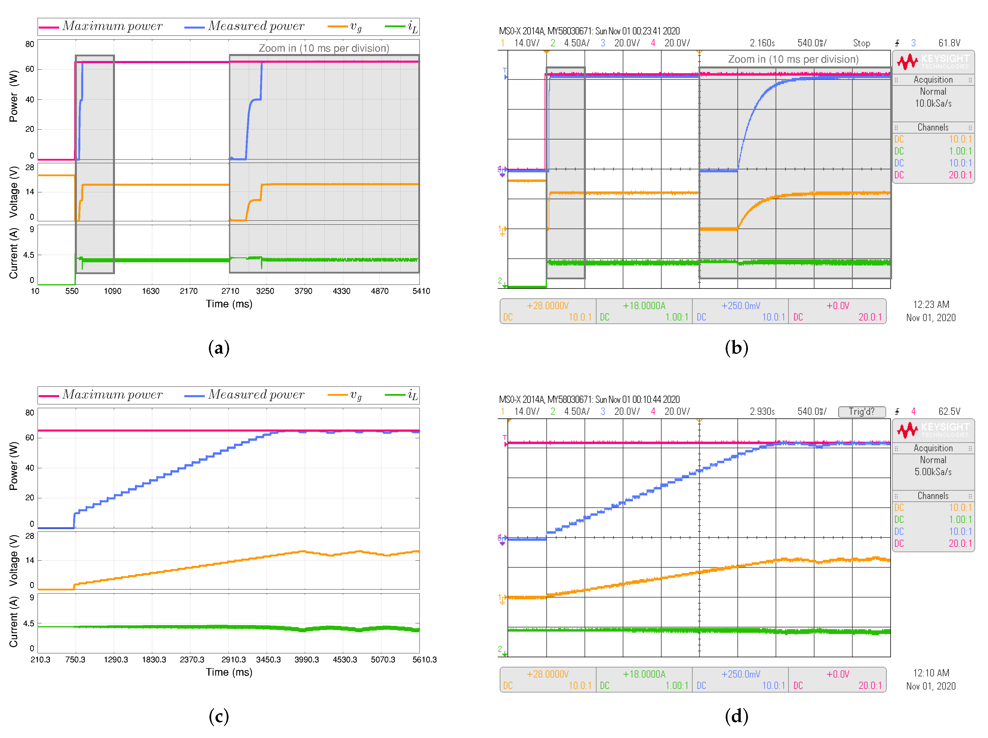
Figure 8.
Simulated (a,c) and experimental (b,d) dynamic behavior of the MPPT algorithms during system start-up with an irradiance of 1000 W/m and an output voltage 36 V. The proposed MPPT algorithm (top) is compared with perturb and observe (P&O)-based MPPT algorithm (bottom). CH1: (14 V/div), CH2: (4.5 A/div), CH3: Maximum power (20 W/div), CH4: Measured power (20 W/div) and a time base of 540 ms and 10 ms in the zoom-in rectangle.
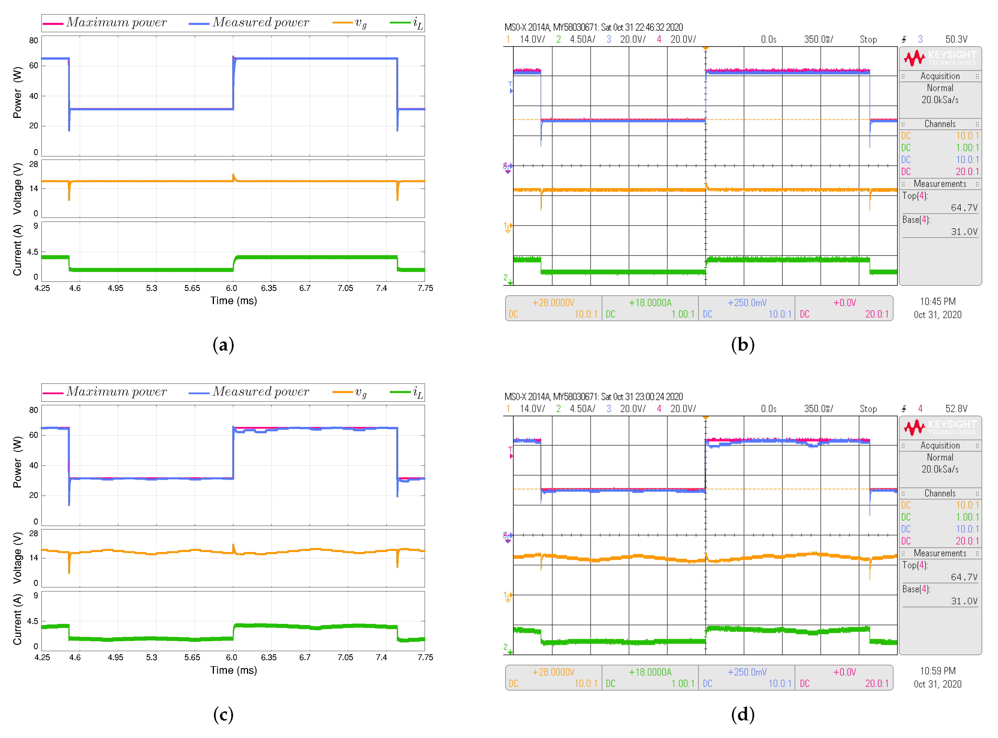
Figure 9.
Simulated (a,c) and experimental (b,d) dynamic behavior of the MPPT algorithms dealing with sudden changes in irradiance between 1000 W/m and 500 W/m and vice versa. output voltage 36 V. The proposed MPPT algorithm (top) is compared with perturb and observe (P&O)-based MPPT algorithm (bottom). CH1: (14 V/div), CH2: (4.5 A/div), CH3: Maximum power (20 W/div), CH4: Measured power (20 W/div) and a time base of 350 ms.
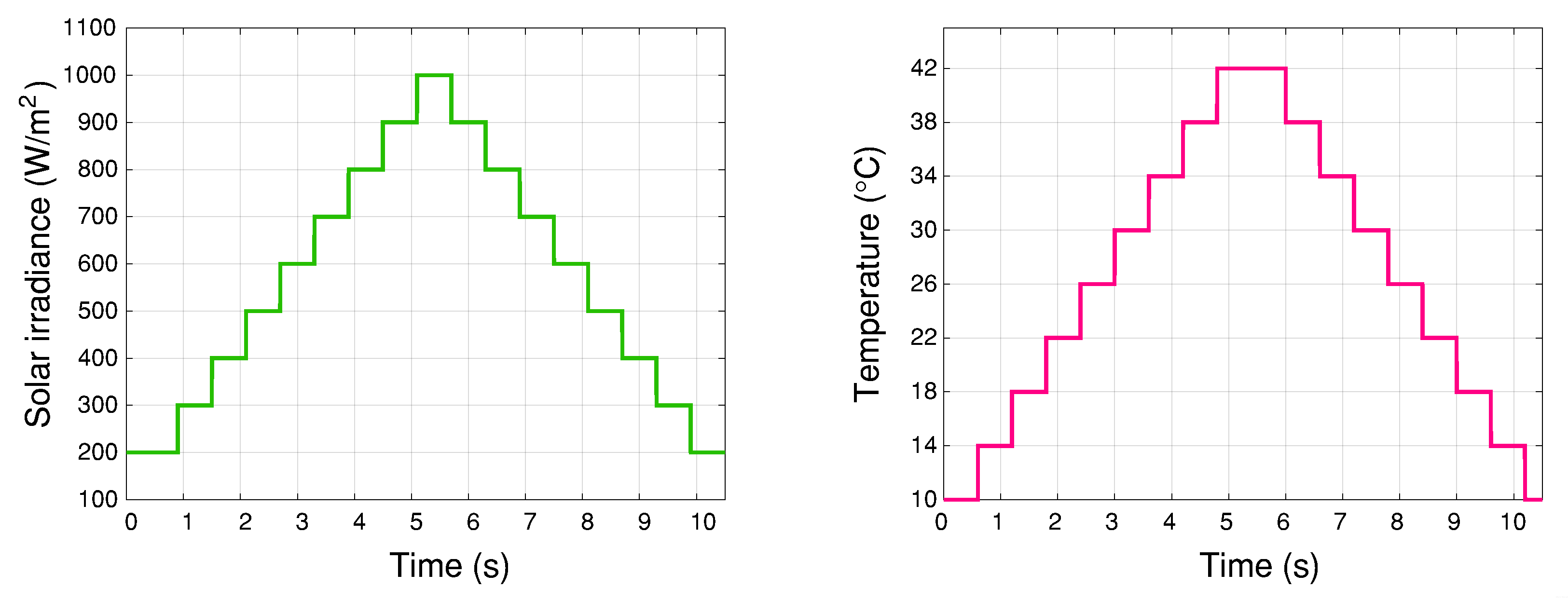
Figure 10.
Irradiance and temperature profile.
Figure 10.
Irradiance and temperature profile.
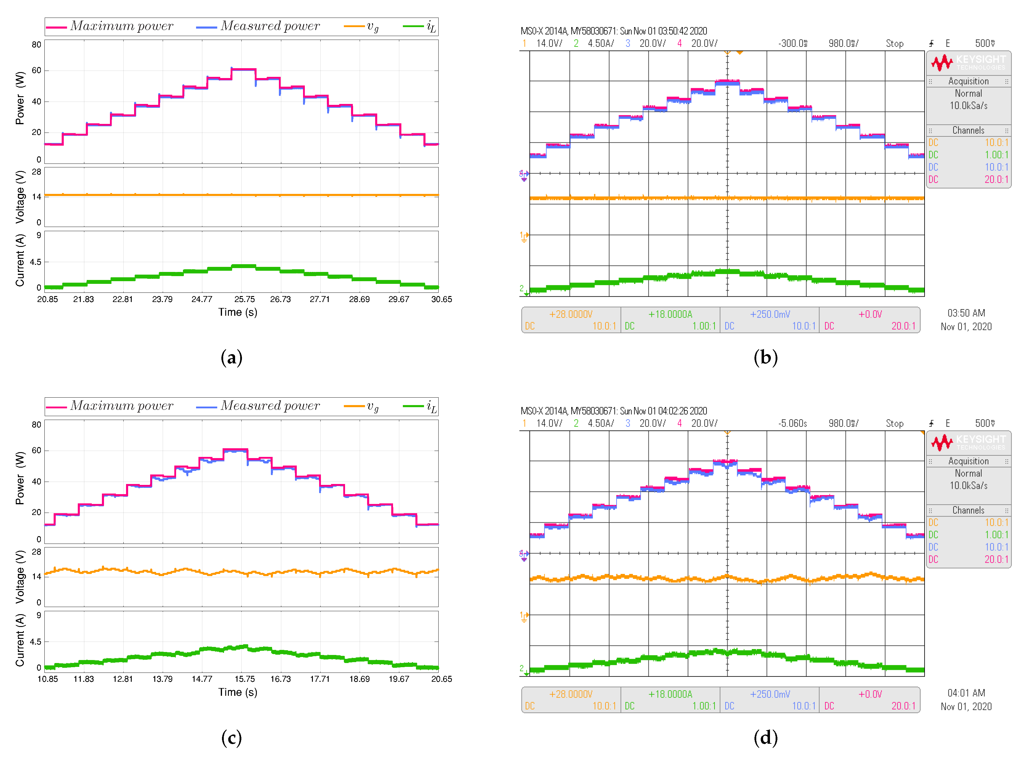
Figure 11.
Simulated (a,c) and experimental (b,d) dynamic behavior of the MPPT algorithms dealing with changes in irradiance and temperature according to the profile shown in (FALTA). Output voltage 36 V. The proposed MPPT algorithm (top) is compared with perturb and observe (P&O)-based MPPT algorithm (bottom). CH1: (14 V/div), CH2: (4.5 A/div), CH3: Maximum power (20 W/div), CH4: Measured power (20 W/div) and a time base of 980 ms.
Table 1.
Slope of the inductor current waveform.
Table 1.
Slope of the inductor current waveform.
| Converter | | |
|---|
| Boost | | |
Table 2.
Examples of polynomial models for surfaces.
Table 2.
Examples of polynomial models for surfaces.
| Polynomial Models | Equations |
|---|
| |
| |
| |
Table 3.
Polynomial model terms.
Table 3.
Polynomial model terms.
| Degree of Term | 0 | 1 | 2 |
|---|
| 0 | 1 | y | |
| 1 | x | | |
| 2 | | | - |
| 3 | | - | - |
Table 4.
Electrical characteristics of Pv module BP 365.
Table 4.
Electrical characteristics of Pv module BP 365.
| Electrical Parameters | Value |
|---|
| Maximum power | 65 W |
| Voltage at maximum power | 17.6 V |
| Current at maximum power | 3.69 A |
| Short-circuit current | 3.99 A |
| Open-circuit voltage | 22.1 V |
| Temperature coefficient of short-circuit current | %/C |
| Temperature coefficient | mV/C |
Table 5.
Comparison of HIL results.
Table 5.
Comparison of HIL results.
| MPPT Algorithm | MPPT-P&O | MPPT-SPF Algorithm |
|---|
| Parameters knowledge | Not necessary | Not necessary |
| Complexity | Low | Low |
| 3680 ms | 18 ms |
| Efficiency | 97% | 99.2% |
| Precision | Low | High |
Table 6.
Comparison of MPPT methods.
Table 6.
Comparison of MPPT methods.
| MPPT Algorithm | P&O | SPF | FESC | SM-ESC | SMPPT |
|---|
| Complexity | Low | Low | Medium | Medium | Medium |
| Efficiency | 97% | 99.2% | 98.34% | 97.51% | 98.95% |
| Precision | Low | High | Medium | Low | Medium |
| Computational cost | Low | Medium | Medium | Medium | Medium |

 ,
, 


