A Three-Stage Data-Driven Approach for Determining Reaction Wheels’ Remaining Useful Life Using Long Short-Term Memory

Abstract

Reaction wheels are widely used in the attitude control system of small satellites. Unfortunately, reaction wheels failure restricts the efficacy of a satellite, and it is one of the many reasons leading to premature abandonment of the satellites. This study observes the measurable system parameter of a faulty reaction wheel induced with incipient fault to estimate the remaining useful life of the reaction wheels. We achieve this goal in three stages, as none of the observable system parameters are directly related to the health of a reaction wheel. In the first stage, we identify the necessary observable system parameter and predict the future of these parameters using sensor acquired data and a long short-term memory recurrent neural network. In the second stage, we estimate the health index parameter using a multivariate long short-term memory network. In the third stage, we predict the remaining useful life of reaction wheels based on historical data of the health index parameter. Normalized root mean squared error is used to evaluate the performance of the various models in each stage. Additionally, three different timespans (short, moderate, and extended in the scale of small satellite orbit times) are simulated and tested for the performance of the proposed methodology regarding the malfunction of reaction wheels. Furthermore, the robustness of the proposed method to missing values, input frequency, and noise is studied. The results show promising performance for the proposed scheme with accuracy in predicting health index parameter around 0.01–0.02 normalized root mean squared error, the accuracy in prediction of RUL of 1–2.5%, and robustness to various uncertainty factors, as discussed above.

1. Introduction

In recent years, small satellites have become our subject of interest due to their low manufacturing cost, ease of launching into orbit and the capability to deliver the same outcome as their large counterparts. Reaction wheels (RW) are an integral part of the attitude control system of a small satellite to have control over the rotation about its axes. To perform the designated task, a satellite needs to have accurate control over its direction. Though RWs are very efficient, they are prone to failure, and for a small satellite, that can lead to a disaster resulting in its complete failure. As there is not much room for mechanical redundancy in a small satellite to enhance the reliability and useful lifetime, one needs to increase the analytical redundancy as an alternative solution. If we properly monitor the performance degradation in the attitude control system components (e.g., RWs) and estimate the system’s remaining useful life (RUL), we can avoid a potential disaster and downtime of the service. Although it may not be financially sound or technically possible to change a defective RW unit on a satellite in orbit to continue its mission; one can argue that the knowledge of the RUL for the actuators onboard a satellite can help plan alternative remedies in case the satellite fails or malfunctions in orbit. The remedial actions can include planning a replacement satellite launch, modifying the mission scope for the malfunctioning satellite, or changing actuators or control schemes onboard the malfunctioning satellite if redundant units are available. The cause of mechanical failure in RWs is often inadequate, bearing lubrication and uneven frictional torque [1]. This fault can be monitored from motor torque constant variation. This study develops a data-driven fault prognosis model to predict the RUL of a faulty RW onboard satellite.

Many studies are found in condition-based monitoring (CBM) and prognostics health monitoring (PHM). However, only a few are dedicated to satellite RWs. Studies show a 200% growth in microsatellites launches in the last five years [2]. It draws attention to develop a data-driven approach that can take the measurable sensor data as input and return the expected RUL of the system under incipient fault. Developing a model-based prognostic method for a complicated system is very difficult as it requires extensive system information. To our knowledge, there are a limited number of studies [3,4,5] found that involve model-based techniques for prognosis. The authors in [1] have proposed a model-based approach to predict the RUL of RWs onboard satellites. The authors claim the model performs considerably well in RUL prediction with the error ranging from 1.5 to 13 percent, but the prediction interval shows the uncertainty in prediction increases with time.

The authors in Ref. [6] have developed a two-step data-driven approach using the Kolmogorov–Smirnov test, self-organize map, and an unscented Kalman filter (UKF). In step one, the authors model the degradation process by learning the degradation. In the second step, degradation data and UKF are combined to predict the RUL. However, the method requires a significant amount of training data to perform meaningfully. In Ref. [7], the authors have developed and implemented a multi-scale extended Kalman filter (EKF) using telemetry data from an RW onboard a satellite to predict its RUL. An ordinary differential equation expresses the motor’s dynamic behavior in the process, and the authors use the damping coefficient as a health indicator. The statistical model-based and data-driven approaches for machine fault diagnosis and prognosis are also discussed in Ref. [8]. In Ref. [9], the authors have used machine learning techniques to automatically detect anomalous spacecraft behavior from telemetry data over a space of seven years. Although telemetry data in Ref. [9] add tremendous value to the work outcomes, the scope of the study is limited to the classification of faults and detection of anomalous behavior rather than RUL prediction.

The authors in Ref. [10] have defined and combined three goodness metrics of correlation, monotonicity, and robustness of the rolling element for degradation feature selection during the RUL prediction. In Ref. [11], the authors have used wavelet packet transform (WPT) and an artificial neural network (ANN) for rolling element RUL prediction. Both proposed methods can be used for any similar system, and the outcome and robustness can be improved if the model can be trained with data from multiple systems. In [12], the authors have used experimental data and suggested a condition monitoring technique for bearing life enhancement and preventing torque inequality by controlling the lubrication process.

The authors propose a method using support vector machine (SVM) regression in Ref. [13] for wear assessment of cutting tools and calculation of RUL. The proposed method is based on feature extraction, and it requires adequate training data for the model to predict meaningfully. The method uses a combined feature found by dimensionality reduction and uses it as a health index (HI) parameter. Ultimately, the HI parameter is mapped to a nonlinear regressor for RUL prediction. In Ref. [14], variational mode decomposition (VMD) and long short-term memory (LSTM) recurrent neural networks (RNN) are used for the prediction of rotary machinery health. The authors in Ref. [15] have used a feed-forward ANN with a Marquardt training algorithm to predict the RUL of a bearing. The proposed ANN model uses time and measurements of Weibull Hazard rates of root mean squared (RMS) and kurtosis from its present and previous points as input and returns normalized life percentage as output.

The authors in Refs. [16,17,18,19,20] have studied and implemented different available techniques for the prognosis of rotary machinery. Different stages of CBM and PHM are mentioned in these articles, such as data collection, feature selection, and state prediction using ANN. The authors have summarized several contemporary works in prognosis up to the date of publication of their research.

In Ref. [21], the authors mentioned an intelligent technique for the CBM and PHM of the common rotary component in a system. In this process, vibrational data from the sensor is used as an input, and feature extraction is carried out using a sparse auto-encoder. The authors used a moving average filter before feeding the data to the model, which returns an auto-encoder correlation-based rate (AEC) as output, and AEC is used to understand the condition of the rotary machinery. A method for CBM of rotary machinery using vibration data and the sound of working conditions is also mentioned in Ref. [22].

In Ref. [23], the authors used the Fourier transform and an auto-encoder to identify high-level features for PHM of rotary machinery. The model predicts the RUL with reasonably good accuracy, but the model performance degrades with noise. The model can be used in a similar scenario of PHM in any system where vibration analysis is used. In Ref. [24], the authors have studied acoustic emission, vibration data, acoustic technique, the shock pulse method, thermal and wear debris monitoring for CBM of mechanical and electrical devices.

The authors in Ref. [25] have proposed a multidimensional technique using SVM and particle filter-based method for PHM of rotary machinery; the approach in their study is claimed to be better in estimating RUL than the methods using data from single sensors. On the contrary, the model complexity in Ref [25] is higher, making it unsuiTable for complex systems that require a faster response.

Some statistical model-based and data-driven approaches for CBM and PHM are briefly discussed in Ref. [8]. The authors in Refs. [26,27,28] have used the COVID-19 data set of infected people to predict the peak during the wave of infection and estimated time to reach that state, while the authors have used different state-of-the-art machine learning techniques for the regression analysis in these papers.

LSTM is an effective RNN for regression analysis and feature selection. The fundamentals and different applications of the LSTM model are discussed in Refs. [14,29,30,31,32]. The authors of Ref. [33] have proposed a two-step prognosis technique for satellite RWs and carried out a state parameter prediction. The authors used an auto-regressive integrated moving average (ARIMA) model and an LSTM network for state parameter prediction, and the best accuracy obtained by each model has a normalized root mean squared error (NRMS) of 0.138 and 0.04, respectively.

The majority of the published literature focuses on single- or two-step approaches to tackle the problem of remaining useful life prediction for reaction wheels with moderate performance evaluated based on NRMS. The proposed methods in the literature are either too complex, with high computation costs, or have inferior performance if the model complexity is not significant. There is a gap for a methodology that is neither too complex with high computational costs nor performs inferior to the existing complex and computationally expensive methods.

This study proposes a three-step data-driven approach for the prognosis of reaction wheels using LSTM. In the first step, we carry out state prediction. In the second step, we define and predict the health index parameter (parameter prediction). Finally, in the third step, with the help of historical data and a threshold, we predict the RUL of RW ITHACO Type-A by Goodrich as a case study. The novelty of this work is in developing a new three-stage data-driven prognostic technique using LSTM, which is not complex with high computational costs and performs reasonably with accuracies achieved in the prediction of HI around 0.01–0.02 NRMS error, and the accuracy in prediction of RUL of 1–2.5%.

The remaining of this paper consists of the following sections: in Section 2, we describe the problem in satellite RW fault prognosis, while The detailed methodology to solve this problem is discussed in Section 3. Next, in Section 4, we implement the proposed methodology for the evaluation of the model. Finally, in Section 5, we conclude with the usefulness of the proposed model in a real-life application and the future scopes of research.

2. Problem Statement

Reaction wheels were first introduced in automobiles to conserve momentum and provide smooth power output, and the same idea can be used for many purposes. In a satellite attitude control system, the reaction wheels are used for a different purpose. Particularly in small satellites, RWs are used to rotate the satellite on its axes. This is achieved by using an electric motor to rotate the RW to obtain an equal and opposite momentum to rotate the satellite in the opposite direction, and multiple RWs can be assembled in different configurations to gain 3-axis attitude control. As a result, the method has become very popular for cost-efficient satellite manufacturing and servicing. However, the reaction wheel as a mechanical device does not have a long lifespan, and in the case of small satellites, there is not much room for mechanical redundancy to improve reliability.

Furthermore, installing an increased number of RWs in satellites increases the weight and launch costs, which contradicts the key financial aspect of small satellites. To overcome this problem, proper CBM and PHM techniques can be used to increase service reliability as it will nullify the service downtime due to RW failure by providing an estimated RUL of the system. As mentioned earlier, although this may not be financially sound or technically possible to change a defective RW unit on a satellite in orbit to continue its mission, one can argue that the knowledge of the RUL for the actuators onboard a satellite can help plan alternative remedies in case the satellite fails or malfunctions in orbit. The remedial actions can include planning a replacement satellite launch, modifying the mission scope for the malfunctioning satellite, or changing actuators or control schemes onboard the malfunctioning satellite if redundant units are available.

This study aims to predict the remaining useful life of a reaction wheel under incipient fault using a data-driven approach. To achieve this goal, a three-step process is proposed. Figure 1 illustrates the flow of the proposed three-step process followed during the prognosis of RW in this study. In the first step, we carry out a state parameter prediction, where unseen system states are predicted based on current and historical system states. In the second step, we define and predict the health index parameter, where the degradation model is generated based on the data from measurable states (wheel speed ${\omega }_m$ and motor current $I_m$) to determine the values of unmeasurable or unavailable system parameters (motor torque constant $k_t$ and bus voltage $V_{bus}$) that can be represtative of faults or anomalies in RW behavior. Finally, in the third step, the $k_t$ predicitions are used to intersect with the RW failure threshold of (30% nominal) to determine the RUL of the RW.

The main components of RW that are prone to failure are bearing and electrical motor. The developing fault can be monitored by motor torque constant ($k_t$) and bus voltage ($V_{bus})$, neither of which can be directly measured from the sensor readings. The available essential sensor readings are wheel speed (${\omega }_m$), motor current ($I_m$), and voltage input ($V_{comm}$) as shown in Figure 2.

The mathematical relation between system states motor current $I_m$, RW speed ${\omega }_m$ and HI parameter motor torque constant ($k_t$) is expressed in Equation (1), and it can be seen that the relationship between these states and parameters is nonlinear [34].

$$\begin{array}{l}{\dot{I}}_m=G_d{\omega }_d\left[f_3\left({\omega }_m,I_m\right)-f_5\left({\omega }_m\right)\right]-{\omega }_d{I}_m+G_d{\omega }_d{V}_{Comm}\\ {\dot{\omega }}_m=\frac{1}{J_w}\left\{f_1\left({\omega }_m\right)+k_t{I}_m\left[f_2\left({\omega }_m\right)+1\right]-{\tau }_v{\omega }_m-{\tau }_c{f}_4\left({\omega }_m\right)+{\tau }_{noise}\right\}\end{array}$$

(1)

There are five building blocks ($f_{1-5}$) inside Bialke’s RW model, which are discretized by Sobhani-Tehrani in Equation (1) [34] and Figure 2. In Figure 2, $f_1$ and $f_2$ capture the motor disturbance, $f_3$ accounts for EMF torque-limiting block, $f_4$ addresses the analytical approximation of the sign function, and $f_5$ stands for the speed limiter block. A detailed explanation of these blocks and Equation (1) can be found in Ref. [34].

Figure 2 represents Bialki’s ITHACO type-A reaction wheel by Goodrich. The system parameters and constants for this reaction wheel are listed in

Table 1. ITHACO Type-A reaction wheel model parameters.

Parameter	Value
Coulomb Friction (${\tau }_c$)	0.002 Nm
Viscous Friction (${\tau }_v$)	3.84×10−4 Nm/rad/s
Drive gain time constant (${\tau }_d$)	0.245
Ripple Torque (B)	0.22
Temperature ($T$)	23 °C
Cogging Torque (C)	0
Torque Noise Frequency (${\omega }_a$)	0.2 rad/s
Jitter Angle (${\theta }_a$)	0.05 rad = 3 degrees
BEMF ($k_e$) Nominal	0.029 V/rad/s
Motor Torque Const. ($k_t$)	0.029 Nm/A
Bus Voltage ($V_{bus}$) Nominal	8 V
Bridge Resistance ($R_B)$	2 $\mathsf{\Omega }$
Driver Gain ($G_d$)	0.19 A/V
Number of Motor Poles (N)	36
Input Filter Resistance ($R_{IN}$)	2 Ω
Quiescent Bus Power ($P_q$)	3 W
Driver Bandwidth (${\omega }_d$)	9 rad/s
Voltage Feedback Gain ($k_f$)	0.5 V/V
Over-speed Circuit Gain ($k_s$)	95
Maximum Wheel Speed (${\omega }_s$)	680 rad/s

. Due to the nonlinearity in the mathematical relation, numerical simulations are used to generate accurate input data. A detailed description of Bialke’s high fidelity reaction wheel model can be found in [35]. As mentioned earlier, our study used Sobhani-Tehrani’s [34] adaptation of Bialke’s model to implement numerical simulations and generate assimilated data for our study, as discussed in the following sections.

Figure 2. Bialke’s ITHACO Type-A reaction wheel model [35].

Figure 2. Bialke’s ITHACO Type-A reaction wheel model [35].

Our research aims to develop a data-driven model for the prognosis of RWs in a three-step process. Although the methodology should be applicable to other systems, the reaction wheel system is used for the proof of concept. The relation between the states and the HI parameter is highly nonlinear in [34]. Therefore, in the first stage of our work, we forecast the future data (RW speed (${\omega }_{t+1}$), motor current ($I_{m_{t+1}}$), torque command voltage ($V_{com{m}_{t+1}}$) using a forecasting model and the available measurements (RW speed (${\omega }_t$), motor current ($I_{m_t}$), torque command voltage ($V_{Com{m}_t}$) ). In the second stage of the proposed approach, we define the HI parameters to be $k_t$, and employ a degradation model to find forecasted states for these parameters using the degradation model and historical and available measurements from the system. Finally, in the third stage of the proposed approach, we establish a threshold for the HI parameter ($k_t$) from the HI data and compare with the data found in the second stage to predict the RUL.

3. Methodology

There are three major categories of prognostic works in the field. These methods include model-based, semi-model-based, and data-driven. Model-based techniques are very accurate and popular for less complicated systems as they require a lot of system information. It is challenging to build a comprehensive model-based prognostic technique for a complicated system. This is where semi-model-based and data-driven techniques shine. The main advantage of using data-driven techniques is that they do not require much system information, rely more on the inputs and outputs available from measurements, and can be equally effective for any similar system. Our study found the LSTM network very efficient in predicting future states from the available measurements.

Figure 1 shows the flow of the three main steps towards building our prognostics model for a RW. As briefly discussed, in the first step, we carry out state parameter prediction where unseen system states are predicted based on current and historical system states. In the second step, we define and predict the health index parameter, where the degradation model is generated based on the data from measurable states (wheel speed ${\omega }_m$ and motor current $I_m$) to determine the values of unmeasurable or unavailable system parameters (motor torque constant $k_t$ and bus voltage $V_{bus}$) that can be representative of faults or anomalies in the RW behavior. Finally, in the third step, the $k_t$ predictions are used to intersect with the RW failure threshold of (~30% nominal) to determine the RUL of the RW. In the following sub-sections, additional details on each step of the three-step process are provided, followed by results and discussions in the next section.

3.1. Data Collection and Preparation

Generally, for data-driven prognosis approaches, the raw data to train and test a model are collected from the functioning hardware or a computer simulation from a digital twin of the hardware. The real-life data from a satellite attitude control system not easily accessible, making the data-driven fault prognosis more difficult. We overcome this by producing synthetic data from a computer-generated model. We use Bialke’s ITHACO Type-A high fidelity model, as shown in Figure 2 and formulated in Equation (1), to generate synthetic data and add Gaussian white noise to the dataset to resemble the dataset from a real-life unit.

For the simulation, we set all the RW parameters as listed in Table 1, and we inject an incipient fault in the $k_t$ parameter of the model as

$$k_t=k_t{}_0\left(\frac{1}{e^{t\times {10}^{-4}}}\right)$$

(2)

where $k_t{}_0$ is the initial or nominal value for $k_t$ and $t$ is the time in the simulation. As can be seen, Equation (2) is an exponential decline from the $k_t{}_0$ value, which can be a common representation of incipient degradation or fault in system parameters. In our simulations, $k_{t_0}=0.029$ from Table 1.

We run the model for and store the model output at every 0.1 seconds during the simulation into the comma separate value (CSV) file. The model outputs are RW speed (${\omega }_m$), motor current ($I_m$), Torque command voltage ($V_{comm}$), motor torque constant ($k_t$), and bus voltage ($V_{bus}$), where ${\omega }_m$, $I_m$, and $V_{comm}$ are the measurements that are available from sensor reading and $k_t$ and $V_{bus}$ are non-measurable system parameters that we can use for RW health monitoring. All CSV-stored data are used for analyzing and building a data-driven fault prognosis model in the following steps. We then add Gaussian white noise to the dataset to resemble the dataset from a real-life satellite.

Missing Data Imputation and Noise Addition

In our study, we use model-generated data, making our dataset free from impurity. However, there can be missing values, additional disturbance, or noise in real-life datasets due to errors in the sensor reading or other uncertainties. To ensure real-life implication, it is crucial to address these issues. We randomly erased data from the simulated dataset to emulate missing data or sensor reading issues. When working with missing data, interpolation techniques are used to impute the missing values. In Equation (3), the interpolation function for missing value imputation can be found.

$$y=y_1+\left(x-x_1\right)\frac{\left(y_2-y_1\right)}{\left(x_2-x_1\right)}$$

(3)

where $x$ and $y$ are the unknown data points and $\left(x_1,y_1\right)$ and $\left(x_2,y_2\right)$ are the known sets to use for interpolation.

We additionally added Gaussian white noise to the dataset to emulate the real-world uncertainties. Equation (4) defines a white Gaussian

$$S_X\left(f\right)=\frac{N_0}{2}, \mathrm{for} \mathrm{all} f,\hspace{1em}\hspace{1em}{\mu }_X=0$$

(4)

where $S_X\left(f\right)$ is the flat power spectral density, ${\mu }_X$ is the mean, and ${\mathrm{N}}_0/2$ is a constant. We calculate and express the noise quantity signal-to-noise ratio (SNR) in decibel in this study. The function used for the calculation of noise level can be found in Equation (5)

$$\mathrm{SNR}=20\log \frac{S}{N}$$

(5)

3.2. LSTM Model

LSTM is a specially designed RNN that can address long term dependency issue that exists with conventional RNNs. LSTM was first proposed by Hochreiter and Schmidhube [29]. Currently, there are many versions of the LSTM network available. However, the LSTM network used in this study is adapted from [36,37,38]. LSTM has a chain-like structure similar to all other standard RNNs; however, the repeating module in LSTM has a different structure with interactive layers. The components of each block inside an LSTM network are shown in Figure 3.

Each block in Figure 3 takes a sequence of input, and a sigmoid function determines the activation of gates inside the block. Equation (6) represents a sigmoid activation function.

$$\sigma \left(t\right)=\frac{1}{1+e^{-t}}$$

(6)

The first step inside an LSTM network block is a forget gate to decide which information to dispose of from the cell state. Equation (7) mathematically represents a forget gate.

$$f_t=\sigma \left(W_f\cdot \left[h_{t-1},x_t\right]+b_f\right)$$

(7)

The next step has two parts. The input gate layer decides which values will be updated in the first part, as shown in Equation (8).

$$i_t=\sigma \left(W_i\cdot \left[h_{t-1},x_t\right]+b_i\right)$$

(8)

In the second part, a $\tanh \left(·\right)$ layer creates new values to add to the state in Equation (9).

$${\tilde{C}}_t=tanh\left(W_C\cdot \left[h_{t-1},x_t\right]+b_C\right)$$

(9)

Later, these two parts are multiplied to update the state in Equation (10).

$$C_t=f_t\times C_{t-1}+i_t\times {\tilde{C}}_t$$

(10)

Finally, the block decides the output in the output gate step. In this step, a sigmoid function first decides which part of the cell state to pass as output, using Equation (11).

$$o_t=\sigma \left(W_o\left[h_{t-1},x_t\right]+b_o\right)$$

(11)

Subsequently, the cell state from the input gate passes through a $\tanh \left(·\right)$ and is multiplied by the output of the output gate, using Equation (12).

$$h_t=o_t\times \tanh \left(C_t\right)$$

(12)

As a result, the output gate inside the LSTM block can provide the final output for the block. In Equations (7)–(12), $W_f$, $W_i$, $W_C$, and $W_o$ are the weights of the forget gate, input gate, $\tanh \left(·\right)$, and output gate, respectively, $h_{t-1}$ is the output from the previous block, $x_t$ is current time steps contribution, $C_{t-1}$ is the contribution of $\tanh \left(·\right)$ from the previous block at time ($t-1$), and terms $b_f$, $b_i$, $b_C$, and $b_o$ are the biases.

3.3. State Prediction (Stage 1)

For our study, available measurements are the RW angular speed (${\omega }_m$), Motor current ($I_m$), and Input voltage ($V_{comm}$). An LSTM network is used for the prediction of future measurements, also known as state reconstruction. The utilized LSTM network incorporates a visible input layer, a hidden layer comprising four LSTM blocks, and an output layer. A customized Adam optimizer is used for learning rate and faster convergence. The Adam optimizer is customized using a scheduler with a learning rate decay rate of 0.85 for every 10 epochs. A large initial learning rate helps the network learn faster and reduce computational time, but it can result in a suboptimal solution [40]. Hence, the use of a scheduler solves the problem for the network to learn faster and efficiently. The model is trained with 70 percent of the dataset and tested with the remaining of the dataset. For validation, 25 percent of the dataset is used. The predicted measurements are stored and used for state or HI parameter prediction. However, when predicting the data after the available dataset, we need to predict based on the prediction in the previous time step. This causes even a minor error in the prediction of the first-time step to propagate through the next prediction. We assist our model in overcoming this problem by using a reference line for the states. The reference line is formed as

$$\begin{array}{ll}{\omega }_m\left(t\right)& =A_1\times e^{\left(\log \left(b_1\right)\times t\right)}\\ & \hspace{1em}\hspace{1em}\hspace{1em}\hspace{1em}+(A_2\times e^{\left(\log \left(b_2\right)\times t\right)})\times sin\left(f_{max}\times \mathsf{\omega }\times t+p\right)\\ & \hspace{1em}\hspace{1em}\hspace{1em}\hspace{1em}+c\end{array}$$

(13)

where, $A_1$, $b_1$, $A_2$, $b_2$, $\omega$, $p$, $c$ are unknown constants, $t$ denotes time, and $f_{max}$ is maximum frequency obtained from a fast Fourier transform (FFT) from the dataset. All unknown constants excluding $f_{max}$ in Equation (13) are found using a nonlinear least-squares fit of the dataset to Equation (13). For $f_{max}$ an FFT is applied to the required state that needs reconstruction (in this case ${\omega }_m$) dataset to find the maximum frequency in the dataset, as shown in Figure 4. The FFT in Figure 4 is the result of ${\omega }_m$ data generated from the simulator and passed through an FFT to identify dominant frequencies in the data and choose the highest frequency in the FFT as the value for the $f_{max}$ in Equation (13). Once $f_{max}$ is identified from the ${\omega }_m$ dataset and substituted in Equation (13), a nonlinear least-squares fit is used to find the remaining unknown constants in Equation (13) and obtain the final tren line for ${\omega }_m$.

Using the obtained $f_{max}$ from Figure 4 as $0.003201$ in Equation (13) and using a nonlinear least-squares fitting approach with the ${\omega }_m$ dataset shown in Figure 5 as input, as well as Equation (13) with a substituted value of $f_{max}$ as output form will result in $A_1=8.617$, $b_1=5.601$, $A_2=0.999$, $b_2=0.999$, $\omega =6.249$, $p=0.304$, $c=0.441$. The comparison between the fitted curve and the original data is shown in Figure 6.

The results from Figure 6 show a good match between the original dataset and the fitted model using a combination of FFT and nonlinear least-squares regression. As mentioned earlier, since slightest mispredictions in future system states (${\omega }_m$ and $I_m$) can result in major deviations in HI parameter ($k_t$ or $V_{bus}$) predicitions. Therefore, using a fitted model for future state reconstruction that can be used by the predictor to estimate HI values based on system states, deemed necessary in the successful formulation of the methodology for this study.

3.4. HI Parameter Prediction (Stage 2)

The main goal of our study is to predict the remaining useful life of the reaction wheel, so we determine the HI parameter ($k_t$) in this stage from measurable sensor data, that is, the angular wheel speed (${\omega }_m$) and motor current ($I_m$). A multivariate LSTM network is used for the calculation of HI parameter motor torque constant ($k_t$). We take wheel speed (${\omega }_m$), motor current ($I_m$), and torque command voltage ($V_{comm}$) as inputs to train the model, and we calculate loss during training from the available motor torque constant data from the model. A total of 70 percent of the total data is used during training, and the rest are used to test the model performance. For validation, 30 percent of the dataset is used. A custom Adam optimizer with a decremental learning rate is used for efficient training.

As there are different types of frequencies in the input data, we use three filters in the input data before feeding them to the model to assist model performance. For RW speed data, we use an exponential trend filter as,

$$y\left(t\right)=a\times \left(e^{-\left(b\times t\right)}\right)+c$$

(14)

where the unknown constants $a, b, c$ are found using a nonlinear least-squares fit for motor current and torque command voltage data. The values of unknown constants in the equation are found using the curve_fit function from Python library SciPy. Initially, all the constant values are set to 1 and using nonlinear least square optimization, the curve_fit function estimates the values of the unknown constants fitting an exponential to the dataset. We use a moving average (MA) filter as,

$$\mathrm{Moving} \mathrm{Average} \left(\mathrm{MA}\right)=\frac{A_1+A_2+\cdots +A_n}{n}$$

(15)

where $n$ is the window size for calculation of moving average and $A_i$s are the points in the window that the average is being calculated from.

3.5. Calculation of RUL (Stage 3)

We calculate the remaining useful life based on the predicted value of HI parameter ($k_t$) and a threshold value for it. As stated in [41], the threshold is based on the nominal value of motor torque constant ($k_t$). If the degraded value of $k_t$ reaches 30 percent of its nominal state value, as listed in Table 1, the system is assumed to have failed. Thus, the intersection between the degradation trend of HI parameter ($k_t$) and its 30% threshold determines the point of predicted failure occurrence. We can calculate the time window from the present to the point of predicted failure to find out the RUL of the RW with incipient fault.

4. Results and Discussion

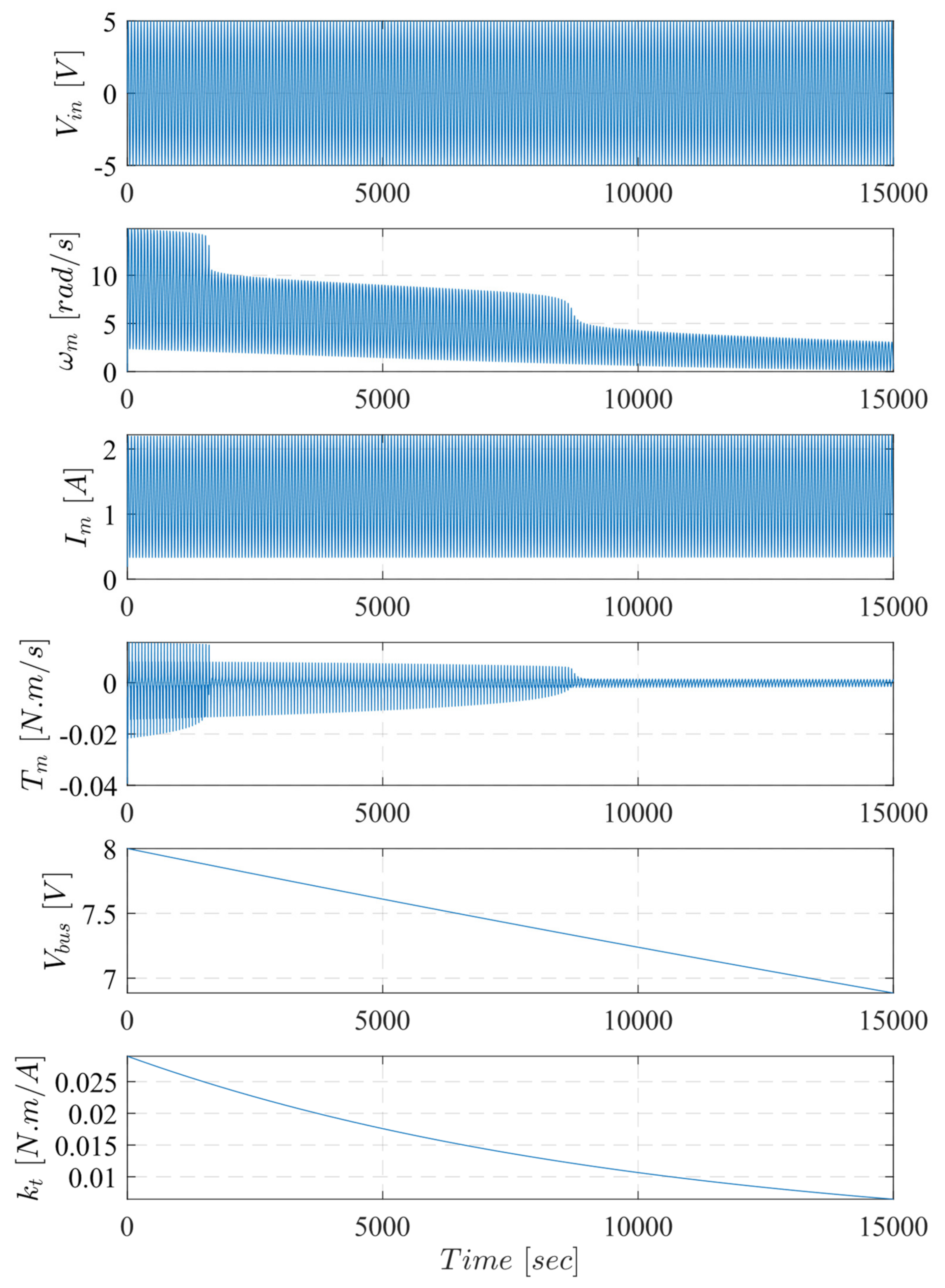
We generate the dataset using a computer simulation in MATLAB, and the simulation is carried out on a Dell computer with an Intel® Core™ i7-4790 CPU with a processing power of 8GHz, Intel® HD Graphics 4600, and 8 GB of RAM. An LSTM network from Python library Keras is used for forecasting future system measurement data, and for state parameter prediction, a multivariate LSTM network is employed. The LSTM network employed for forecasting system measurement is known as vanilla LSTM. This network has an input layer, a visible layer, a hidden layer with four LSTM blocks, and an output layer. The input layer of this network takes a three-dimensional array as input, where the first dimension is the batch size, the second dimension is the time step, and the third dimension is the number of units in one input sequence. A sample dataset for various input and outputs of the RW model is presented in Figure 5 pertaining to the simulation parameter in Table 1, degradation in $k_t$ as formulated in Equation (1). The input voltage ($V_{comm}$) is fed into the model as

$$V_{comm}=5\times \sin \left(Fre{q}_{in}\times t+Phase\right)+Bias$$

(16)

where the amplitude of 5 is the range within which the RW can operate, $Fre{q}_{in}$ is the input frequency that is set to 0.1 rad/s in the simulation shown in Figure 5, $t$ is time, and $Phase$ and $Bias$ are set to zero. In the following sections where the input frequency is mentioned, the term refers to $Fre{q}_{in}$ in Equation (16).

The employed multivariate LSTM network HI parameter prediction takes multiple features as input and returns a single output. In this case, the network takes ${\mathsf{\omega }}_m$, $I_m$, $V_{comm}$ as input and returns HI parameter $k_t$ as output. The tuned hyperparameters for the LSTM network used in stage 1 can be found in

Table 2. Tuned hypermeters and model inputs for the state prediction with LSTM.

Parameter	Value
Train to total data ratio	70%
Optimizer	ADAM
Initial learning (LR) rate	0.002
LR decrement per 10 epochs	85%
Validation split	25%
Batch size	256
Degree of differencing (LB)	16
Number of epochs	300

, and in

Table 3. Tuned hypermeters and model inputs for the parameter prediction in hour span with LSTM.

Parameter	Value
Train to total data ratio	70%
Optimizer	ADAM
Initial learning (LR) rate	0.01
LR decrement per 10 epochs	75%
Validation split	25%
Batch size	24
Degree of differencing (LB)	1
Number of epochs	300

,

Table 4. Tuned hypermeters and model inputs for the parameter prediction in days span with LSTM.

Parameter	Value
Train to total data ratio	70%
Optimizer	ADAM
Initial learning (LR) rate	0.01
LR decrement per 10 epochs	60%
Validation split	25%
Batch size	128
Degree of differencing (LB)	1
Number of epochs	250

, and

Table 5. Tuned hypermeters and model inputs for the parameter prediction in months span with LSTM.

Parameter	Value
Train to total data ratio	75%
Optimizer	ADAM
Initial learning (LR) rate	0.005
LR decrement per 10 epochs	65%
Validation split	25%
Batch size	256
Degree of differencing (LB)	1
Number of epochs	300

, the tuned hyperparameters for multivariate LSTM network for parameter prediction for three time spans are listed.

4.1. State Prediction:

Figure 7 shows predicted reaction wheel speed (${\omega }_m$) trend. The magnified axis in Figure 7 shows a staircase effect in train and test predictions. However, the prediction successfully follows the sinusoidal and exponential degradation of the true dataset. The model is tested with different sampling rates, and the model performance is robust when the model hyperparameters (learning rate, batch size, number of epochs, and size of the train, test, and validation dataset) are adequately adjusted.

Table 6. Model accuracy for different frequencies in the input dataset.

Input Frequency (rad/s)	Test NRMS $\mathbf{}\left({\mathit{\omega }}_{\mathit{m}}\right)$	Test NRMS $\left({\mathit{I}}_{\mathit{m}}\right)$	Test NRMS $\left({\mathit{V}}_{\mathit{c}\mathit{o}\mathit{m}\mathit{m}}\right)$
1.0	0.01	0.01	0.01
0.5	0.02	0.01	0.01
0.1	0.01	0.01	0.01
0.07	0.02	0.01	0.01
0.05	0.01	0.01	0.01
0.03	0.02	0.01	0.01
0.02	0.02	0.01	0.01
0.01	0.01	0.02	0.01

shows, for the RW speed predictions, the model accuracy is better for higher input frequencies, and it tends to be degrading for lower input frequencies. However, higher frequency has some drawbacks for real-life applications, and lower frequency is preferred due to higher penetration capability [42]. During other sensitivity analyses and RUL calculations in

Table 7. Model performance degradation for different noise level.

${\mathit{\omega }}_{\mathit{m}}$ Noise (dB)	${\mathit{I}}_{\mathit{m}}$ Noise (dB)	${\mathit{V}}_{\mathit{c}\mathit{o}\mathit{m}\mathit{m}}$ Noise (dB)	Prediction NRMS (Test Data)
0	0	0	0.02
147.58	166.9	170.23	0.02
131.36	150.68	154.01	0.02
130.65	145.82	133.36	0.02
92.13	111.45	114.78	0.04
55.47	74.8	78.12	0.04
27.75	47.7	50.40	0.07
11.53	30.85	34.18	0.34

, we have used input frequency 0.1 Hz for sensor data collection.

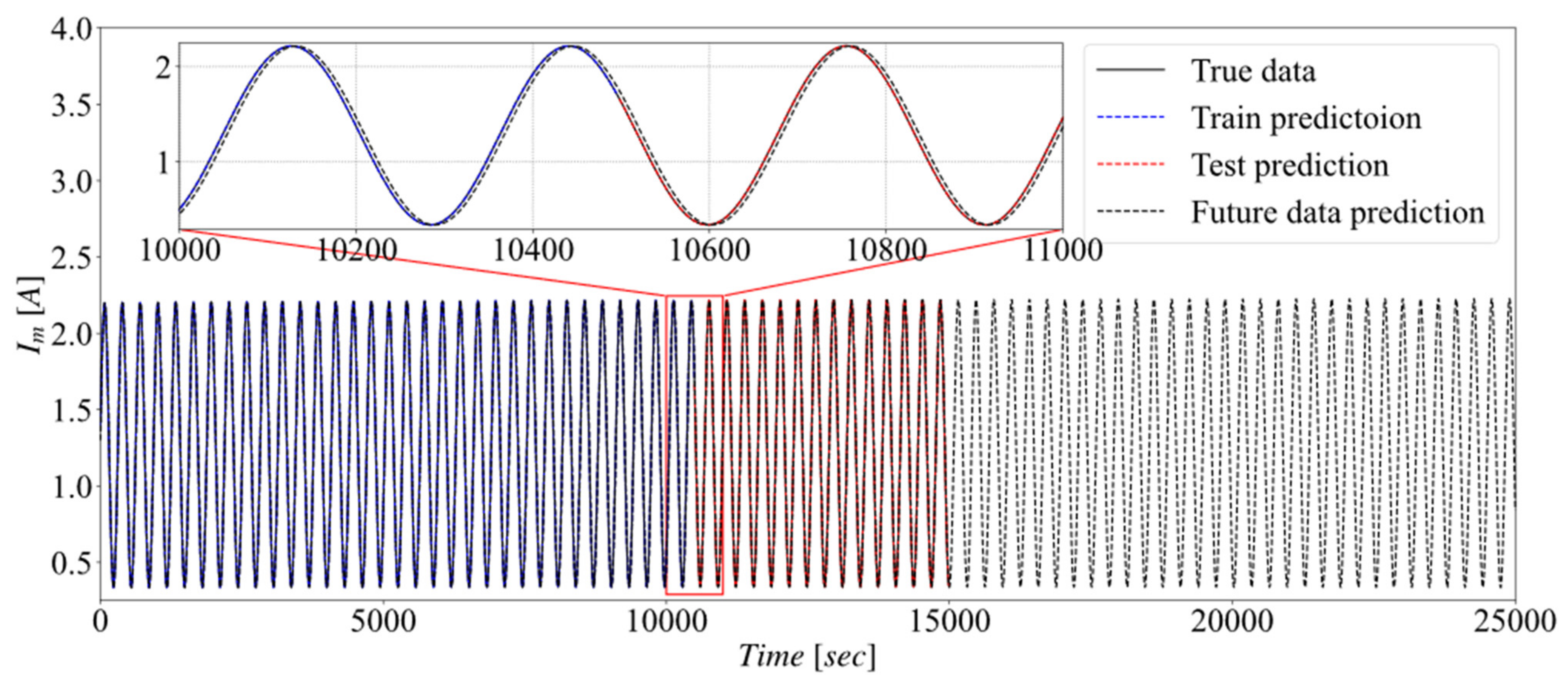
Figure 8 shows the prediction of motor current $(I_m$) data. As Figure 8 shows, the model almost accurately predicts the motor current. We obtain a NRMS prediction of 0.01 for motor current data.

Figure 9 shows the prediction of torque command voltage. The prediction in the Figure shows that it follows the true data in the test segment perfectly and can predict future data with considerable accuracy. We obtain forecasting accuracy of 0.01 NRMS for torque command voltage data.

Model parameters for the state prediction stage are listed in Table 2, where the final model characteristics after the tuning and validation are provided.

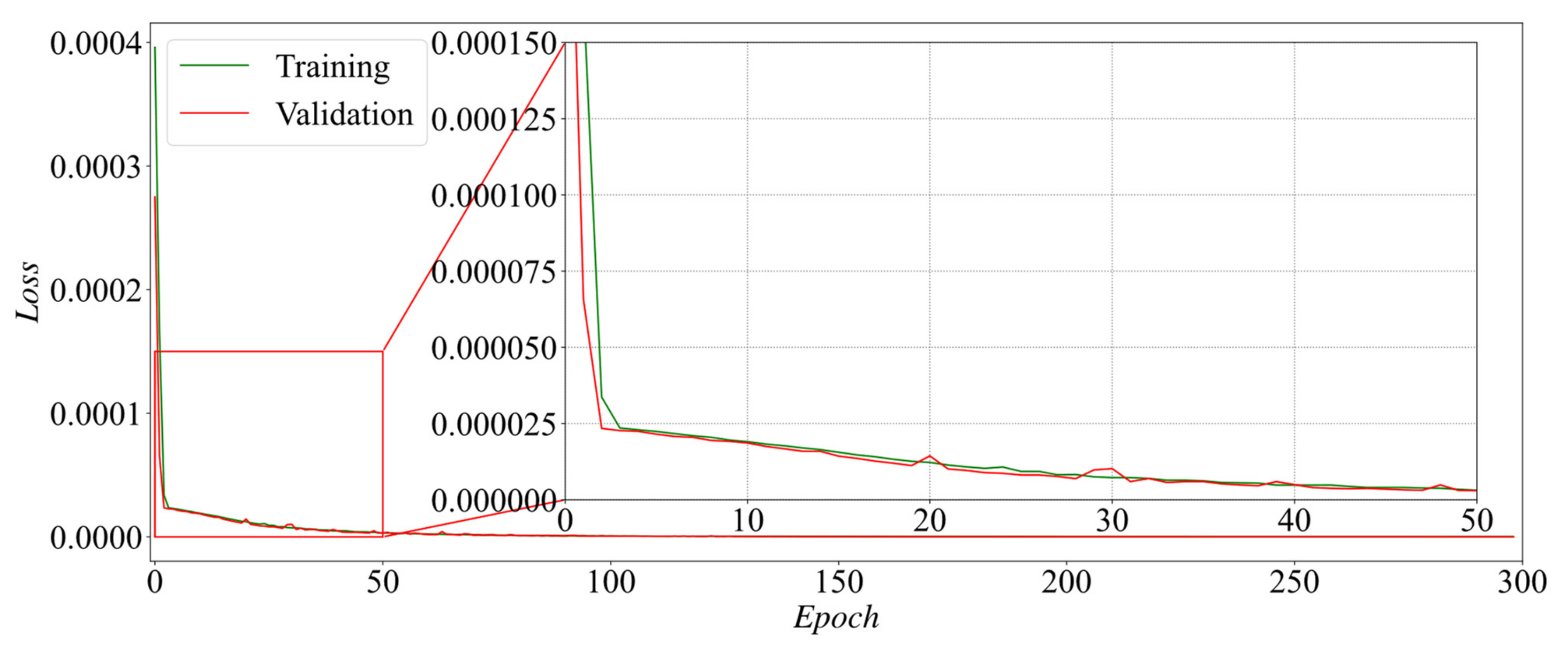
It is necessary to monitor the model’s loss to understand if the employed network learns the pattern for future prediction as necessary. We monitor the mean squared error loss calculated in the model training session (training loss) and the validation loss using validation data. The loss over time/epoch curves for the state prediction model are shown in Figure 10, Figure 11, and Figure 12. When comparing the training and validation loss trends over epochs, three cases can occur in machine learning and deep learning: (1) Underfitting, this is the only case where training loss is greater than the validation loss, but only slightly; if the training loss is far higher than validation loss, then there is some underlying issue with the model. (2) Overfitting is when the training loss is much smaller than the validation loss, and this means that your model is fitting the training data well but not at all the validation data; in other words, it is not generalizing correctly to unseen data. (3) Perfect fitting, when the training loss is more or less equal to the validation loss. If both values end up roughly the same, and if the values are converging (in the plot of the losses over time/epoch), then chances are very high that your model is trained correctly and working as intended. It can be seen from Figure 10, Figure 11, and Figure 12, that the training and validation loss curves overlap once the trend plateaus, which is a sign of behavior 3 from the three cases discussed above and satisfies the proper model for use.

The other observation from Figure 10, Figure 11, and Figure 12 is that the loss has plateaued after 50 epochs, which means additional epochs do not help improve the quality of the predictions by the trained model. Therefore, one can choose to stop the training and 50 epochs and expect to see the same results as the 300 epochs when the time required for training the model is an issue.

4.2. Parameter Prediction

Figure 13 shows the motor torque constant $\left(k_t\right)$ predictions. As Figure 13 shows, the prediction very closely follows the model-generated motor torque constant data. We obtain NRMS 0.02 for forecasting motor torque constant data. However, with the increase in time, there is a slight divergence from the true data. This happens because the uncertainty of the prediction increases with time.

Model parameters for the parameter prediction stage for hours span are listed in Table 3, where the final model characteristics after the tuning and validation are provided.

The loss over time/epoch curve for the parameter prediction model is shown in Figure 14. It can be seen from this Figure that the training and validation loss curves overlap once the trend plateaus, which is a sign of behavior 3 from the three cases discussed earlier, and satisfies the proper model for use.

The other observation from Figure 14 is that the loss has plateaued after 60 epochs, which means additional epochs do not help improve the quality of the predictions by the trained model. Therefore, one can choose to stop the training and 50 epochs and expect to see the same results as the 300 epochs when the time required for training the model is an issue.

4.3. Calculation of RUL:

In spite of the vastness of the universe beyond Earth’s atmosphere, a large number of human-made satellites are positioned in one of three orbital regimes: low Earth orbit (LEO), medium Earth orbit (MEO), and geosynchronous orbit (GEO). About 55% of all operating satellites are in LEO, and these satellites take 90 minutes and 2 h to complete a full orbit around the Earth. LEO satellites are ideal for remote sensing missions (e.g., Earth’s observation and reconnaissance) due to low altitudes and short orbital periods [43].

Therefore, in this section, three different time spans are covered, one in hours (~4 h) scale, one in days (~16 days), and one in months (~5 months) to show the performance of the proposed method over various time spans and life expectancy of the RW unit to make it more applicable to real-life applications.

4.3.1. Hours Span

For this simulation, the parameters in

Table 8. Parameters for hours span simulation.

Parameter/Function Name	Parameter Value/The Function
Data sampling rate	0.1 per second
Input frequency	0.1 Hz
Simulation duration	15,000 sec
$k_t$ incipient fault trend	$k_t=k_{t_0}\left(1/exp\left(t\times {10}^{-4}\right)\right)$

are used to inject the incipient fault in $k_t$ and record measurements at the identified speed. It should be noted that the fault injection trend is adjusted for each time span to ensure the data trend and degradation are meaningful for each simulation. If the fault injection for the hours span is used for the days or months span, the fault would degrade so quickly that at the span of days or months, it would only last within the first few hours, and the system would fail. Therefore, the speed of degradations has to be adjusted, as explained for each simulation according to the time span being simulated.

Figure 15 shows the confidence interval and a threshold line for the HI parameter to determine the RUL of the RW in the hours span simulation. The confidence is very narrow, and the model has a good prediction accuracy with NRMS of 0.02. However, it should be noted that, when predicting the future data, we predict based on the prediction of the previous time step. Therefore, the error is propagated even if there is a minor error in prediction. The prediction points out the system failure at 11,800 seconds from the beginning of the simulation, and the true data almost show the same failure time in the diagram. The threshold is drawn from historical data. At nearly 30 percent of the initial motor torque constant, the system fails to perform properly [1].

4.3.2. Days Span

For this simulation, the parameters in

Table 9. Parameters for the days span simulation.

Parameter/Function Name	Parameter Value/The Function
Data sampling rate	1 per second
Input frequency	0.01 Hz
Simulation duration	1,400,000 s
$k_t$ incipient fault trend	$k_t=k_{t_0}\left(1/exp\left(t\times {10}^{-6}\right)\right)$

are used to inject the incipient fault in $k_t$ and record measurements at the identified speed.

Figure 16 shows the threshold line for the HI parameter to determine the RUL of the RW in the days span simulation. The model has a good prediction accuracy with NRMS of 0.01. Comparing the results in Figure 15 and Figure 16, one can notice the difference between the true line and the predicted line has slightly increased to the additional time span simulated and its impact on the model predictions for the $k_t$ degradation and its corresponding RUL.

Model parameters for the parameter prediction stage for days span are listed in Table 4, where the final model characteristics after the tuning and validation are provided. With this model, the NRMS of 0.01 was achieved for the predictions.

4.3.3. Months Span

For this simulation, the parameters in

Table 10. Parameters for the months span simulation.

Parameter/Function Name	Parameter Value/The Function
Data sampling rate	two per second
Input frequency	0.0006 Hz
Simulation duration	13,200,000 s
$k_t$ incipient fault trend	$k_t=k_{t_0}\left(1/exp\left(t\times {10}^{-7}\right)\right)$

are used to inject the incipient fault in $k_t$ and record measurements at the identified speed.

Figure 17 shows the threshold line for the HI parameter to determine the RUL of the RW in the months span simulation. The model has a good prediction accuracy with NRMS of 0.02. Comparing the results in Figure 15, Figure 16, and Figure 17, one can notice the difference between the true line and the predicted line increases as the time span is extended. Particularly, comparing Figure 16 and Figure 17 shows that the deviation between the actual and predicted line has noticeably increased when moved from the days span to the months span simulation. This can be because, as the model relies more on the predicted data with larger time steps, its ability to predict future parameters correctly, given current and past data degrades.

Model parameters for the parameter prediction stage for months span are listed in Table 5, where the final model characteristics after the tuning and validation are provided. For this model, the NRMS of 0.02 was achieved for the predictions.

4.4. Sensitivity Analysis

To perform robustly in real-life applications, the model needs to perform under different conditions, including variations in missing data, noise, different input frequencies in the data, and data sampling rate. It should be noted that the results reported here are for the hours span simulations only due to space and time limits.

4.4.1. Missing Values

An interpolation technique is efficient enough for the proposed model to address the missing value issue, as shown in

Table 11. Missing data imputation accuracy for RW speed data.

Missing Value Ratio (%)	Prediction NRMS
5	0.01
10	0.02
15	0.02
20	0.02
25	0.04
30	0.05

.

4.4.2. Input Frequency

The accuracy of the model is measured in NRMS error for the test dataset. Table 6 shows that the model accuracy is better for RW speed prediction for higher frequencies and degrades for lower frequencies. However, for real-life applications, the use of much higher frequency has some complications. We have used an input frequency of 0.1 Hz for sensor data collection during other sensitivity analyses and RUL calculations.

4.4.3. Noise

Table 7 shows the model performance under the influence of added Gaussian white noise in the input data. As Table 7 shows, the model performance is very robust, and it can handle minor to medium noise in the input data without compromising the model accuracy. However, the model performance degrades with the introduction of higher noise levels in the input dataset. It should be noted that noise is added to each of the input data that is available from the simulations after the data are generated and before being fed to the model training for state and parameter prediction stages. The reported added noise strengths in Table 7 are in decibels, and each row lists the NRMS values for the test data for a combination of added noise strengths among all available measurements from the RW system, namely ${\omega }_m$, $I_m$ and $V_{comm}$.

5. Conclusions

This study proposed a three-step prognosis technique for calculating the RUL of the RW under incipient fault. A version of the recurrent neural network, LSTM, was used to predict future system measurements, also known as state reconstruction. Using a multivariate LSTM network, we predicted the RW health index parameter ($k_t$). From the failure threshold for the HI and its intersection with the HI predicted trend, we calculated the RUL of the RW. The proposed method was tested for robustness under noise, missing data, and different input frequencies. However, we carried out predictions based on the prediction in the previous time step when predicting the future data. Therefore, even a minimal error in prediction in the first step propagated to the next one, resulting in unsuiTable predictions over a longer time window.

The strength and novelty of the proposed method is that it is a new three-stage data-driven prognostic technique using LSTM, which is not complex with high computational costs and performs reasonably with accuracies achieved in the prediction of HI around 0.01–0.02 NRMS error, and the accuracy in prediction of RUL of 1–2.5%.

The limitations of the proposed method are as follows: we have considered one fault severity during our study, so there is provision for continuing the study to build a model that can address multiple types of fault scenarios at a time. Additionally, we have considered short and average operation lifespans in our simulations due to limitations in our computational and storage limits, where there is room for additional studies for more extended simulations and lifespans. Furthermore, we have considered the motor torque constant degradation as the HI for this study, where other factors can be additionally considered in building the degradation model and RUL prediction. Finally, our study introduced faults in the motor torque constant as an incipient exponential decline; however, other factors such as temperature changes, lubrication, and wear and tear can contribute to the overall reaction wheel system degradation.

The use of the proposed model can increase the reliability of the service by managing the scheduled maintenance time and reduce the possible downtime of the system with potential proactive measures. The proposed model has potential, as it provides a high accuracy RUL prediction method for reaction wheels that can be extended to other systems.