Article

Adequacy Evaluation of an Islanded Microgrid

Department of Energy Technology, Aalborg University, 9220 Aalborg Øst, Denmark
*
Author to whom correspondence should be addressed.
Electronics 2021, 10(19), 2344; https://doi.org/10.3390/electronics10192344
Submission received: 6 August 2021 / Revised: 9 September 2021 / Accepted: 16 September 2021 / Published: 25 September 2021

Abstract

:
The reliability of power converters has been extensively examined in terms of component- and converter level. However, in case of multiple generation units, the evaluation of the performance of power systems requires system-level modeling. This paper aims to merge the prior art of reliability modeling of power converters with the adequacy evaluation of power systems through an extensive design and evaluation analysis of a microgrid based case study. The methodology proposed in the paper integrates the device-level analysis into the domain of the conventional power system reliability analysis while outlining the steps needed to deal with non-exponential distributed failures of power electronic-based generation units. A replacement policy of the power electronic-based units is adopted by means of evaluating the system risk of not supplying system loads, and, finally, an approach on how to ensure a desired replacement frequency is outlined.

1. Introduction

Nowadays, power electronics constitute an essential part of the power system modernization, which is aimed at distributing electrical power, while leaving a low carbon footprint. Due to the indispensable role of power electronics in renewable-based power generation, the reliability of power electronics has a significant influence on the efficiency and cost of such systems, as elaborated in [1]. However, according to literature [2,3], power converters are among the frequent sources of failure in a wide range of applications, which can lead to an increase in downtime and maintenance related financial expenses. Additionally, according to field data, as power converters age, wear-out-related failures have a high tendency of occurrence, depending on the operating condition, as explained in [4].
The reliability of power electronic components depends on factors such as the device mechanical strength, applied electrical loading, the environmental conditions of its surroundings, and the applied control and switching schemes. These factors provide the basis for the physics-of-failure (PoF) analysis, the main concept of which is to understand how the elements of the converter react to various stresses and how these stresses affect the lifetime and degradation of the power converters, as outlined in [5].
The aforementioned reliability analysis is limited to the lifetime predictions of the power converter. However, in order to obtain optimal decision-making in regard to design, planning, operation and maintenance scheduling of power converters when integrated in power systems, power system analysis is needed to be conducted. This implies the need of bridging the concepts of converter reliability with the assessment methods used to evaluate power system reliability. The reliability of power systems on the evaluation of adequacy, i.e., is the generation capacity sufficient to satisfy the system demand when including the corrective and predictive maintenance of renewable-based generators [6]. Specifically, the ability of supplying system demand is measured by means of risk indices such as Loss of Load Expectation (LOLE) and Loss of Energy Expectation (LOEE), as explained in [7].
Considerable research has been conducted to gain insights in the optimum allocation of storage units and different types of distributed energy sources in order to optimize reliability [8]. In [9], energy management strategies are presented to increase the system flexibility by decreasing the variability between the distributed energy sources and the system loads, thereby increasing system reliability and resilience. In [10,11,12], research on control-based load curtail strategies are conducted, where non-critical loads are curtailed in order to provide continuous power supply to critical system loads. None of the existing literature covers the integration of physics-based converter lifetime expectancy into the concepts of power system reliability. This paper aims to integrate the non-exponential failure distributions of power electronic converters obtained in device-level analysis and introduce the concept of repair to compute the power electronic converter state probabilities needed for system adequacy analysis. Finally, this paper will also aim to adopt replacement policies of the power converters based on system risk evaluations analysis.

2. Approach

There are two major things that need to be considered when evaluating the power system adequacy, which are the probability of generation outage and what consequence this outage has on the system to perform in an adequate manner, as illustrated in Figure 1 [6]. These two concepts are examined separately throughout the paper and then later combined in order to evaluate the system risk. Initially, the system is designed in accordance with ensuring an adequate system when generator downtime is not considered. The consequence of an outage of each of the renewable generators are then examined by carrying out a mission profile translation, which takes into account the energy conversion efficiency and the limitations of each respective renewable-energy technology.
In terms of obtaining the probability of generation outage, the mission profile-based lifetime analysis of power converters needs to be carried out, which will result in the lifetime distribution of each converter-based generation unit. The reliability analysis of power converters has been researched and described extensively and will solely be outlined by the use of a methodology flowchart accompanied by brief descriptions and also including the suitable references needed for further study. The concept of repair is introduced, and the analysis moves into the power system analysis domain, where the additional techniques needed to cope with the non-exponential failure distributions are introduced, which is necessary for computing the state probabilities of the power electronic-based generation units. Finally, a replacement policy is adopted, which ensures that the system will not enter a state where inadequate operation is at risk.

3. System Framework

In this section, the system, which will form the basis for the analysis, will be described along with some modifications of the original proposed network in order to make it suitable for standalone reliability analysis. Additionally, the annual load demand and the intermittent renewable-based generation capacity, which is based on real-field environmental data, will be presented.

3.1. Network Type

A practical low-voltage benchmark system is modeled and used for reliability studies of fully renewable systems. The model is adapted from the proposed Cigre benchmark systems for network integration of renewable and distributed energy sources, which can be found in [13]. As the system has a high resemblance to an existing network, it can enable industry and academic research to perform a wide range of reliability-oriented studies of future power systems.
The Cigre low voltage (LV) residential network was solely designed for frequency regulation studies in case of short-term islanding mode, where the main source of supply under normal conditions was by means of a main feeder via a MV/LV transformer to upstream network. Due to most of the energy being supplied through an upstream network, during normal operation mode, it leads to a poor supply-and-demand ratio for long-term island-mode studies, as the supply contribution from upstream is no longer a considerable option. Since the overall purpose of this study is to perform long-term adequacy analysis of a standalone system, the Cigre LV benchmark system is modified with respect to its original form, and the final system used for the adequacy analysis is shown in Figure 2.
The system consist of 2 dual-stage photovoltaic (PV) inverters, one rated at 4 kW and one rated at 3 kW, and a wind-based generation unit with a back-to-back two-level converter topology, rated at 5.5 kW. Additionally, a storage unit of nominal capacity of 14 kWh is added in order to gain a degree of system flexibility by compensating for the intermittent energy production of the intermittent renewable energy (IRE) sources. It can be observed that the system presented in Figure 2 differs from the one proposed in [13]. The main purpose of the following sections is to describe which design modifications were made to the network in order to make the system fully adequate in a standalone operation, when generation outage is not considered.

3.2. Generation Capacity Overview

In order to evaluate the consequences related to an occurrence of generation outage, the real-field environmental profiles are needed to be translated into the available grid power. Obtaining the available power profiles consists of two fundamental steps in which one is to translate the environmental conditions into electrical energy by applying the energy conversion models of the respective IRE sources as well as to implement their respective limitations [14,15]. It is also needed to evaluate the conversion efficiency of the power electronic components at each power conversion stage. The concept is exemplified by means of the IRE technologies used in the system, as shown in Figure 3. In case of wind-based generation, the wind speed is correlated with the mechanical power applied to the generator shaft by the following expression [16]:
P m e c h = 1 2 ρ A v 3 C p
where v is the wind speed, ρ is the air density, A is the area swept by the turbine blades and C p is the wind energy utilization coefficient, which denotes to which extend the turbine is able to absorb and convert the wind energy. The wind energy utilization factor and the other relevant data of the turbine used in this case study can be found in [17]. In addition to the utilization factor, the turbine is assigned to an upper power level according to the manufacturer measurements, which can also be found in the referred manufacture datasheet. Finally, the lower limit, i.e., the power needed to overcome the mechanical friction of the permanent magnet synchronous generator (PMSG), also known as the slip-in speed, is needed to be taken into account. The machine parameters, which are available in [18], are applied to a full scale Piecewise Linear Electrical Circuit Simulation (PLECS) simulation model, which is controlled for at specified operating conditions of applied torque. The applied torque, which is sufficient to generate a power flow toward the grid, is translated into the slip-in wind speed.
In case of the solar-based generation units, the environmental profiles contain solar irradiance and ambient temperature, which are correlated with the output power of the PV array by the governing expression [19]:
i = I p h ( G , T ) I o ( T ) e v + R s i n N s V t h ( T ) 1 v + R s i R p
where I p h is the photo-generated current, I o is the dark saturation current of the PV module, R s is the series resistance, n is the ideality factor, N s is the number of series connected PV cells, V t h is the thermal voltage of a single cell and R p is the shunt resistance. Finally, the maximum feed in power is dictated by the amount of produced power by the PV arrays and the boost converter’s ability to track the maximum power point, as outlined in [20].
With the annual available power generated by the IRE sources obtained, it is now relevant to determine a demand and storage capacity, which ensures that the system is well qualified for adequacy analysis.

3.3. Unit Scaling

With the main goal of obtaining a system design, which is suited for standalone adequacy analysis, the system is required to be fully adequate when all IRE sources are in normal operation condition. This requirement is fulfilled by having a proper IRE generation capacity and load demand ratio. Previously, it was chosen to keep the ratings of the IRE sources, as proposed in the CIGRE benchmark system, and rescale the peak load so that a fully adequate standalone system is obtained. A daily loading profile was proposed to be used for studies of the system by the CIGRE task force [13]. Data points of the proposed loading profile, which CIGRE suggests using when analyzing the system, are extracted, and the loading profile is fitted and replicated by means of a sum-of-sines function and is presented in Figure 4.
i = 1 n a i s i n ( b i t + c i )
The rescaling of the peak load is approached in a simple deterministic manner, where the capacity and load ratio are based on having a spinning reserve equal to the largest rated generation unit in the system, as in [21].
In this particular case, the total rated generation capacity amounts to 12.5 kW with the largest generation unit being the wind-based generator with a power rating of 5.5 kW. Using these ratings results in a capacity load ratio of 1.44. As the largest unit (LU) method is originally meant to be applied for fully dispatchable generation units, some additional considerations are needed to be made. In case of IRE generators, the addition of their respective capacity factors along with the load factor is considered, which is simply the ratio of the actual annual energy production or demand and its respective rated values. Taking these capacity factors into consideration, with the aim of retaining the 1.44 ratio between total generation capacity and load demand, the values of system ratings presented in Table 1 are obtained.
The obtained capacity factors for wind and PV units are also presented in Table 1, which very much coincide with the historical data of real-field operating units [22,23,24]. It is worth noting that the system units can be scaled as desired as long as the ratio between generation capacity and load demand is maintained. Despite having an overall annual excessive generation, the intermittent nature of the non-dispatchable units creates a need to advance the system flexibility by the inclusion of a storage unit.

3.4. Storage Unit

In order to ensure a proper power balance of the grid, the surplus energy, which is not directly consumed by the load, is needed to be managed by including a storage unit. Battery energy storage systems are deemed as the promising solution due to the high level of scalability and the continuously significant decrease in battery unit cost [25,26]. Minimization of the cost of the stored energy is a crucial aspect in terms of ensuring the technology to be attractive and expanding the use of BESS in microgrids. The aspect of minimizing the cost of energy will eventually be a compromise of having sufficient nominal storage capacity to remove any possible deficit energy in the system power balance and not to oversize the unit, which will introduce an unnecessary high cost. A means to obtain an optimal sizing of the storage unit is based on gaining insights in the annual power balance in order to determine a common charging/discharging cycle length. Based on the most probable cycle length, the surplus and deficit distributions can be computed and the needed storage capacity can be determined. The power balance of the microgrid is computed as:
P b a l a n c e ( t ) = P w i n d ( t ) + P p v 1 ( t ) + P p v 2 ( t ) P l o a d ( t )
where P b a l a n c e ( t ) is the power balance of the system, P w i n d ( t ) is the power injected by the wind-based generator, P p v 1 ( t ) and P p v 2 ( t ) are the power injected by the two solar-based generation units and P l o a d ( t ) is the load duration curve shown in Figure 4. The resulting power balance is shown in Figure 5. As it can be observed in the figure, there is a pronounced deficit energy throughout the entire year, where the residential demand within the microgrid cannot be met by the IRE generation capacity.
The rainflow algorithm, which is explained in details in [27], is used to extract the cycle lengths of the power balance in order to gain insights in the charging and discharging time of the storage unit. From applying the rainflow algorithm, it is revealed that 93 percent of all power balance cycle lengths are covered within a time duration of three hours, both in terms of positive and negative valued cycles. The power balance profile is therefore reshaped into time intervals of three hours, and the surplus as well as deficit energy distributions within this time interval are computed, as shown in Figure 6.
As shown in Figure 6, choosing a nominal value of 14 kWh will ensure that 89.3% of all the surplus energy is stored. We also need to consider that it will require more than the double amount of nominal capacity to include the remaining 10.7%, as well as the fact that the deficit energy at no time exceeds a value of 7.5 kWh. A further increase in the nominal capacity will therefore lead to an oversizing of the storage unit, which will lead to an unnecessary increase in the cost of stored energy.
In order to minimize the cost in terms of long-term operation, a compromise of nominal capacity, power capability and lifetime needs to be made. The main stress factors of the unit, which directly influence the lifetime, are the depth of discharge, state-of-charge and the power capability [28]. The charging and discharging rates are already fixed based on the converter rating and will not be further elaborated. An ad hoc approach to lithium-ion-type batteries states that a good compromise between ensuring available capacity and battery performance is obtained by choosing the nominal c-rate, i.e., 1C, indicating that the unit is able to transfer all of its stored energy within one hour. At the same time, the unit should not be operated at low state-of-charge (SOC) levels because the battery voltage will decrease, leading to a compromised power capability. In this particular case, this is not expected to be an issue, when observing Figure 6 and considering that the nominal capacity is chosen well above maximum deficit energy levels and also considering the excessive amount of annual surplus energy with respect to the total amount of annual deficit energy. In [29], a correlation based on experimental results is developed between the cycle depth and the cycle capability. It was found that if the unit is not operated at SOC levels beneath 50% of full capacity, it will lead to the highest cycling lifetime. Finally, it is required that the capacity is sufficient throughout its entire lifetime, implying that the aging phenomenon known as capacity fade is taken into consideration. Usually, the end-of-life criterion for batteries is when its nominal capacity reaches a value corresponding to 80% of its initial value, as the rate of degradation severely accelerates when exceeding this capacity fade value [30]. With the aim of storing an efficient amount of energy to remove all deficit energies from the system, while also considering the stress and aging mechanisms, the initial nominal capacity of the battery at its beginning of life is required to satisfy the following constraint:
C n o m i n a l , B O L · Δ D O D 1.25 E s u r p l u s
where Δ D O D is the depth of discharge, which is shown to reduce to 1, in [30], if the unit is not operated at SOC levels beneath 50%. E s u r p l u s is the initial chosen capacity size of 14 kWh, and the factor of 1.25 reflects that a sufficient capacity is obtained when also considering a capacity fade of 20%, which results in a nominal capacity at beginning of life of 17.5 kWh. Limiting the charging and discharging power according to the converter rating, i.e., 5.5 kW, and limiting the nominal capacity to 17.5 kWh result in an annual state-of-charge profile, as shown in Figure 7.
Finally, the annual storage capacity is obtained based on the design considerations outlined in Section 3.4. As it can be observed in Figure 7, the unit is mostly operated at a state-of-charge region between 50% and 100% of full capacity, which enables a high cycle lifetime of the unit due to not being based on the common mode of operation on high levels of discharge states. Finally, the descending values of the state-of-charge profile are extracted, i.e., the discharging profile, and are added to the power balance without added storage capacity, as shown in Figure 5. Adding the storage capacity to the system results in the power balance shown in Figure 8.
It can be observed that any deficit energy presence from the annual power balance without storage is removed by adding the designed storage capacity, and the microgrid is thereby fully adequate during failure-free operation. Now that the system design is carried out, it is relevant to include the likelihood of generation outage, which requires a comprehensive reliability analysis of the power converters.

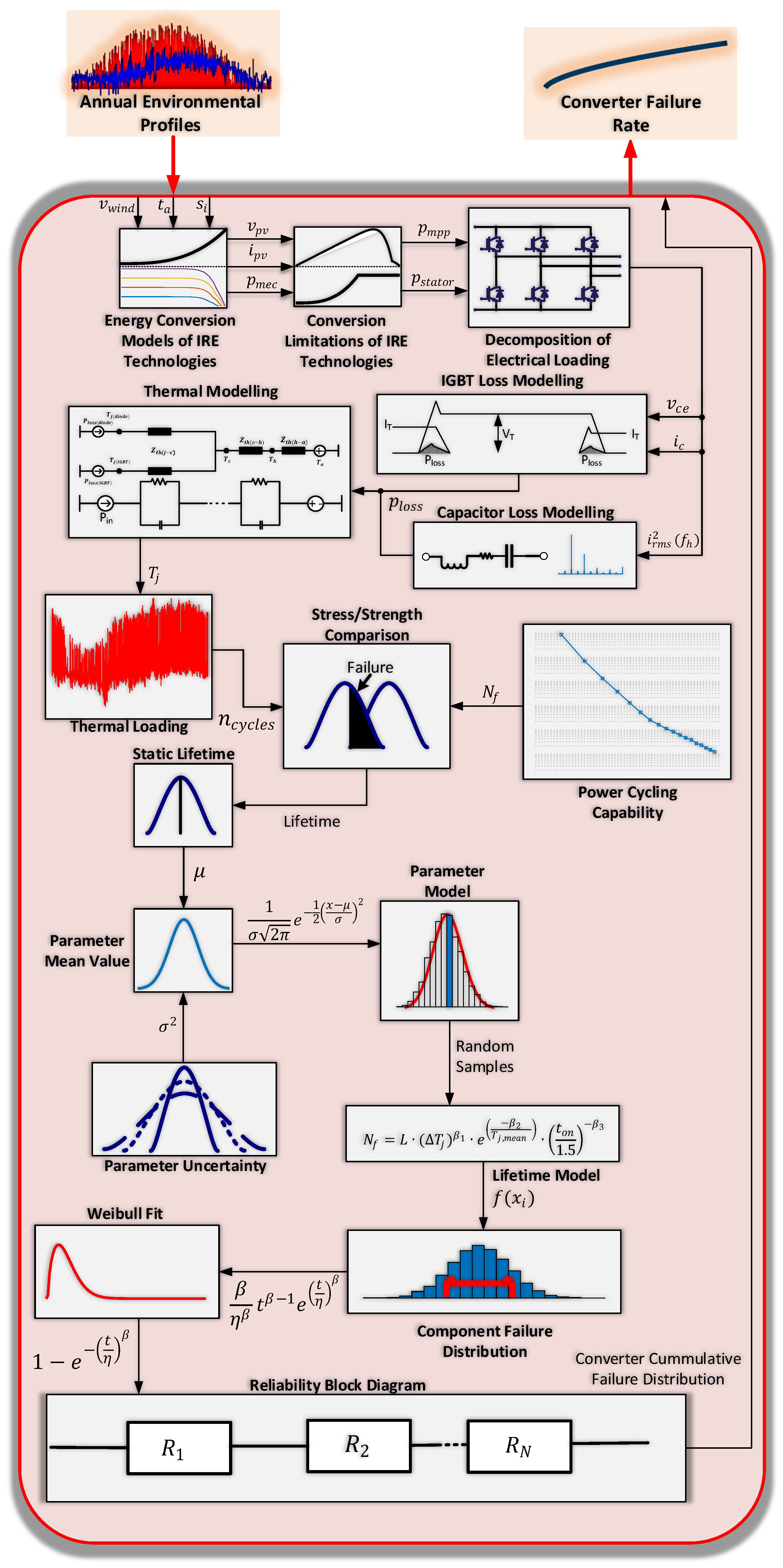
4. Obtaining Converter Failure Distributions

The mission of profile-based lifetime estimation analysis is an exhaustive process, which has been thoroughly described in the existing literature [31,32,33,34,35]. The process will therefore only be described on a basic level by means of mentioning the key steps accompanied by a graphical representation of the entire process, as shown in Figure 9.

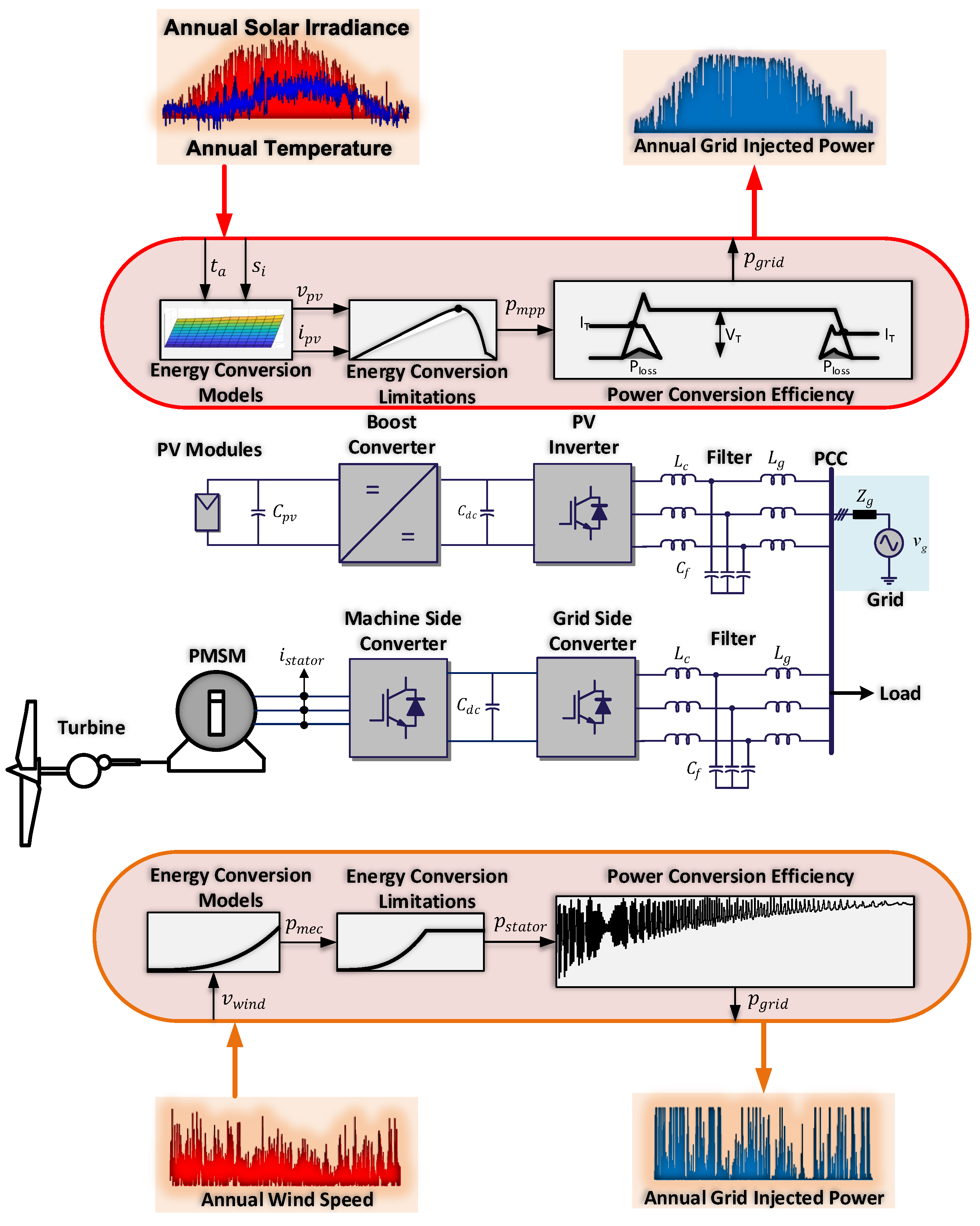
4.1. Loading Translation

Each of the power electronic components are exposed to different critical stressors, where one of the main life-limiting stressors are temperature-related stressors, which affect the reliability of several components in the power electronic systems. Components such as capacitors and semiconductors are both influenced by the temperature subjected to each.
In terms of semiconductors, the stress is mainly related to both the average junction temperature and the junction temperature cycling and can be further divided into that evoked by ambient temperature and one that is the component’s self-heating, which is also known as power cycling [36].
The wear-out present in power electronic converters is caused by changes in the materials, and the presence of current variation causes the different elements, which inhibits different temperature coefficients from expanding unequally due to thermal stresses. The materials will change continuously in accordance with the loading profile, which eventually will lead to fatal component failures. It is therefore of high importance to know the real loading profile subjected to the power converters [37]. This implies that it is fundamental to obtain the correct amount of power, which can be utilized from the renewable energy sources, which then can be translated into the thermal loading of the components. In terms of obtaining the thermal loading subjected to the reliability-critical components, the environmental profiles are translated into electrical or mechanical loading by means of the energy conversion models of each respective IRE technology by use of characteristic models [16,19]. The available power subjected to the photovoltaic inverters is obtained by considering the MPPT operation efficiency, whereas the power supplied to the wind-based power converters is obtained by considering both the power sufficient to rotate the turbine and the power saturation obtained at rated speed.
The obtained dissipated losses are applied to a thermal model of the power devices, which provides the junction temperature T j , i.e., the thermal loading for the given operation. Similarly, the power losses dissipated in the capacitors can be obtained by considering the dc-link ripple current subjected to the equivalent series resistance (ESR). More detailed descriptions of the mission profile translations of power devices and capacitors can be found in [14,34,38,39,40], respectively. For long-term simulation, some well-suited operating conditions are defined, and the corresponding conduction and switching losses along with the thermal impedance of the power device are inserted in look-up tables, assisted with the interpolation method of choice [41,42].

4.2. Categorization of the Thermal Loading

The thermal loading of the components, for some given operational profiles, was obtained by the methodology previously described. In the case of the power devices, the most likely failure mechanisms are often a consequence of the continuous variation of the thermal stress, which is applied to the interconnections between the device and the external contacts of the power device. The long time effect of the power cycling leads to degradation of the interconnection between the bond wires and the solder layers of the power devices [43]. In order to evaluate the chance of these particular failure mechanisms’ occurrence, information of the thermal cycling is needed, e.g., the number of cycles contained in the profile n i , all of which have a certain cycle amplitude, Δ T j , a mean temperature, T j , m e a n , and finally the cycle duration, T o n . This information is not directly available from the junction temperature profile due to its irregular dynamical nature. In order to categorize the dynamical profile into the above-mentioned quantities, a counting algorithm is needed, which, in this case, is realized by the use of rainflow algorithm. The main function of the algorithm is to decompose the irregular profile into a number of regular cycles, which can then be classified in terms of variation amplitude, mean value and cycle duration. These regular cycles can then be directly applied to the strength models of the components [44].

4.3. Strength Models of the Components

With the annual stress at hand, it is now relevant to model the strength of the power electronic components, i.e., how many cycles each of them can withstand. The lifetime can then be estimated based on a comparison of the applied stress and the component strength, as shown in Figure 9. With respect to field experience, it is revealed that the converters are one of the most critical sub-systems in terms of failure rate, lifetime and maintenance cost, and that there are several of the power converter components that can induce system failure [45,46]. The wear-out of some components might even influence the reliability of others, which would result in a very exhaustive and complicated analysis. Due to the power devices and capacitors being identified as the most failure-prone and therefore the most life-limiting components of power converters, they are solely taken into account in this paper when considering the wear-out of the power converters [2,37].
The analytical lifetime model of the power devices are based on fitting experimental lifetime data containing the main factors, which influence the lifetime. The lifetime model parameters used in this paper, which describes the power cycling capability of power devices, are based on the testing data provided by a leading power semiconductor manufacturer [47]. The three quantities relating the number of cycles to failure are the temperature cycling amplitude Δ T j , the mean junction temperature T j , m e a n and the heating time T o n . A commonly used model, which accounts for the quantities mentioned above, is the extension of the Coffin–Manson Model, which can be expressed as [48]:
N f = α ( Δ T j ) n exp E a K T j , m e a n t o n 1.5 β
where K denotes the Boltzmann constant; E a is the activation energy; and the parameters α , n and β are obtained from fitting the testing data curves presented in [47]. The lifetime estimation is based on the accumulation of damage caused by each of the cycles contained in the annual stress profile, as shown in Figure 9. A widely used assumption is the linear damage accumulation, which is known as Miner’s rule and which can be expressed as [39]:
A D = i = 1 n n i N f , i
where n i is the number of cycles of the ith stress level and N f , i is the corresponding number of cycles until the end-of-life. When A D = 1, the end-of-life is reached and the estimated lifetime can then be obtained as the reciprocal value of the accumulated damage.
In the case of capacitors, the main stress factors are the operating voltage V o and the hotspot temperature T h . Applying the annual stress profile, the lifetime can be estimated by the lifetime model, which is given as [49]:
L f = L 0 · V V o p 1 · 2 T o T h p 2
where L o , V o , V, T o and T h are the rated lifetime, rated voltage, applied voltage, rated temperature and hotspot temperature. For the electrolytic capacitors, the parameter denoted p 1 is usually in the range of 3–5, whereas the parameter p 2 is often at a value of 10 [49]. For long-term operating conditions, the Miners rule can be applied
D = i = 1 n l i L f , i
where n i is the number of cycles of the ith stress level and N f , i is the corresponding number of cycles until the end-of-life.

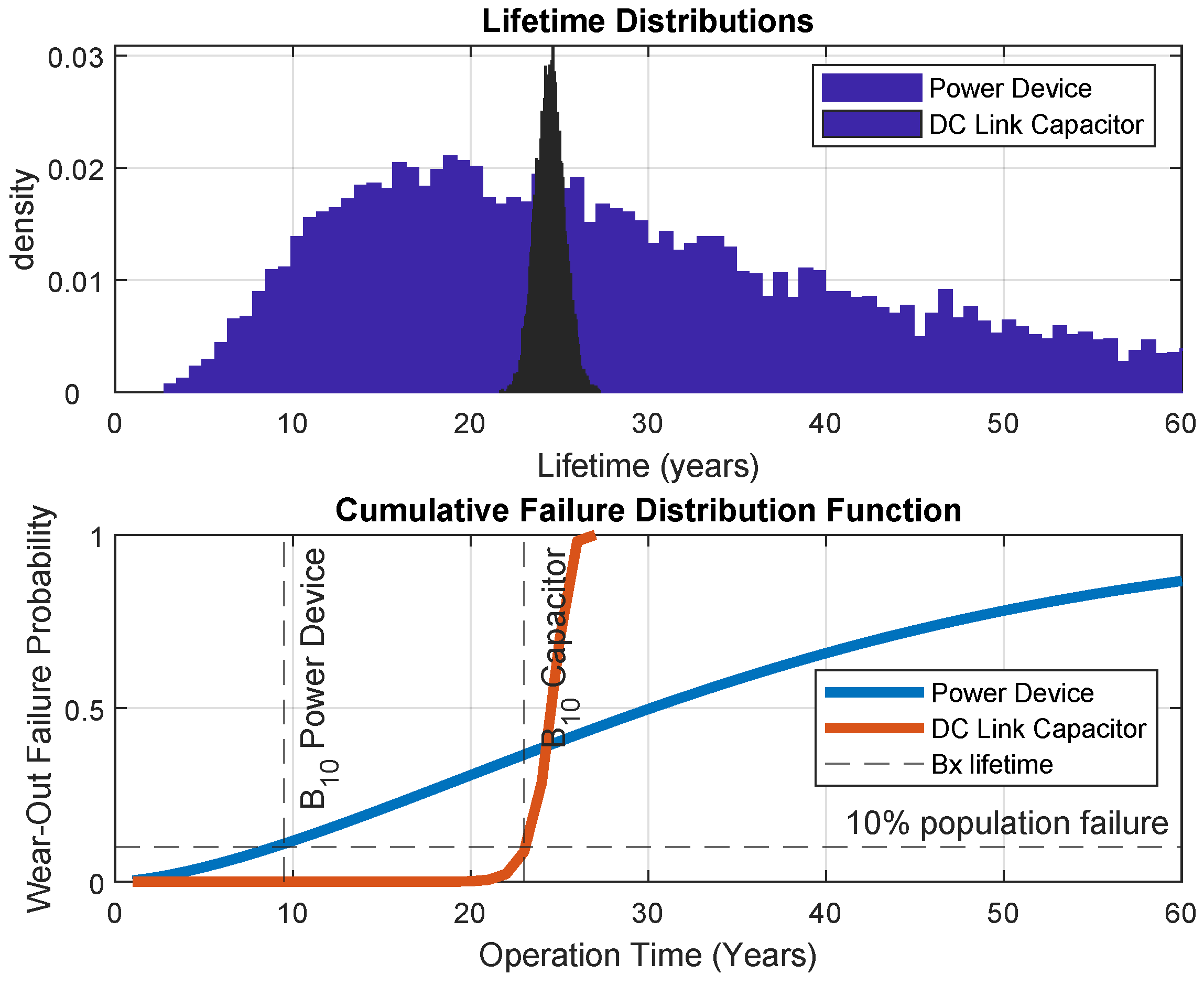
4.4. Component Variation and Weibull Analysis

Uncertainty needs to be taken into account as the parameters of the lifetime model will vary at different testing and operating conditions. The electrical parameters of the components can also differ due to variations in the manufacturing process and, lastly, the applied stress to components can also vary on a year-to-year basis due to climate variations. Due to these uncertainties, the reliability assessment on component level needs to be based on Monte Carlo simulation, where the main aspects are to model the parameters used for lifetime estimation as distribution functions with carefully chosen variance. Carrying out the Monte Carlo simulation will result in a lifetime distribution of each components, which will in turn result in a more realistic lifetime measure compared with those based on static lifetime values, as it is very unlikely that components will fail at the exact instant [34,50,51,52]. In terms of the lifetime model parameters, the static equivalents of the stress variables are initially determined as the static values, which would produce the same amount of lifetime consumption, which was obtained by applying the annual stress profile given as:
N f , i = N f , s t a t i c = α · ( Δ T j , s t a t i c ) · e E a k b · T j , m e a n , s t a t i c · T o n , s t a t i c 1.5 β
The lifetime model parameters α , n and β are then modeled as distribution functions with the model parameters determined in [53]. The lifetime evaluation is then carried out according to the approach described in Section 4.3 with a population of n amount of samples, which will constitute the lifetime distribution. The Weibull distribution function is fitted with the resulting sample lifetime yield, which can be expressed as [4]:
f ( t ) = β η β t β 1 e t η β
An example of the obtained results from the Monte Carlo simulation, showing the lifetime yield of a power device and a dc-link capacitor of the wind-based generator, is shown in Figure 10.
It can be observed in Figure 10 that there is a significant spread in the failure distribution of power devices, whereas the entire capacitor population will fail within a time span of 5 years. This is also obvious from the slopes of either cumulative distribution functions, which describe the evolution of failure, where the rate of change for the capacitor failure is significantly higher. The function is suitable for use as a reliability metric in terms of an allowable failure percentage, which is normally referred to as B x lifetime [4]. The B 10 lifetime for a power device and a dc-link capacitor operating in the wind-based generation unit are 9.5 and 23 years, respectively, as depicted in Figure 10.
Finally, the obtained reliability of each individual power electronic component can be combined in order to obtain the Weibull failure distributions of entire generation units, e.g., the PV-based unit or the wind-based unit, each of which contains several power devices, diodes and capacitors. The reliability of these systems is assessed by the use of the reliability block diagram (RBD), and the combination to obtain the equivalent distributions is dictated by how an individual component failure will affect the system’s ability to operate. For a system with n components, where one single failure of any of the components will cause the overall system failure, the system is considered to be a series connection of the reliability block diagram [4].
R ( t ) = i = 1 n R i ( t )
If, on the other hand, the system only requires one of the system’s components to operate for satisfactory operation, it can be considered as active parallel redundancy, in which the reliability of a system as such can be expressed as [4]:
R = 1 i = 1 n ( 1 R i ( t ) )
When the distribution of each generation unit is obtained, the failure rate can be obtained, which is a fundamental requirement when moving into the power system domain reliability analysis. The failure rate can be calculated by the use of the fitted Weibull shape and scale parameters of the generation unit failure distributions as [4]:
λ ( t ) = f ( t ) R ( t ) = β t β 1 η β
where the obtained shape and scale factors of each respective generation unit are presented in Table 2.

5. Availability Modeling of Power Converters

One fundamental requirement of power systems is that they must be able to operate at all times. This implies that a fundamentally different approach is needed, as we are moving into the power system domain, compared to the ones used for converter level analysis in Section 4. This is due to the fundamental difference between how repairable and non-repairable systems are treated mathematically. None of the commonly used distributions used for converter level analysis can be applied to repairable systems due to the fact that they assume that the repair time is instantaneous, which, in this case, is not a valid assumption [54]. Instead, the power system reliability should be modeled as a stochastic process. In this case, the converters are considered to be replaced whenever they enter a repair process and can therefore be considered to be in a “as good as new” state at the end of the repair process. This consideration is the most likely case when considering the cost of unit downtime, where the long and exhaustive process of locating and remedying any particular defect is highly unlikely. Moreover, for a repairable system, the “classic” definition of reliability will only be rightfully applicable until this first unit failure occurs. Instead, the reliability-equivalent of power systems is known as availability, which is defined as the probability of the unit being available, i.e., the proportion within a finite time interval, where the generation unit is available for operation [54]. The availability is evaluated by its failure rate λ and its repair rate μ , which can be used to evaluate the steady-state availability for constant transition rates given as [21]:
A = μ λ + μ
The stochastic nature of power system reliability can be modeled by the use of the Markov approach, but needs some extension methods in terms of incorporating the non-constant failure rates inhibited by the power electronic converters. Applying the non-constant failure rates obtained in Section 4 results in a non-stationary process, i.e., the probability of making a transition from one state to another does not remain the same at all times [55,56]. The repair rates, on the other hand, are considered to be constant for the sake of simplicity. The repair rates are based on the assumption of 2-day repair time due to the easy accessibility of converters operating in a residential area. For offshore wind farms or units operating in other remote areas, the repair time must be considered to be longer.
In order to aid the solution of the availability of the power electronics-based generation units, it is desirable to construct the appropriate state-space diagram of the system. The state-space diagram outlines all the states in which the system can reside, while also showing how transition between the system states can occur. Including the state space diagram is an important part of the reliability assessment, as it translates the knowledge of the system operation into a mathematical model, which can be solved using the Markov techniques. Considering that each generation unit can exist in either down or operational state and that only one event can occur from one state to another, the state-space diagram shown in Figure 11 is obtained based on the network shown in Figure 2.
As shown in Figure 11, all unique states are defined and linked by their respective failure and repair rates, and the number of states contained in the state-space diagram increases with the number of power electronic converters operating in the system with the rate of 2 n for an n-converter system. A model describing each state by an analytical expression will therefore be impractical and unmanageable for systems of this size, also considering that this method is desired to be scaleable to larger systems. There are two solutions to overcome this issue. One method is to use state truncation by neglecting the states, which has a very low probability of occurrence. The other method, the one used in this research, is based on utilizing the stochastic transitional probability matrix to evaluate the individual state evolution through time by containing all the possible transitions that can occur in the system. This tool is used in the case of discrete Markov chains and, as we are concerned with power electronic transition rates and not transition probabilities, i.e., continuous Markov process, a carefully chosen incremental of time Δ t is to be defined. As shown in Figure 11, one of the fundamental assumptions utilizing this particular approach is that, at any transition to another state, only one event can occur, e.g., in the transition from state 1 to state 2, where only one converter has changed its condition from being operating to being down. This implies that the introduced time interval needs to be chosen to be short enough in order to ensure that the occurrence of two events happening within this time interval is highly unlikely. In this particular case, the incremental time interval was chosen to be 1 h, since it is highly unlikely to have downtime of two converters simultaneously within this particular time span. Including this interval results in the matrix entries taken on discrete form as (16), which enables the use of the stochastic transitional probability matrix:
p = λ Δ t
P = P 11 P 12 P 13 p 1 n P 21 P 22 P 23 P 31 P 32 P 33 p m 1 p m n
Where the row entry of the matrix denotes the state from which the transition occurs and the column entry denotes the state to which the transition occurs. The evaluation of the transient behavior of the converter state probabilities is computed by raising the stochastic probability matrix to the power of the desired number of time intervals by use of iteration.

Incorporating the Non-Constant Failure Rates

As explained in Section 5, the conventional Markov approach explained up until now only applies for the stationary processes, i.e., for constant failure rates. The inclusion of the uncertainty and the Weibull analysis, described in Section 4.4, have resulted in non-exponential failure distributions and thereby non-constant failure rates. This implies that additional techniques have to be added to the method already presented. There are several techniques available to cope with non-exponential distributions [57,58], and the one used in this research is based on dividing the existing system states into sub-states, each of which is exponentially distributed.
The essence of the following is to outline how to obtain the numbers of sub-states, which is required, how the sub-states should be configured and which parameters should represent them. In the case of Weibull distributed failures with an increasing slope, i.e., β 1, each existing state can be divided into a number of series-connected sub-states, as shown for state 1 in Figure 12. The bathtub curve is shown in Figure 12b, which is a superposition of each failure type a power converter can encounter throughout its operational lifetime.
The curve shows an initial decreasing failure rate also known as the infant mortality period, an intermediate useful life period and the final wear-out period. The periods considered in this case are the useful life and wear-out stages, where the failure rate is either constant or increasing. The increasing failure rate of the power converters are modeled by decomposing the failure transition of each of the system states shown in Figure 11 into a number of identical exponential distributed states with transition parameter p [58]. The probability function takes on the form of the special Erlangian distribution when all states are identical and their respective state duration can be described by exponentially distributed variables. The special Erlangian distribution can be expressed as:
f ( t ) = ρ ( ρ t ) α 1 e ρ t ( α 1 )
for which the r t h moment is given by:
m r = 1 ρ r k = 1 r ( α + k + 1 )
The decomposed state has two parameters, α and ρ . The numerical values for these parameters, the first and second moments of the special Erlangian distribution, are to be matched with the corresponding moments of the Weibull distribution of the converter failures. The first and second moments of the special Erlangian distribution can be calculated by letting r = 1 and r = 2 in Equation (19), which leads to the following:
m 1 = α ρ and m 2 = α ( α + 1 ) ρ 2
Now let M 1 and M 2 be the respective first and second moments of the Weibull distributions describing the failures of the converter-based generation units and requiring the moments of each of the distributions to be equal to each other:
m 1 M 1 = 0 and m 2 M 2 = 0
Substituting the two expressions for the Erlangian moments in (20) into the two expressions in (21) and then isolating for α and ρ , respectively, it leads to:
α = M 1 2 M 2 M 1 2 and ρ = M 1 M 2 M 1 2
where α is the equivalent number of exponentially distributed states the original state is required to be decomposed into and ρ is the transition rates linking the exponentially distributed states. The two parameters in (22) are now a direct function of the shape and scale parameters of the Weibull failure distribution, which can be obtained as:
M r = η r · Γ 1 + r β
For the sake of examining the effect of including the non-constant failure rates when evaluating the state probabilities, the probability of all converter-based generation units is computed with the use of both constant and non-constant failure rates, as compared in Figure 13. In the case of constant failure rates, the use of each static lifetime of the converters are used:
λ c o n s t a n t = ( Static lifetime ) 1
As it can be observed, the transient state is significantly prolonged when modeling the non-constant failure rates. It can also be observed that the use of constant failure rates will overestimate the system downtime during the first half a year but will severely underestimate the downtime in long-term operation, thereby underestimating the system risk. Basing the risk evaluation of power electronic-based power systems on constant failure rates will therefore not lead to valid results and should be avoided.

6. Risk Evaluation

The aim of the following is to develop a replacement policy of the converters, which will ensure an adequate IRE-based power system. The replacement policy will be based on defining an allowable system risk that cannot be violated at any time. As previously mentioned, risk is a combination of the probability of generation outage and the resulting negative consequences an outage of that particular extent will cause [6]. The negative consequences of losing any of the generation capacity contained in the annual power generation profiles are obtained by the methodology described in Section 3.2. The development of a risk criterion with one single quantitative measure is seldom used, as any decrease in system risk is always linked to a certain cost, which should therefore be evaluated if any decrease in risk is cost beneficial. Due to the vague distinguishing of acceptable risk from unacceptable risk with a straight quantitative measure, the risk is instead divided into three zones of acceptable small risk, tolerable risk and unacceptable large risk, as illustrated in Figure 14. The decrease in risk within the tolerable risk zone is only desirable if it is practical and cost beneficial, and evaluating this is a complete analysis on its own terms and is out of the scope of this paper.
The index, which is used to evaluate the system risk, is designated as the loss of load expectation (LOLE), which can be expressed as:
L O L E = i = 1 n P i ( C i L i )
where C i is the available capacity at time step i, L i is the load demand at time step i and P i is the probability of a generation outage causing the corresponding amount of loss of load. In other words, one specific capacity outage will contribute to the system LOLE by an amount that is equal to the product of the probability of this particular outage’s occurring and the number of time steps covered within the interval that loss of load would occur, if such a capacity outage would exist.
The most convenient method to evaluate the system LOLE would be to compute the product of the overall unavailability of the system, as shown in Figure 13, and the difference between the total generation capacity and load demand. This would not produce realistic results due to not taking into consideration how this unavailability is divided into the individual units, which would thereby result in obtaining misleading risk rates. Instead, the unique states of each individual generation outage should be considered along with their corresponding negative consequences. On the other hand, for this particular case, only the four unique states of single unit outage are considered, as the limiting state probability of two or more IRE generation units being down simultaneously is in the order of 10 6 and therefore does not contribute to the system risk in magnitudes worth considering. It is also worth mentioning that it would lead to inaccurate results if the LOLE evaluation is based on using the generation capacity distributions along with the resolution of the profiles, as this will not take the uncertainty of intermittent production into account. That is to say, it does not take the exact time into account, and the majority of a unit outage could be at a time when it is actually not needed in order to make the system fully adequate. Instead, each unique outage state should be realized by removing the corresponding generation capacity profile from the system power balance and obtaining the total time duration of when the loss of load occurs by the number of deficit values and the profile resolution.
We should consider evaluating the system LOLE while adopting an allowable risk limit of 10 h per year. Not exceeding a system LOLE of 10 h per year is generally considered as a reliable power supply and is used in the majority of European countries, where the limit is settled between 5 h per year and 10 h per year [59]. By means of the previously stated methodology and by computing Equation (25), the system risk is evaluated, as shown in Figure 15.
As the converters age, the probability of them entering a failed state increases, which is reflected in the risk of not supplying the system load, as shown in Figure 15. As the system LOLE is the sum of the contribution from each individual IRE unit, a replacement policy of each is based on not violating the system risk limit, which will result in the individual converter replacement policy, shown in Figure 16.
As it can be observed in Figure 16, at the time of replacement for any of the respective units, the risk induced by them resets, which ensures that the risk of losing the system load will not exceed 10 h per year. In order to gather an understanding of how much of the total energy demand is met when adopting this particular replacement policy, the energy index of reliability is computed as [55]:
E I R = 1 L O E E n o r m a l i z e d = 1 k = 1 n E k P k E t o t a l
where L O E E n o r m a l i z e d is the loss of energy expectation normalized with respect to the total energy demand, which represents the ratio between the probable energy curtailed due to converter-based generation down time and the total energy required to satisfy load demand. Adopting the replacement policy shown in Figure 16 amounts to the percentage of load demand met, shown in Figure 17.
As it can be observed in Figure 17, this leads to the probability that the load demand will not be met, which will never exceed 0.2 percent. As it can be observed in Figure 16, the frequency of replacement of the units is relatively high, which is a direct consequence of the power electronic components and their respective stress and strength margins chosen for this particular study. One method that can ensure that the desired replacement times for a given application is met is incorporating the design for reliability aspect. Incorporating this aspect is out of the scope of this paper, but it is still worth suggesting as an applicable methodology. The main idea is to reinforce the components in terms of rating margins with respect to how the units are operated throughout their operational lifespan. This reinforcement is carried out until a desirable frequency of converter replacements is obtained, as depicted in Figure 18.
As shown in the figure, it is not needed to carry out all of the outlined steps of this paper, if some knowledge is obtained of how much the converter B 1 lifetimes translate into a certain time of replacement. Reinforcing the components will result in lower frequent replacements while maintaining a low system EIR. It is also worth noting that the system reliability is never more reliable than its weakest link, and reducing the rate of risk induced by the most unreliable units will be reflected in the replacement frequency of all of the system units.

7. Discussion and Conclusions

Extensive studies have been carried out in regard to assessing the reliability of power converters. However, power electronics constitutes a substantial part of renewable power generation and, due to its indispensable role within power systems, it has a significant influence on the overall performance of the system. Due to the requirement of the power systems to operate at all times, the power converter reliability analysis needs to be extended in terms of introducing the concepts of repair and their respective availability. There is therefore a need to merge the reliability assessment of power converters with the conventional power system reliability concepts. One of the main measures in the power system reliability assessment is the concept availability of the generation units, as power converters inhibit non-exponential failure distributions, which are not applicable with conventional availability modeling. This paper proposed a method to extend the reliability assessment of power converters, which enables to analyze them when they are operating in power systems. The method proposed also outlines a technique that enables to incorporate the non-exponential failure distribution of power converters, which still makes use of the conventional Markov process modeling, enabling the adequate evaluation of the distributed generation systems.
The conventional methods of analyzing converter systems are based on combining the individual failure distributions by use of reliability block diagrams. Utilizing the conventional methods is based on assuming that the repair process is instant, which does not coincide very well with the nature of real systems. To take into account the repair process, the concept of generator availability was introduced. Availability modeling becomes a tedious affair when considering systems with a considerable amount of units and, in particular, when these units do not inherent identical and constant failure rates.
The method of discretizing the continuous Markov process, by carefully defining a time interval, wherein the occurrence of two, or more, state transitions are highly unlikely, converts the problem into one that can be analyzed as a Markov chain. One of the common techniques used for the computation of state probabilities of Markov chains is the stochastic transitional matrix, which has some significant computational advantages compared with those methods, which makes use of analytical expressions. In regard to semi-Markov processes, they require the evaluation of complex convolution integrals, and when exceeding three non-identical units, the method of obtaining conventional Markov expression becomes rather tedious. Additionally, the use of the stochastic probability matrix has a clear advantage in terms of scalability when performing the adequacy analysis of power electronic-based power systems, as this simply requires an increase in matrix dimension, and does not require solving large systems of equations, which will simply result in complicated expressions, and which are unsuited for further analysis. Utilizing the Markov chain techniques in combination with decomposing the non-constant failure rates ensures a relatively simple method when evaluating the availability of the system units.
Lastly, a replacement policy of the power converters guarantees that the system is being operated without entering a state of being at risk of being inadequate. The failure nature of power converters leads to a highly frequent replacement in order not to cause excessive system risk. The issue of frequency replacements of power converters can be met by reinforcing the power electronic components by reconsidering the design and strength margins with respect to their operational conditions. The process of redesigning the components is an iterative process that is carried out until a reasonable percentage of component population failure is reached. Gaining a desired component population failure will influence the replacement policy frequency of the power electronic-based generation units, while maintaining a reliable and adequate power supply.

Author Contributions

Conceptualizing, all listed Authors; Methodology, M.K.; Computations and data processing, M.K.; Validation and Encouragement to investigate, H.W.; Writing and preparing, M.K.; Supervision, H.W. and F.B.; Project administration and funding acquisition, F.B. All authors have read and agreed to the published version of the manuscript.

Funding

This research was funded by the Villum Foundation.

Data Availability Statement

All data can and will be provided by contacting the corresponding author via email.

Conflicts of Interest

The authors declare no conflict of interest.

References

  1. Blaabjerg, F.; Yang, Y.; Ma, K. Power electronics—Key technology for renewable energy systems—Status and future. In Proceedings of the 2013 3rd International Conference on Electric Power and Energy Conversion Systems, Istanbul, Turkey, 2–4 October 2013; pp. 1–6. [Google Scholar]
  2. Yang, S.; Bryant, A.; Mawby, P.; Xiang, D.; Ran, L.; Tavner, P. An industry-based survey of reliability in power electronic converters. In Proceedings of the 2009 IEEE Energy Conversion Congress and Exposition, San Jose, CA, USA, 20–24 September 2009; pp. 3151–3157. [Google Scholar]
  3. Fischer, K.; Pelka, K.; Bartschat, A.; Tegtmeier, B.; Coronado, D.; Broer, C.; Wenske, J. Reliability of Power Converters in Wind Turbines: Exploratory Analysis of Failure and Operating Data From a Worldwide Turbine Fleet. IEEE Trans. Power Electron. 2019, 34, 6332–6344. [Google Scholar] [CrossRef]
  4. Chung Henry, S.C.; Wang, H.; Blaabjer, F.; Pecht, M. Reliability of Power Electronic Converter Systems, 1st ed.; The Institution of Engineering and Technology: London, UK, 2015. [Google Scholar]
  5. Wang, H.; Liserre, M.; Blaabjerg, F.; de Place Rimmen, P.; Jacobsen, J.B.; Kvisgaard, T.; Landkildehus, J. Transitioning to Physics-of-Failure as a Reliability Driver in Power Electronics. IEEE J. Emerg. Sel. Top. Power Electron. 2014, 2, 97–114. [Google Scholar] [CrossRef]
  6. Billinton, R.; Satish, J. Adequacy Evaluation in Generation, Transmission and Distribution Systems of an Electric Power System. In Proceedings of the IEEE WESCANEX 93 Communications, Computers and Power in the Modern Environment—Conference Proceedings, Saskatoon, SK, Canada, 17–18 May 1993; pp. 120–126. [Google Scholar]
  7. Husain, S.; Mohamed, J.A.; Abbas, H.A.; Sayed, A.; Aziz, A.; Ali, M.A.; Qamber, I.S. LOLP and LOLE Calculation for Smart Cities Power Plants. In Proceedings of the 2019 International Conference on Innovation and Intelligence for Informatics, Computing, and Technologies (3ICT), Sakhier, Bahrain, 22 September 2019; pp. 1–6. [Google Scholar]
  8. Arefifar, S.A.; Mohamed, Y.; EL-Fouly, T.H.M. Optimum Microgrid Design for Enhancing Reliability and Supply-Security. IEEE Trans. Smart Grid 2013, 4, 1567–1575. [Google Scholar] [CrossRef]
  9. Backhaus, S.; Dobriansky, L.; Glover, S.; Liu, C.-C.; Looney, P.; Mashayekh, S.; Pratt, A.; Schneider, K.; Stadler, M.; Starke, M.; et al. Networked Microgrids Scoping Study; Oak Ridge National Laboratory: Oak Ridge, TN, USA, 2016.
  10. Ding, T.; Lin, Y.; Bie, Z.; Chen, C. A Resilient Microgrid Formation Strategy for Load Restoration Considering Master-Slave Distributed Generators and Topology Reconfiguration. Appl. Energy 2017, 199, 205–216. [Google Scholar] [CrossRef]
  11. Ding, T.; Lin, Y.; Li, G.; Bie, Z. A New Model for Reilient Distribution Systems by Microgrids Formation. IEEE Trans. Power Syst. 2017, 32, 4145–4147. [Google Scholar] [CrossRef]
  12. Zhou, Q.; Li, Z.; Wu, Q.; Shahidehpour, M. Two-Stage Load Shedding for Secondary Control in Hierarchical Operation of Islanded Microgrids. IEEE Trans. Smart Grid 2019, 10, 3103–3111. [Google Scholar] [CrossRef] [Green Version]
  13. Struntz, K.; Abbasi, E.; Abbey, C.; Andrieu, C.; Annakkage, U.; Barsali, S.; Campbell, R.; Fletcher, R.; Gao, F.; Gaunt, T. Benchmark Systems for Network Integration of Renewable and Distributed Energy Resources; CIGRE: Paris, France, 2014; pp. 54–61. [Google Scholar]
  14. Yang, Y.; Ma, K.; Wang, H.; Blaabjerg, F. Mission profile translation to capacitor stresses in grid-connected photovoltaic systems. In Proceedings of the 2014 IEEE Energy Conversion Congress and Exposition (ECCE), Pittsburgh, PA, USA, 15–18 September 2014; pp. 5479–5486. [Google Scholar]
  15. Sangwongwanich, A.; Wang, H.; Blaabjerg, F. Impact of Mission Profile Dynamics on Accuracy of Thermal Stress Modeling in PV Inverters. In Proceedings of the 2020 IEEE Energy Conversion Congress and Exposition (ECCE), Detroit, MI, USA, 11–15 October 2020; pp. 5269–5275. [Google Scholar]
  16. Li, Y.; Zheng, Y.; Zhu, N.; Zhao, F. Wind Turbine Kinetic Energy Accumulation and Release Regulation for Wind Farm Optimization. In Proceedings of the 2019 4th International Conference on Mechanical, Control and Computer Engineering (ICMCCE), Hohhot, China, 24–26 October 2019; pp. 231–2314. [Google Scholar]
  17. Thy Windpower. Available online: http://thymoellen.dk/wp-content/uploads/2014/01/Brochure-TWP-40-6-10kW-DK.pdf (accessed on 29 June 2021).
  18. Permanent Magnet Synchronous Motors for Inverter Operation. Available online: http://www.vem-group.com/fileadmin/content/pdf/Download/Kataloge (accessed on 29 June 2021).
  19. Sera, D.; Teodorescu, R.; Rodriguez, P. PV panel model based on datasheet values. In Proceedings of the 2007 IEEE International Symposium on Industrial Electronics, Kumamoto, Japan, 8–10 May 2007; pp. 2392–2396. [Google Scholar]
  20. Sangwongwanich, A.; Yang, Y.; Sera, D.; Blaabjerg, F. Mission Profile-Oriented Control for Reliability and Lifetime of Photovoltaic Inverters. IEEE Trans. Ind. Appl. 2020, 56, 601–610. [Google Scholar] [CrossRef] [Green Version]
  21. Billinton, R.; Huang, D. Basic Concepts in Generating Capacity Adequacy Evaluation. In Proceedings of the 2006 International Conference on Probabilistic Methods Applied to Power Systems, Stockholm, Sweden, 11–15 June 2006; pp. 1–6. [Google Scholar]
  22. Energy Numbers. Available online: http://energynumbers.info/capacity-factors-at-danish-offshore-wind-farms (accessed on 29 June 2021).
  23. Electric Power Monthly. Available online: http://www.eia.gov/electricity/monthly (accessed on 29 June 2021).
  24. SUNmetrix. Available online: http://sunmetrix.com/ (accessed on 29 June 2021).
  25. Anvari-Moghaddam, A.; Dragicevic, T.; Vasquez, J.C.; Guerrero, J.M. Optimal utilization of microgrids supplemented with battery energy storage systems in grid support applications. In Proceedings of the 2015 IEEE First International Conference on DC Microgrids (ICDCM), Atlanta, GA, USA, 7–10 June 2015; pp. 57–61. [Google Scholar]
  26. Sandelic, M.; Sangwongwanich, A.; Blaabjerg, F. Robustness Evaluation of PV-Battery Sizing Principle Under Mission Profile Variations. In Proceedings of the 2020 IEEE Energy Conversion Congress and Exposition (ECCE), Detroit, MI, USA, 11–15 October 2020; pp. 545–552. [Google Scholar]
  27. Huang, H.; Mawby, P.A. A Lifetime Estimation Technique for Voltage Source Inverters. IEEE Trans. Power Electron. 2013, 28, 4113–4119. [Google Scholar] [CrossRef]
  28. Troe, D.-I.; Swierczynski, M.; Stroe, A.-I.; Teodorescu, R.; Laerke, R.; Kjaer, P.C. Degradation behaviour of Lithium-ion batteries based on field measured frequency regulation mission profile. In Proceedings of the 2015 IEEE Energy Conversion Congress and Exposition (ECCE), Montreal, QC, Canada, 20–24 September 2015; pp. 14–21. [Google Scholar]
  29. Reddy, T.B. Linden’s Handbook of Batteries, 4th ed.; McGraw-Hill: New York, NY, USA, 2011. [Google Scholar]
  30. Svoboda, V.; Wenzl, H.; Kaiser, R.; Jossen, A.; Baring-Gould, I.; Manwell, J.; Lundsager, P.; Bindner, H.; Cronin, T.; Nørgård, P.; et al. Operating conditions of batteries in off-grid renewable energy systems. Sci. Direct Sol. Energy 2007, 81, 1409–1425. [Google Scholar] [CrossRef]
  31. Zhang, G.; Zhou, D.; Blaabjerg, F.; Yang, J. Consumed Lifetime Estimation of DFIG Power Converter with Constructed High-Resolution Mission Profile. In Proceedings of the 2018 20th European Conference on Power Electronics and Applications (EPE’18 ECCE Europe), Riga, Latvia, 17–21 September 2018; pp. 1–10. [Google Scholar]
  32. Ma, K.; Liserre, M.; Blaabjerg, F.; Kerekes, T. Thermal Loading and Lifetime Estimation for Power Device Considering Mission Profiles in Wind Power Converter. IEEE Trans. Power Electron. 2015, 30, 590–602. [Google Scholar] [CrossRef]
  33. Zhou, D.; Wang, H.; Blaabjerg, F.; Kaer, S.K.; Blom-Hansen, D. Real mission profile based lifetime estimation of fuel-cell power converter. In Proceedings of the 2016 IEEE 8th International Power Electronics and Motion Control Conference (IPEMC-ECCE Asia), Hefei, China, 22–26 May 2016; pp. 2798–2805. [Google Scholar]
  34. Reigosa, P.D.; Wang, H.; Yang, Y.; Blaabjerg, F. Prediction of Bond Wire Fatigue of IGBTs in a PV Inverter Under a Long-Term Operation. IEEE Trans. Power Electron. 2016, 31, 7171–7182. [Google Scholar]
  35. Sangwongwanich, A.; Yang, Y.; Sera, D.; Blaabjerg, F. Lifetime Evaluation of Grid-Connected PV Inverters Considering Panel Degradation Rates and Installation Sites. IEEE Trans. Power Electron. 2018, 33, 1225–1236. [Google Scholar] [CrossRef] [Green Version]
  36. Ghimire, P.; Bęczkowski, S.; Munk-Nielsen, S.; Rannestad, B.; Thøgersen, P.B. A review on real time physical measurement techniques and their attempt to predict wear-out status of IGBT. In Proceedings of the 2013 15th European Conference on Power Electronics and Applications (EPE), Lille, France, 2–6 September 2013; pp. 1–10. [Google Scholar]
  37. Wang, H.; Liserre, M.; Blaabjerg, F. Toward Reliable Power Electronics: Challenges, Design Tools, and Opportunities. IEEE Ind. Electron. Mag. 2013, 7, 17–26. [Google Scholar] [CrossRef] [Green Version]
  38. Vernica, I.; Wang, H.; Blaabjerg, F. A Mission-Profile-Based Tool for the Reliability Evaluation of Power Semiconductor Devices in Hybrid Electric Vehicles. In Proceedings of the 2020 32nd International Symposium on Power Semiconductor Devices and ICs (ISPSD), Vienna, Austria, 13–18 September 2020; pp. 380–383. [Google Scholar]
  39. Zhang, G.; Zhou, D.; Blaabjerg, F.; Yang, J. Mission profile resolution effects on lifetime estimation of doubly-fed induction generator power converter. In Proceedings of the 2017 IEEE Southern Power Electronics Conference (SPEC), Puerto Varas, Chile, 4–7 December 2017; pp. 1–6. [Google Scholar]
  40. Wang, H.; Blaabjerg, F. Reliability of Capacitors for DC-Link Applications in Power Electronic Converters—An Overview. IEEE Trans. Ind. Appl. 2014, 50, 3569–3578. [Google Scholar] [CrossRef] [Green Version]
  41. Yang, Y.; Wang, H.; Blaabjerg, F.; Ma, K. Mission profile based multi-disciplinary analysis of power modules in single-phase transformerless photovoltaic inverters. In Proceedings of the 2013 15th European Conference on Power Electronics and Applications (EPE), Lille, France, 2–6 September 2013; pp. 1–10. [Google Scholar]
  42. Infineon. Technical Information FS25R12W1T7. 2020. Available online: http//www.infineon.com/cms/en/product/power/igbt/igbt-modules/fs25r12w1t7/ (accessed on 30 June 2021).
  43. Musallam, M.; Yin, C.; Bailey, C.; Johnson, M. Mission Profile-Based Reliability Design and Real-Time Life Consumption Estimation in Power Electronics. IEEE Trans. Power Electron. 2015, 30, 2601–2613. [Google Scholar] [CrossRef]
  44. Kjaer, M.V.; Yang, Y.; Wang, H.; Blaabjerg, F. Long-Term Climate Impact On IGBT Lifetime. In Proceedings of the 2020 22nd European Conference on Power Electronics and Applications (EPE’20 ECCE Europe), Lyon, France, 7–11 September 2020; pp. 1–10. [Google Scholar]
  45. Yang, Y.; Ma, K.; Wang, H.; Blaabjerg, F. Instantaneous thermal modeling of the DC-link capacitor in PhotoVoltaic systems. In Proceedings of the 2015 IEEE Applied Power Electronics Conference and Exposition (APEC), Charlotte, NC, USA, 15–19 March 2015; pp. 2733–2739. [Google Scholar]
  46. Golnas, A. PV System Reliability: An Operator’s Perspective. IEEE J. Photovolt. 2013, 3, 416–421. [Google Scholar] [CrossRef]
  47. Infineon, Technical Information IGBT Modules Use of Power Cycling curves for IGBT 4; Infineon Technologies AG: Warstein, Germany, 2010.
  48. Scheuermann, U.; Schmidt, R.; Newman, P. Power cycling testing with different load pulse durations. In Proceedings of the 7th IET International Conference on Power Electronics, Machines and Drives (PEMD 2014), Manchester, UK, 8–10 April 2014; pp. 1–6. [Google Scholar]
  49. Parler, S.G. Deriving Life Multipliers for Electrolytic Capacitors. IEEE Power Electron. Soc. Newsl. 2004, 16, 11–12. [Google Scholar]
  50. Shen, Y.; Wang, H.; Yang, Y.; Reigosa, P.D.; Blaabjerg, F. Mission profile based sizing of IGBT chip area for PV inverter applications. In Proceedings of the 2016 IEEE 7th International Symposium on Power Electronics for Distributed Generation Systems (PEDG), Vancouver, BC, Canada, 27–30 June 2016; pp. 1–8. [Google Scholar]
  51. Zhou, D.; Wang, H.; Blaabjerg, F.; Kœr, S.K.; Blom-Hansen, D. System-level reliability assessment of power stage in fuel cell application. In Proceedings of the 2016 IEEE Energy Conversion Congress and Exposition (ECCE), Milwaukee, WI, USA, 18–22 September 2016; pp. 1–8. [Google Scholar]
  52. Ma, K.; Wang, H.; Blaabjerg, F. New Approaches to Reliability Assessment: Using physics-of-failure for prediction and design in power electronics systems. IEEE Power Electron. Mag. 2016, 3, 28–41. [Google Scholar] [CrossRef]
  53. Bayerer, R.; Herrmann, T.; Licht, T.; Lutz, J.; Feller, M. Model for Power Cycling lifetime of IGBT Modules—various factors influencing lifetime. In Proceedings of the 5th International Conference on Integrated Power Electronics Systems, Nuremberg, Germany, 11–13 March 2008; pp. 1–6. [Google Scholar]
  54. O’Connor, P.; Kleyner, A. Practical Reliability Engineering, 5th ed.; Wiley: Hobooken, NJ, USA, 2012. [Google Scholar]
  55. Billinton, R.; Allan, R. Reliability Evaluation of Engineering Systems—Concepts and Techniques, 1st ed.; Spring Science: Berlin, Germany, 1987. [Google Scholar]
  56. Lisnianski, A.; Frenkel, I.; Ding, Y. Multi-State System Reliability Analysis and Optimization for Engineers and Industrial Managers; Springer: Berlin, Germany, 2010. [Google Scholar]
  57. Cox, D. The analysis of non-Markovian stochastic processes by the inclusion of supplementary variables. Math. Proc. Camb. Philos. Soc. 1955, 51, 433–441. [Google Scholar] [CrossRef]
  58. Singh, C.; Billinton, R. System Reliability, Modelling and Evaluation, 1st ed.; Hutchinson: London, UK, 1977. [Google Scholar]
  59. Cepin, M. Assessment of Power System Reliability—Methods and Applications, 1st ed.; Springer: London, UK, 2011. [Google Scholar]
Figure 1. Flowchart outlining the concepts needed to be considered when evaluating the system adequacy.
Electronics 10 02344 g001
Figure 2. CIGRE low voltage distribution network used for adequacy studies.
Electronics 10 02344 g002
Figure 3. Diagram outlining the methodology used to obtain the available generation capacity in the network shown in Figure 2, where the blue PV generator input curve is the annual temperature and the red input curve is the annual solar irradiance.
Electronics 10 02344 g003
Figure 4. Daily loading profile of LV distribution network [13].
Electronics 10 02344 g004
Figure 5. Annual power balance of the system with no storage unit implemented.
Electronics 10 02344 g005
Figure 6. The deficit and surplus energy distributions of the microgrid based on 3 h cycles.
Electronics 10 02344 g006
Figure 7. Annual state-of-charge profile of the storage unit when considering the previously stated design considerations.
Electronics 10 02344 g007
Figure 8. Annual power balance of the microgrid with the inclusion of the designed storage capacity.
Electronics 10 02344 g008
Figure 9. Workflow needed to obtain the failure rates of power converters.
Electronics 10 02344 g009
Figure 10. Results from the Monte Carlo showing the lifetime distributions and cumulative failure distributions of a single IGBT operating in the machine-side converter in the wind-based generation unit and a single dc-link capacitor also operating in the wind-based generation unit.
Electronics 10 02344 g010
Figure 11. State-space diagram showing each unique state of the distribution network system shown in Figure 2.
Electronics 10 02344 g011
Figure 12. (a) Decomposing the non-exponential distributed operational states into a number of series-connected exponentially distributed states. (b) Bathtub curve outlining failure tendency of power converters throughout its entire operational time.
Electronics 10 02344 g012
Figure 13. Comparison of the state probability of all converter-based generation units operating when using constant and non-constant failure rates.
Electronics 10 02344 g013
Figure 14. Basing the risk criteria of zones of acceptable low risk, tolerable risk and unacceptable risk.
Electronics 10 02344 g014
Figure 15. System risk response when the units are replaced in order to avoid violation of defined system risk limitations.
Electronics 10 02344 g015
Figure 16. The replacement policy of the power electronic converters needed to prevent a violation of the adopted system risk limitations.
Electronics 10 02344 g016
Figure 17. The percentage of probable total load demand met when adopting the replacement policy shown in Figure 16.
Electronics 10 02344 g017
Figure 18. Lowering the frequency of converter replacements by incorporating design for reliability methods, where power electronic components are reinforced until desired B 1 lifetime is obtained, which will directly influence the replacement frequency.
Electronics 10 02344 g018
Table 1. System ratings and their corresponding capacity/load factors.
Wind Generation Unit Rated Power5.5 kW
Wind Generation Unit Capacity Factor0.497
PV Generation Unit #1 Rated Power4 kW
PV Generation Unit #2 Rated Power3 kW
PV Generation Units Capacity Factor0.153
Rated Peak Load5.1 kW
Load Factor0.521
Table 2. Weibull shape and scale factor of each generation unit’s failure distribution.
Wind Generation Unit β = 1.57and η = 5.28
PV Generation Unit #1 β = 1.85and η = 7.72
PV Generation Unit #2 β = 2.12and η = 11.82
Storage Unit β = 1.44and η = 8.32
Publisher’s Note: MDPI stays neutral with regard to jurisdictional claims in published maps and institutional affiliations.

