Article

Modeling of Occupancy-Based Energy Consumption in a Campus Building Using Embedded Devices and IoT Technology

by
Aryuanto Soetedjo
* and
Sotyohadi Sotyohadi
Department of Electrical Engineering, National Institute of Technology (ITN), Malang 65145, Indonesia
*
Author to whom correspondence should be addressed.
Electronics 2021, 10(18), 2307; https://doi.org/10.3390/electronics10182307
Submission received: 13 August 2021 / Revised: 15 September 2021 / Accepted: 17 September 2021 / Published: 19 September 2021
(This article belongs to the Section Networks)

Abstract

:
Since occupancy affects energy consumption, it is common to model and simulate occupancy using simulation software. One drawback of simulation software is that it cannot provide data transmission information from the sensors, which is essential for real-time energy monitoring systems. This paper proposes an approach to integrating an occupancy model and a real-time monitoring system for real-time modeling. The integration was performed by implementing a model on embedded devices and employing an IoT-based real-time monitoring application. The experimental results showed that the proposed approach effectively configured and monitored the model using a smartphone. Moreover, the data generated by the model were stored in an IoT cloud server for monitoring and further analysis. The evaluation result showed that the model ran perfectly in real-time embedded devices. The assessment of the IoT data transmission performances yielded a maximum latency of 9.0348 s, jitter of 0.9829 s, inter-arrival time of 5.5085 s, and packet loss of 10.8%, which are adequate for real-time modeling of occupancy-based energy consumption.

1. Introduction

Monitoring energy consumption in a building is an essential tool for improving energy efficiency [1]. It provides the building manager with helpful information with which to operate and maintain the building properly. Predictions of energy consumption in buildings are needed during building planning [2] and can be used for building energy performance assessments [3]. Since energy consumption is affected by the occupants’ behavior, occupancy-based energy consumption has become an extensive research topic [4].
It is common to use a model to analyze occupancy-based building energy consumption [3,5,6,7,8]. In [3], the building energy consumption was divided into two categories: basic energy consumption that represents constant electrical usage such as emergency lamps and variable energy consumption that represents electrical usage affected by occupants such as indoor lighting, air conditioning (AC), and plug load. In the model, the variable electricity consumption was described by the probability function and the Markov model.
A behavior occupant model used to control lighting in a building was proposed in [5]. The model was simulated using the DeST (Designer’s Simulation Toolkit) software [9]. A stochastic model [10] was used to estimate the occupancy, while the probability of turning on and off the light adopted the model proposed in [11]. The AC usage probability model was developed based on a survey and continuous measurement of the residents [6]. The energy consumption was measured using the DeST for model validation.
The authors in [7] evaluated five occupant behaviors: lighting control, plug load control, thermal comfort criteria, HVAC control, and window control. In the study, an agent-based Occupancy Simulator [12], a web-based software simulator [13], was employed to simulate the occupants’ presence and movement. The occupants’ actions to control the lighting and HVAC were based on the probabilistic models proposed by [11,14]. The EnergyPlus [15] simulation software was employed to measure the energy consumption generated from the models.
In [8], the Occupancy Simulator [12,13], EnergyPlus [15], occupant behavior functional mockup unit (obFMU) [16,17], and AnyLogic [18] were integrated to simulate and visualize the occupancy-based building energy consumption. The occupants’ behaviors, such as turning the light on and off, opening windows, and using the AC, were simulated using the obFMU. This exchanged the data with the Occupancy Simulator and the EnergyPlus. The visualization of the model employed the AnyLogic software.
Real-time building energy consumption monitoring has been developed in [1,19]. A typical architecture of real-time energy consumption monitoring systems consists of the perception, network, and application layers. The early systems [19,20,21] employed a wired network such as RS485 Fieldbus [19,20] for the data communication between the measurement sensors in the perception layer and the internet gateway in the network layer. Recently, Wireless Sensor Network (WSN) and Internet of Things (IoT) technologies have become commonly adopted [22,23].
In [22], a WSN using the Zigbee protocol was developed for the occupancy-based energy management and monitoring system in a campus building. In the system, passive infrared (PIR) and infrared (IR) sensors were used as the occupancy detector for controlling the lights, while the temperature and humidity sensors were used as the ambient detector for controlling the AC and fan.
Energy monitoring systems based on smart plugs were proposed in [1,24]. A smart plus is a smart device usually equipped with a Wi-Fi module to measure and monitor the energy consumption from the electrical plug/outlet. The monitored data are sent to a cloud server or a monitoring device such as a smartphone. Several popular commercial smart plugs are [24]: D-Link DSP-W215, Edimax SP-2101W, TP-Link HS100, and HS110. An energy monitoring system called the iPlug system was developed in [1]. It consists of iPlug hardware for measuring energy, iPlug Web that allows the user to monitor the data via a website, and iPlug Mobile that enables the user to monitor the data via a smartphone. In [24], EnAPlugs were developed to have a greater number of sensors than in existing smart plugs. The EnAPlug provided the modules for energy measurement and environment sensors such as humidity and temperature sensors.
Using simulation software, we can simulate and measure building energy consumption efficiently. The user can change the parameters and algorithms and then evaluate them quickly. However, the monitoring and evaluation results of the simulation software are not real results in the sense that they do not take into account data transmission delays or the data transmission loss from the sensors. On the other hand, real-time energy monitoring applications work with real devices. These cannot interface with the simulation software. In other words, we cannot use real-time energy monitoring applications to display and visualize the data generated by simulation software. Moreover, we cannot use simulation software models as input data generators for testing real-time energy monitoring application systems.
We propose a system to integrate the occupancy-based building energy consumption model with a real-time monitoring application to overcome the drawbacks mentioned above. The integration was achieved by implementing the occupancy-based building energy consumption model on an embedded device and employing an IoT-based real-time monitoring application. The proposed system offers several advantages:
  • We developed a real-time application for energy monitoring and tested it using the proposed model.
  • Since the model was implemented on an embedded device equipped with Wi-Fi communication, it was suitable for the actual situation in the campus building where Wi-Fi is available in almost all areas.
  • Since each embedded device modeled a room’s energy consumption, it can be extended to cope appropriately with a more extensive system.
  • Since the embedded device was IoT-enabled, it could adopt the existing IoT applications for easy monitoring and data logging.
  • The proposed embedded model was developed to enable the user to change the model parameter from a smartphone.
The rest of the paper is organized as follows: Section 2 presents the details of the proposed system. Section 3 discusses the experimental results. The conclusions are covered in Section 4.

2. Proposed System

2.1. Overview of Proposed System

The proposed system is a real-time simulation system that integrates the real and simulation systems, as illustrated in Figure 1. In the real system, the energy meters sensors are used to measure the energy consumption of the building. The sensors sense the environment and electrical parameters of the building, such as the room occupancy, the status of electrical appliances, the room temperature and humidity, and the status of windows and blinds opening. These instruments send data to the cloud server using wireless or wired networks. On the server side, an energy management system is developed to manage and monitor the energy in the building. A web application and mobile application are provided to the users for easy access to the information.
As illustrated on the right–top side of Figure 1, simulation software simulates energy management in the simulation system. Since it is a simulation program, it does not provide a real-time application to the users. Thus, we cannot evaluate a more fundamental issue such as delay time and data loss, which affect the system’s performance. However, using the simulation system, we may simulate and test several algorithms and scenarios.
In this work, we propose a real-time simulation system that integrates the simulation features with the real-time capability, as illustrated in the bottom side of Figure 1. The main contribution of our work is in the development of an embedded platform to implement the occupancy-based energy consumption simulator, as shown in the figure. The main benefit of our approach is that we may simulate several algorithms related to occupancy-based energy management with real-time interfacing to the existing IoT systems.
To provide a clear description between the existing simulators, real systems, and our proposed system, we make a comparison as given in Table 1. As shown in the table, our approach is the integration of simulation and real-time systems.
In this paper, we address and evaluate several issues:
  • The effect of the random numbers that are used in the occupancy-based model. Since the model uses a random number, it will be a different value each time the simulation runs. Therefore, to provide a consistency of the model, the effect of this random number should be examined.
  • The compatibility of the proposed embedded simulator with the IoT applications. To configure and monitor the implemented model on the embedded system, the IoT-based applications are adopted, i.e., the Blynk and ThingSpeak applications. The purpose of using these applications is to prove that the proposed embedded model is compatible with the IoT platforms.
  • The comparison of occupant behavior models. In the occupancy-based energy consumption simulator, the energy consumption in the building relies on the occupant’s behavior to control the electrical appliances. Therefore, we should analyze the impact of the models.
  • The IoT data transmission such as latency, jitter, and packet loss. We measure the data transmission parameters to evaluate the reliability of the proposed real-time simulator in a real-time environment.
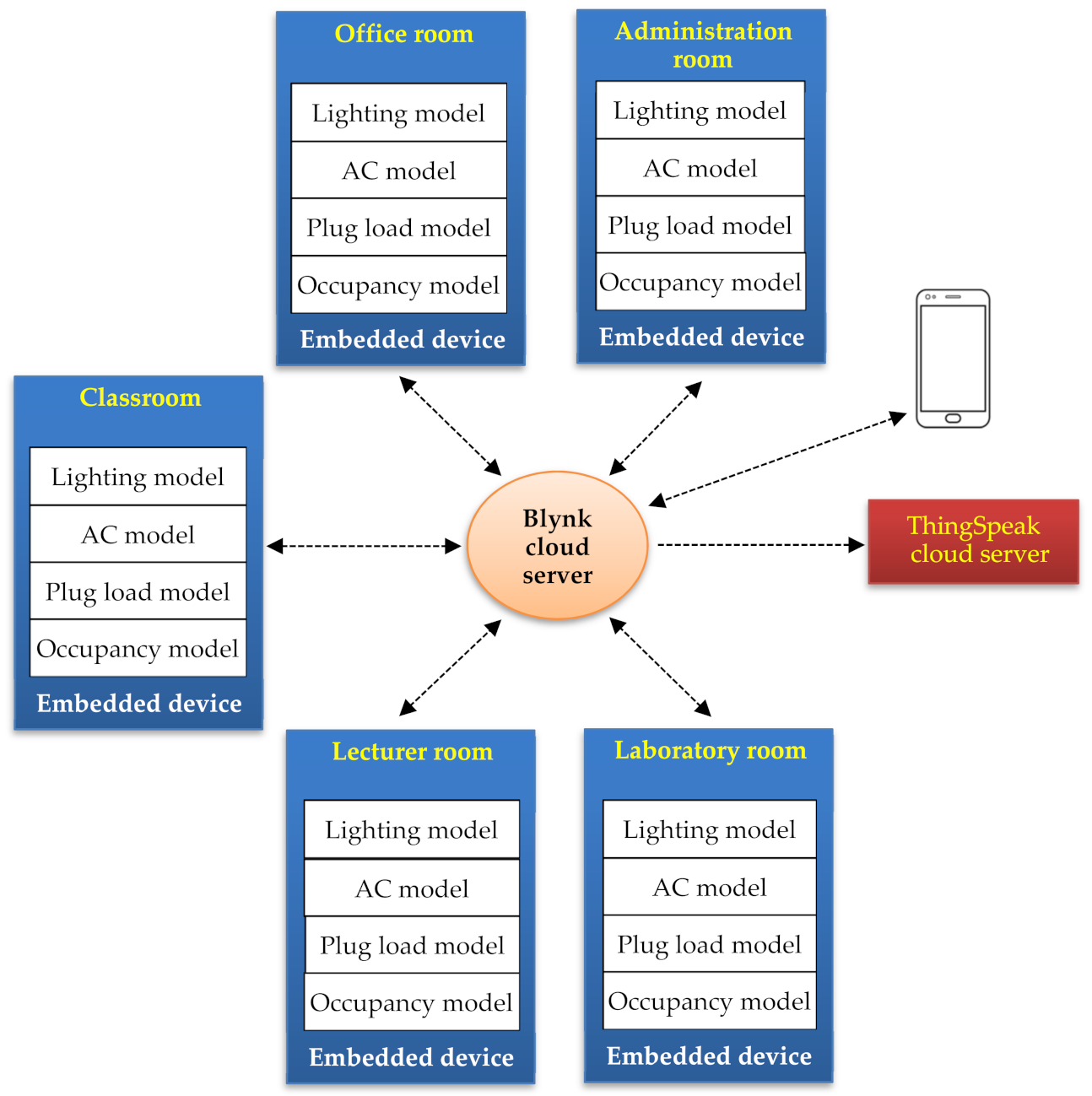
2.2. Architecture

The architecture of the proposed system is illustrated in Figure 2. In this work, we address occupancy-based energy consumption in the main rooms of a campus building, i.e., Office room, Administration room, Classroom, Lecturer room, and Laboratory room. However, the model can be extended to cope with the other rooms in the building. As shown in the figure, each room contained lighting, AC, plug load, and occupancy models. The models were implemented on an Arduino Nano 33 IoT [25], an embedded device equipped with a Wi-Fi module, easily configured to build an IoT application. It is worthy to note that Wi-Fi communication was widely available in the campus building. Thus, the proposed model can easily be adopted for actual application.
IoT technology was adopted to monitor and configure the models implemented on the embedded devices. The benefits of using the IoT platform are:
  • The model parameter can be configured easily from a smartphone.
  • The model can be monitored remotely through the internet.
  • The data generated during the model simulation can easily be stored in the IoT cloud server for further analysis.
  • The developed IoT-based energy monitoring system is applicable for real-time implementation.
Two IoT platforms were employed: Blynk [26] and ThingSpeak [27]. Blynk was employed due to the easy development of the smartphone application. Thus, it was used for setting and configuring the models and as an instant monitoring application, while ThingSpeak was used for long-term data monitoring and storage. As shown in Figure 2, the models were connected to the Blynk cloud server, and then Blynk sent the data to ThingSpeak. The detailed configuration of the IoT-based monitoring system is described in the next section.

2.3. Occupancy-Based Energy Consumption Model

Figure 3 illustrates the model of occupancy-based energy consumption in the campus building. The model was applied in all the rooms described in Figure 2. It consists of five main components: (a) electrical appliances, (b) room environments, (c) occupancy model, (d) occupant behavior model, and (e) energy consumption measurement. Only three typical electrical appliances in the campus building were considered, i.e., the lighting, AC, and the plug load. The plug load can be used by appliances such as computers, printers, and LCD projectors. The room environments were room temperature, which affects the operation of the AC, and room illumination, which affects the operation of the lighting. The occupancy model was used to model the presence of an occupant in the room. Meanwhile, the occupant behavior model was used to model the occupant’s action of switching the electrical appliances on or off. The energy consumption measurement was used to calculate and monitor the consumed energy in the room.
In the occupancy model, the presence of an occupant in the room was determined by its cumulative distributive function [12]. Since the cumulative distributive function (CDF) is calculated from the probability density function (PDF), the user should provide a PDF for each presence activity in the room. The presence activity included arrival at campus, departure from campus, lunch break, and short-term absence (teaching, lunch breaks, and other absences). The PDF of an activity was defined based on the time, duration, and variations given in Table 2.
The occupancy model for the arrival and departure was determined as follows:
  • Calculate the PDF (normal distribution) using the following formula:
    P D F x = 1 σ 2 π e 1 2 x μ σ 2   ,
    where μ is the mean of arrival time (or departure time); σ is the standard deviation, i.e., the time variation of arrival time (or departure time).
  • 2.
    Calculate the CDF using the following formula:
    C D F x = i = 0 x P D F i   ,
    3.
    Generate a random number (RND) between 0 and 1.
    4.
    Find the time k, where CDF(k) = RND.
    5.
    The time k is defined as the time when the occupant is present (absent) in the room.
    The occupant model for teaching, lunch, and other absence was determined similarly, where the above procedure was applied for both the time and duration. The lunchtime and absence time obtained by the previous method determined the start time of the occupant’s absence from the room (all the rooms). The teaching time determined the start time of the occupant’s absence from the Office room and the Lecture room, while it determined the start time of the occupant’s presence in the Classroom and Laboratory room.
    Once the occupant’s status in the room was determined, the occupant’s behavior was modeled. We examined two models of occupant behaviors, namely Model-A and Model-B, as described in the following:

    2.3.1. Model-A

    Model-A is a simple model, where the occupant control is based on the occupant status in the room, as follows:
    • When the occupant is present in the room, the light is switched on; otherwise, it is switched off.
    • When the occupant is present in the room, the AC is switched on; otherwise, it is switched off.
    • When the occupant is present in the room, the plug load power is 100%; otherwise, the plug load power is 0%.

    2.3.2. Model-B

    The occupant control in Model-B is based on the room conditions and the probability of switching the appliances on or off, as proposed in [7,11,14]. The model is described as follows:
    • When the occupant is present, and the room illumination is lower than a threshold, the light is switched on according to the following probability function:
      P L o n = 1 e Δ τ u 1 x L 1 k 1 ,   x u 1 0 ,     x > u 1 ,
      where u1 is the threshold for illumination to switch on the light, L1 is the scale of the function, k1 is the slope of the function, x is the room illumination, and Δτ is time interval.
    • When the occupant is present, and the room illumination is greater than a threshold, the light is switched off according to the following probability function:
      P L o f f = 1 e Δ τ x u 2 L 2 k 2 ,   x u 2 0 ,   x < u 2 ,
      where u2 is the threshold to switch off the light, L2 is the scale of the function, k2 is the slope of the function, x is the room illumination, and Δτ is time interval.
    • When there is no occupant, the light is switched off.
    • When the occupant is present, and the room temperature is greater than a threshold, the AC is switched on according to the following probability function:
      P A C o n = 1 e Δ τ T u 3 L 3 k 3 ,   T u 3 0 ,   T < u 3 ,
      where u3 is the threshold for the temperature to switch on the AC, L3 is the scale of the function, k3 is the slope of the function, T is the room temperature, and Δτ is time interval.
    • When the occupant is present, and the room temperature is lower than a threshold, the AC is switched off according to the following probability function:
      P A C o f f = 1 e Δ τ u 4 T L 4 k 4 ,   T u 4 0 ,     T > u 4 ,
      where u4 is the threshold for the temperature to switch off the AC, L4 is the scale of the function, k4 is the slope of the function, T is the room temperature, and Δτ is time interval.
    • When there is no occupant, the AC is switched off.
    • When the occupant is present in the room, the plug load power is 100%; otherwise, the plug load power is 30% [7].

    2.4. IoT-Based Monitoring System

    2.4.1. IoT System Configuration

    As described previously, we integrated two IoT platforms—Blynk and ThingSpeak—for different purposes. Blynk was used to configure and monitor the models from a smartphone. ThingSpeak was used for data collection and storage. The data communication between an embedded device, Blynk, and ThingSpeak is illustrated in Figure 4. The data were sent from Blynk to the Arduino Nano 33 IoT in the configuration mode using the Blynk protocol. Whereas, in the monitoring mode, the data were sent from the Arduino Nano 33 Iot to Blynk using the Blynk protocol. Then, Blynk forwarded the data to ThingSpeak using a Webhook API (Application Programming Interface).
    The configuration of the whole IoT-based monitoring system is illustrated in Figure 5. ThingSpeak retrieves and stores the data in a channel. One channel consists of eight fields, where each field holds one variable. In this work, one channel was used to monitor and store the occupancy status and each appliance’s power and energy. Since there were three appliances in one room, three channels were required, as shown in Figure 5. Thus, fifteen channels were needed for the proposed system.
    The data in each channel were updated by Blynk using the Webhook widget. Since the widget can only make one request per second, 15 Webhook widgets were needed for a real-time monitoring system. Each Webhook widget is triggered by an embedded device that sends the corresponding data to the Webhook (or ThingSpeak channel). However, it should separate an occupancy model of each room into several devices. To handle such a problem, we utilized the bridge widget of Blynk. The bridge widget provides device-to-device communication through the Blynk server. Using this widget, we exchanged the data between the devices easily. Therefore, as shown in Figure 5, the Arduino Nano 33 IoT modules were configured as the main and bridge devices. The main device was used to perform an occupancy-based energy consumption modeling of a room. A bridge device sends parts of the data to the Webhook for data forwarding to ThingSpeak. There were five main devices, one device for each room, and ten bridge devices were required to send all the monitored data to ThingSpeak. The arrangement of the monitored data of the Office room model is given in Table 3. The other rooms were arranged similarly.
    Referring to Table 3, the Arduino Nano 33 IoT and the main project of the Blynk application (Office room) stored the configuration data and all the monitored data of the Office room model. However, only the occupancy data and the data related to the lighting were sent to the ThingSpeak channel: Office (Lighting). The data related to the AC and plug load were shared with the bridge devices, Office room (AC) and Office room (Plug), and then sent to the respective channel in ThingSpeak.

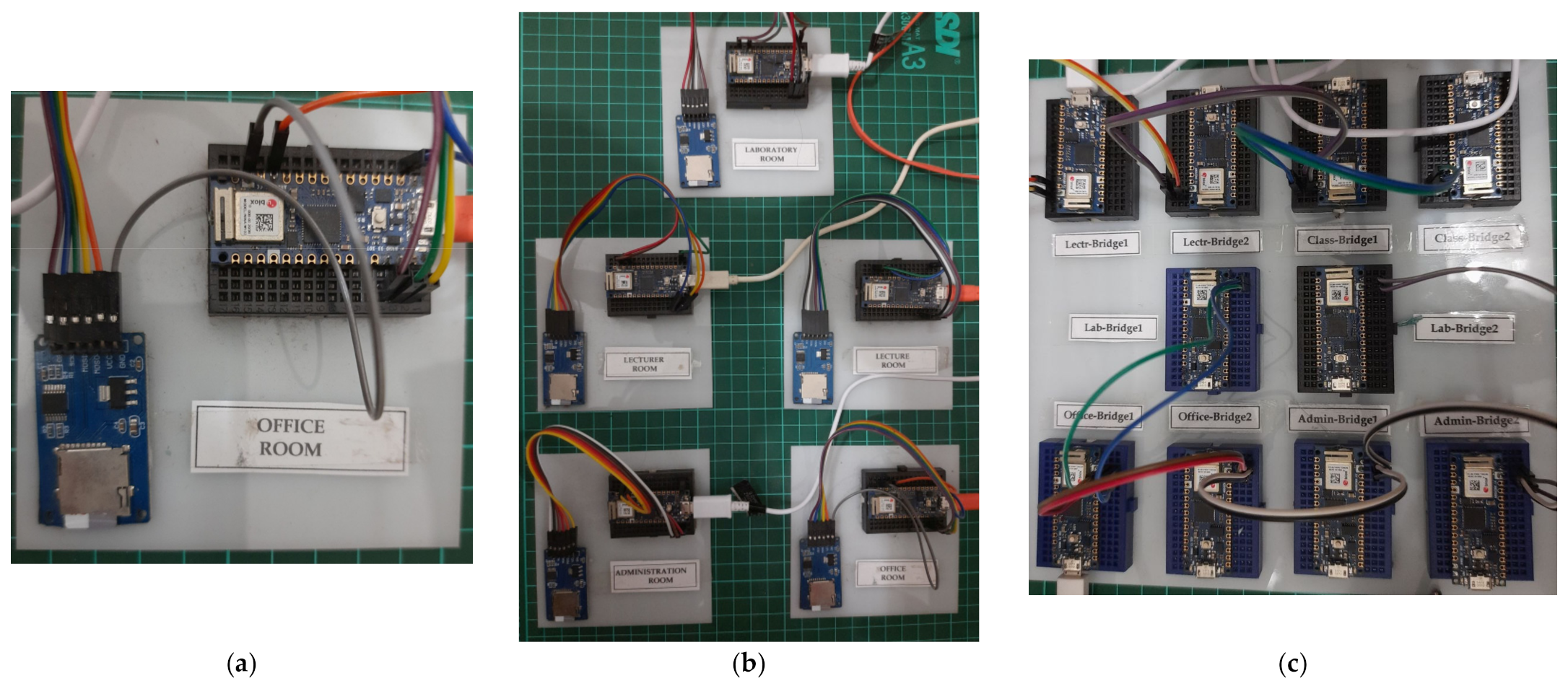
    2.4.2. Hardware Implementation

    The models were implemented on the Arduino Nano 33 IoT, a small embedded system equipped with a Wi-Fi module. The Arduino Nano 33 IoT is based on an SAMD21 Cortex®-M0+ 32bit low-power ARM MCU with a clock speed of 48 MHz, a CPU Flash Memory of 256 KB, and an SRAM of 32 KB. The Wi-Fi module supports 802.11b/g/n in the 2.4 GHz ISM band.
    As described previously, the Arduino Nano 33 IoT is categorized into the main device and bridge device. As shown in Figure 5, the main devices and bridge devices were connected to the internet using the different access points (internet gateway). This arrangement was based on the observation that connecting all 15 devices to the same access point caused network overflow due to the frequently high traffic sent from the devices. The photographs of the hardware prototypes are depicted in Figure 6. Figure 6a shows the main device consisting of an Arduino Nano 33 IoT and an SDCard module. The SDCard was used to save the configuration data and as a storage device for data logging during the experiments. The main and bridge devices groups are shown in Figure 6b,c, respectively.

    3. Experimental Results

    3.1. Configuration of the Model

    For the experiments, the configuration data of each room are given in Table 4. The data were configured and can be changed using the Blynk application. Once the data were sent to the main device, they were saved to the SDCard. The configuration data consisted of the model parameters, the room temperature and illumination, and the simulation setting. Since the teaching time was scheduled weekly, the teaching time data were provided from Monday to Friday. In this work, we assumed that the campus building was utilized during office hours; thus, room temperature and illumination data were provided from 06:00 to 17:00.
    The Blynk application for configuring the Administration room model is depicted in Figure 7. The application for the other rooms was similar. Since the application is run on a smartphone connected to the internet, it is worthy to note that the model can be configured remotely and efficiently. Thus, it provides an efficient way for simulating the model. Further, we can extend it to a real-time simulation system. In this case, the model was implemented on the embedded hardware, which acted as the server; then, users can configure and simulate the model remotely via the internet.
    The simulation setting shown in Figure 7 was used to set the simulation start time and the time interval. The simulation start time defined the time when all embedded devices started to run the model. Since the date and time of each device were synchronized by the Blynk cloud server, it enabled all models to run synchronously. The time interval represents real-time sampling for the data collection and processing of the energy consumption. A time interval of 20 min means that the occupancy data and energy consumption were calculated every 20 min.

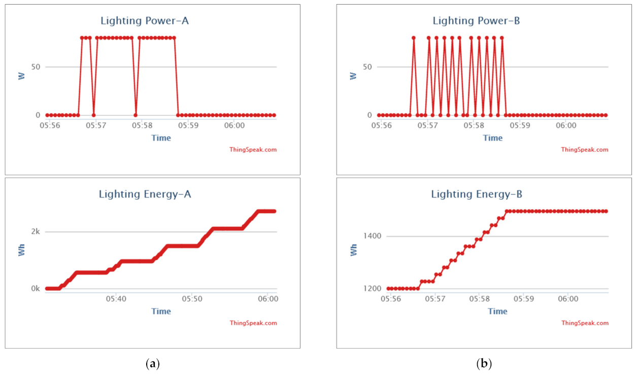
    3.2. Blynk and ThingSpeak Applications

    Besides configuring the model, the Blynk application was also developed to monitor the models implemented on the embedded devices. It monitors the occupancy status, the power, and energy consumed by the appliances. At the top of the application display, the current date and time information, the simulation step, and the simulation day and time are displayed. This helps users to monitor and examine the models in real time.
    Figure 8 shows the monitoring display of the Lecturer room, where the pictures on the left and right sides are the monitoring displays of the lighting and AC, respectively. As shown in the figure, both Model-A and Model-B are displayed. Several GUI widgets such as the status bar, LED indicators, and gauges were used to display the status and values of the monitoring variables. The bright colors of the widgets shown in the right picture indicate the ON status (or occupied), while the dark colors in the left are the OFF status (or unoccupied). The status bar and LED represent the occupant’s status and the appliance (lighting or AC) in the room, respectively. Meanwhile, the gauges display the power consumption. The energy consumptions are shown as the numeric displays.
    Figure 9 shows the Web display of the ThingSpeak IoT platform, where the monitored variables of the energy consumption in the Office room are displayed in line charts. Figure 9a,b show the line charts of the lighting power and energy of Model-A and Model-B, respectively. The time displayed in the figure is the timestamp of the data logging (real-time) by ThingSpeak. As shown in the figure, the patterns of lighting power and energy in Model-A differed from those in Model-B due to the different methods described previously. A detailed evaluation of the models is discussed in the next section.

    3.3. Evaluation of Occupancy-Based Energy Consumption Model

    3.3.1. Evaluation of Occupancy Model

    To evaluate the occupancy model, we simulated the models during five days (Monday to Friday) using the data and parameters given in Table 4. Since the occupancy was calculated using a random number, the results were different for each simulation. Therefore, we ran the simulation twice for the evaluation. The simulation results of the occupancies are illustrated in Figure 10, where the first simulation results are called Trial-1, indicated with the solid lines. The second simulation is called Trial-2, displayed with the dashed lines. Figure 10a–e show the occupancy of the Office room, Administration room, Lecturer room, Classroom, and Laboratory room, respectively.
    Figure 10 shows that the two simulations (trials) occupancies in each room were different, as predicted. However, the arrival time, absence time, teaching time, lunchtime, and departure time followed the ranges given in Table 4. Observing Figure 10d, the number of occupied slot times in a day conformed to teaching sessions on the corresponding day; for instance, there were two occupied slot times on Friday (rightmost line chart in Figure 10d that represent two class sessions. Figure 10e shows that there was no occupancy on Tuesday and Friday in the Laboratory room, which confirms the Laboratory usage given in Table 4.
    To examine the effect of time intervals on the occupancy model, we examined the model using different time intervals: 5 min, 10 min, 15 min, and 20 min. The occupied time during five days of Trial-1, Trial-2, and their variations are listed in Table 5. As shown in the table, several findings were obtained:
    • The variation in time intervals did not significantly affect the occupied time generated by the model in the sense that increasing/decreasing occupied time was not dependent on the interval. The variation of occupied time was more affected by the simulation trials.
    • The maximum variation in the occupied time between Trial-1 and Trial-2 was 360 min, which was obtained in the Office room. Recalling the configuration data in Table 4, the total variations in the arrival time, departure time, lunch duration, and the teaching duration were 450 min (during five days). This result shows that the developed model appropriately generated the occupancy according to the given configuration data.

    3.3.2. Evaluation of Occupant Behavior

    To evaluate the occupant behavior model, we examined the energy consumption of Model-A and Model-B. We explored the effects of the simulation trials, the variation of the time intervals, and the comparison of Model-A and Model-B. To provide a clear explanation, we only examined the Office room and Classroom without loss of generality. Due to a similar characteristic, the Office room, Administration room, and Lecturer room were represented by the Office room, while the Classroom represented the Laboratory and Classroom.
    The simulation results of energy consumptions in the Office room and Classroom for the different simulation trials and time intervals are depicted in Figure 11 and Figure 12, respectively. In the figures, the blue, red, and green denote the energy of Trial-1, Trial-2, and their average. The simulation results of Model-A are shown on the left side, while the results of Model-B are on the right side. The simulation results are displayed in each model for 5, 10, 15, and 20 min time intervals.
    To evaluate the effect of the time interval on the calculation of the energy consumption, we examined the average values of Trial-1 and Trial-2 (green bars in Figure 11 and Figure 12). Since the operation of the appliances in Model-A was directly related to the occupancy status, the average occupied times given in Table 5 were considered in the evaluation. The evaluation results are as follows:
    • The left sides of Figure 11 show that the average energies of the appliances in the Office room increased slightly when the time interval increased from 5 min to 20 min. This was caused by the Office room’s occupied time only changing slightly when the time interval increased, as given in Table 5.
    • Similar to the first result, the average energies in the Classroom of Model-A, shown on the left sides of Figure 12, decreased slightly when the time interval increased. This followed the decrement of the average occupied time of the Classroom given in Table 5.
    To evaluate the effect of the time interval on the calculation of the energy consumption in Model-B, we examined the probability functions of switching the appliances on or off, as described in Section 2.3.2. The evaluation results are as follows:
    • The right sides of Figure 11a and Figure 12a show that the average energies of the lighting increased slightly when the time intervals increased. It can be analyzed from the given data that the probability of switching on the lighting was slightly higher than the probability of switching it off, and the increment in time interval increased the probability. For instance, the PLon and PLoff in 5 min were 0.55 and 0.54, respectively, while the PLon and PLoff in 20 min were 0.8 and 0.79, respectively.
    • The right sides of Figure 11b and Figure 12b show that the average energies of the AC decreased significantly when the time intervals increased. It can be analyzed the given data that the probability of switching on the AC was higher than the probability of switching it off, and the increment in time interval increased the probability. For instance, the PACon and PACoff in 5 min were 0.1 and 0.99, respectively, while the PACon and PACoff in 20 min were 0.33 and 1, respectively.
    • The right sides of Figure 11c and Figure 12c show that the profiles of the average energies of the plug load followed those on the left sides. This was caused by the similar algorithm used in Model-A and Model-B for controlling the plug load. They differed only in the consumed power during the unoccupied time. Therefore, the consumed energy was not affected by the time interval.
    To evaluate the behavior of the Model-A and Model-B in more detail, we compared the profile of energy consumption as illustrated in Figure 13 for the Office room and Figure 14 for the Classroom. In the figures, the blue line represents Model-A1 (Model-A in the first trial), the red line represents Model-B1 (Model-B in the first trial), the green line represents Model-A2 (Model-A in the second trial), the black line represents Model-B2 (Model-B in the second trial). Both models use a time interval of 5 min.
    Figure 13 and Figure 14 show clearly that each model’s profile is almost the same between the first and second trials. It proved that the random number generated by the simulator does not affect the result of the model. It is worthy that the profiles of Model-A do not intersect with Model-B. Thus, we may distinguish Model-A and Model-B easily as described in the following:
    Figure 13a,b and Figure 14a,b show that the energy consumption of the lighting and AC of Model-A was higher than that of Model-B. This result complies with the algorithms of models described in Section 2.3.1 and Section 2.3.2 and show that the energy consumption of the lighting and AC of Model In Model-A, the light and AC will be switched on when the occupant is present. It is regardless of the willingness of the occupant and the room conditions. On the contrary, in Model-B, the light and AC will be switched on based on the room conditions and the occupant’s behavior. Therefore, the energy consumption in Model-A will be higher than Model-B. Model-B is a more realistic model that represents the actual situation, even though, in some conditions, Model-A may be fitted. Observing the results suggests that the automatic control of the light and AC systems based on the occupancy and room conditions may reduce the energy consumption of the building significantly.
    Meanwhile, Figure 13c and Figure 14c show that the energy consumption of the plug load of Model-A was lower than that of Model-B. This result was caused by the fact that, when there was no occupant, the plug load power was 0% and 30% in Model-A and Model-B, respectively. Both models may fit the actual conditions, where Model-A is suitable for a standard building with a few electrical appliances. At the same time, Model-B is ideal for a modern building with complex electrical appliances.

    3.3.3. Evaluation of IoT Data Transmission

    We examined the transmission delay (latency), delay variation (jitter), packer inter-arrival time, and packet loss to evaluate the IoT data transmission. The objective was to assess the reliability of the proposed IoT system for real-time modeling and simulation. In the experiment, one simulation step was 5 s; thus, the data were transmitted from the embedded device every 5 s. The measurement result of the data transmission parameters is given in Table 6. Since the AC and plug load data were transmitted differently from the lighting data, as illustrated in Figure 5 and Figure 6, they were examined separately.
    Referring to Table 6, the evaluation results of each parameter are as follows:
    • The transmission delay (latency) was the delay time between the data transmitted by the embedded device (main device) and the data received by ThingSpeak. The lighting data achieved the fastest latency, i.e., 6.053 s. This conforms to Figure 5 and Figure 6, where the lighting data were transmitted directly from the embedded device to Blynk and then ThingSpeak. Meanwhile, the AC data and plug load data were transmitted via the bridge’s devices. However, it is interesting to note that, even though we used the bridge devices, the latency of the AC data was only slightly higher than the lighting data. This concludes that the highest latency in the plug load data was caused by the internet networks, not the bridge’s architecture.
    • The lighting and plug load data achieved the lowest and highest delay variations (jitter), respectively. This result was caused by a similar condition in the latency discussed above.
    • The packet inter-arrival times of the lighting, AC, and plug load data were almost the same, i.e., about 5 s. Since the data were sent from the embedded devices every 5 s, the result shows that the latency and jitter affected the deviations.
    • Similar to the latency and jitter, the lowest and highest packet losses were achieved by the lighting and plug load data, respectively.
    From the above discussions, we may conclude that our proposed IoT system is suitable for real-time simulations, which accept a minimal time interval between packets of 5 s and a maximum latency of 10 s. This requirement is enough to simulate occupancy-based energy consumption as proposed in this paper. It is worthy to note that, since the proposed real-time simulation employed state-of-the-art IoT platforms, we were able to extend the system for real-time implementation.

    4. Conclusions

    We developed the implementation of occupancy-based energy consumption in a campus building on embedded devices. We integrated modeling and real-time monitoring applications by employing IoT platforms such as the Blynk application for configuration and instant monitoring and ThingSpeak for data logging and long-term monitoring. We evaluated the proposed real-time simulator using two occupant’s behaviors models. The experimental results showed that the models considering the room conditions and the occupant’s behaviors to control the light and AC produce a lower energy consumption than the models based on the occupancy only. We assessed the validity of the implemented model on embedded devices by evaluating several parameters, such as simulation trials and time intervals. The results proved that the implemented model was valid. We also examined the reliability of the proposed real-time modeling simulation by measuring the IoT data transmission parameters such as latency, jitter, inter-arrival time, and packet loss. The results also showed that the proposed approach was reliable for such real-time modeling.
    In the future, the approach will be improved and extended to cope with complex models and buildings. Furthermore, we will investigate integration with the other IoT platforms.

    Author Contributions

    Conceptualization, A.S.; methodology, A.S.; software, A.S. and S.S.; validation, A.S. and S.S.; data curation, A.S. and S.S.; writing—original draft preparation, A.S.; writing—review and editing, A.S. and S.S. All authors have read and agreed to the published version of the manuscript.

    Funding

    This work was supported by a Research Grant from the Ministry of Education, Culture, Research, and Technology, Republic of Indonesia, Year 2021 (No.: 167/E4.1/AK.04.PT/2021).

    Conflicts of Interest

    The authors declare no conflict of interest.

    References

    1. Marques, G.; Pitarma, R. Monitoring energy consumption system to improve energy efficiency. Adv. Intell. Syst. Comput. 2017, 570, 3–11. [Google Scholar] [CrossRef]
    2. Paone, A.; Bacher, J.P. The impact of building occupant behavior on energy efficiency and methods to influence it: A review of the state of the art. Energies 2018, 11, 953. [Google Scholar] [CrossRef] [Green Version]
    3. Ding, Y.; Wang, Q.; Wang, Z.; Han, S.; Zhu, N. An occupancy-based model for building electricity consumption prediction: A case study of three campus buildings in Tianjin. Energy Build. 2019, 202. [Google Scholar] [CrossRef]
    4. Delzendeh, E.; Wu, S.; Lee, A.; Zhou, Y. The impact of occupants’ behaviours on building energy analysis: A research review. Renew. Sustain. Energy Rev. 2017, 80, 1061–1071. [Google Scholar] [CrossRef]
    5. Zhu, P.; Gilbride, M.; Yan, D.; Sun, H.; Meek, C. Lighting energy consumption in ultra-low energy buildings: Using a simulation and measurement methodology to model occupant behavior and lighting controls. Build. Simul. 2017, 10, 799–810. [Google Scholar] [CrossRef]
    6. Song, L.; Zhou, X.; Zhang, J.; Zheng, S.; Yan, S. Air-Conditioning usage pattern and energy consumption for residential space heating in Shanghai China. Procedia Eng. 2017, 205, 3138–3145. [Google Scholar] [CrossRef]
    7. Sun, K.; Hong, T. A simulation approach to estimate energy savings potential of occupant behavior measures. Energy Build. 2017, 136, 43–62. [Google Scholar] [CrossRef] [Green Version]
    8. Chen, Y.; Liang, X.; Hong, T.; Luo, X. Simulation and visualization of energy-related occupant behavior in office buildings. Build. Simul. 2017, 10, 785–798. [Google Scholar] [CrossRef]
    9. Yan, D.; Xia, J.; Tang, W.; Song, F.; Zhang, X.; Jiang, Y. DeST—An integrated building simulation toolkit part I: Fundamentals. Build. Simul. 2008, 1, 95–110. [Google Scholar] [CrossRef]
    10. Zhou, X.; Yan, D.; Hong, T.; Ren, X. Data Analysis and stochastic modeling of lighting energy use in large office buildings in China. Energy Build. 2015, 86, 275–287. [Google Scholar] [CrossRef] [Green Version]
    11. Wang, C.; Yan, D.; Ren, X. Modeling individual’s light switching behavior to understand lighting energy use of office building. Energy Procedia 2016, 88, 781–787. [Google Scholar] [CrossRef] [Green Version]
    12. Chen, Y.; Hong, T.; Luo, X. An agent-based stochastic occupancy simulator. Build. Simul. 2018, 11, 37–49. [Google Scholar] [CrossRef] [Green Version]
    13. Occupancy Simulator. Available online: http://occupancysimulator.lbl.gov/ (accessed on 21 June 2021).
    14. Ren, X.; Yan, D.; Wang, C. Air-Conditioning Usage Conditional Probability Model for Residential Buildings. Build. Environ. 2014, 81, 172–182. [Google Scholar] [CrossRef]
    15. EnergyPlus. Available online: https://energyplus.net/ (accessed on 15 September 2021).
    16. Hong, T.; Sun, H.; Chen, Y.; Taylor-Lange, S.C.; Yan, D. An occupant behavior modeling tool for co-simulation. Energy Build. 2016, 117, 272–281. [Google Scholar] [CrossRef] [Green Version]
    17. Occupant Behavior Research at LBNL BTUS. Available online: https://behavior.lbl.gov/?q=node/4 (accessed on 21 June 2021).
    18. Anylogic. Available online: https://www.anylogic.com/ (accessed on 21 June 2021).
    19. Zhao, L.; Zhang, J.L.; Liang, R.B. Development of an energy monitoring system for large public buildings. Energy Build. 2013, 66, 41–48. [Google Scholar] [CrossRef]
    20. Liu, Y.; Leng, J.; Sun, B. Design of a energy monitoring system based on WebAccess. In Proceedings of the 29th Chinese Control Decision. Conference CCDC, Chongqing, China, 28–30 May 2017; pp. 4099–4103. [Google Scholar] [CrossRef]
    21. Sesotya Utami, S.; Faridah Azizi, N.A.; Kencanawati, E.; Tanjung, M.A.; Achmad, B. Energy monitoring system for existing buildings in Indonesia. E3S Web Conf. 2018, 42, 1–7. [Google Scholar] [CrossRef]
    22. Priyadarshini, R.; Reddyb, S.R.N.; Mehra, R.M. Occupancy-based energy management and campus monitoring using wireless sensor network. Int. J. Eng. Technol. 2015, 15, 56. [Google Scholar]
    23. Wei, C.; Li, Y. Design of energy consumption monitoring and energy-saving management system of intelligent building based on the Internet of Things. In Proceedings of the International Conference on Electronics, Communications and Control (ICECC), Ningbo, China, 9–11 September 2011; pp. 3650–3652. [Google Scholar] [CrossRef]
    24. Gomes, L.; Sousa, F.; Vale, Z. An agent-based iot system for intelligent energy monitoring in buildings. In Proceedings of the IEEE Conference on Vehicular Technology (VTC), Porto, Portugal, 3–6 June 2018; pp. 1–5. [Google Scholar] [CrossRef]
    25. Arduino Nano 33 IoT. Available online: https://store.arduino.cc/usa/nano-33-iot (accessed on 30 July 2021).
    26. Blynk. Available online: https://blynk.io/ (accessed on 20 July 2021).
    27. ThingSpeak. Available online: https://thingspeak.com/ (accessed on 20 July 2021).
    Figure 1. Proposed real-time simulation system.
    Figure 1. Proposed real-time simulation system.
    Electronics 10 02307 g001
    Figure 2. Architecture of proposed system.
    Figure 2. Architecture of proposed system.
    Electronics 10 02307 g002
    Figure 3. Block diagram of occupancy-based energy consumption model.
    Figure 3. Block diagram of occupancy-based energy consumption model.
    Electronics 10 02307 g003
    Figure 4. Data communication between embedded device, Blynk, and ThingSpeak.
    Figure 4. Data communication between embedded device, Blynk, and ThingSpeak.
    Electronics 10 02307 g004
    Figure 5. IoT system configuration.
    Figure 5. IoT system configuration.
    Electronics 10 02307 g005
    Figure 6. Photographs of the hardware prototypes: (a) main device; (b) group of main devices; (c) group of bridge devices.
    Figure 6. Photographs of the hardware prototypes: (a) main device; (b) group of main devices; (c) group of bridge devices.
    Electronics 10 02307 g006
    Figure 7. Blynk application for configuring the models.
    Figure 7. Blynk application for configuring the models.
    Electronics 10 02307 g007
    Figure 8. Blynk application for monitoring the models.
    Figure 8. Blynk application for monitoring the models.
    Electronics 10 02307 g008
    Figure 9. Line chart display for ThingSpeak: (a) lighting power and energy of Model-A; (b) lighting power and energy of Model-B.
    Figure 9. Line chart display for ThingSpeak: (a) lighting power and energy of Model-A; (b) lighting power and energy of Model-B.
    Electronics 10 02307 g009
    Figure 10. Simulation results of the occupancy model: (a) Office room; (b) Administration room; (c) Lecturer room; (d) Classroom; (e) Laboratory room.
    Figure 10. Simulation results of the occupancy model: (a) Office room; (b) Administration room; (c) Lecturer room; (d) Classroom; (e) Laboratory room.
    Electronics 10 02307 g010
    Figure 11. Energy consumption in the Office room: (a) lighting energy; (b) AC energy; (c) plug load energy.
    Figure 11. Energy consumption in the Office room: (a) lighting energy; (b) AC energy; (c) plug load energy.
    Electronics 10 02307 g011
    Figure 12. Energy consumption in the Classroom: (a) lighting energy; (b) AC energy; (c) plug load energy.
    Figure 12. Energy consumption in the Classroom: (a) lighting energy; (b) AC energy; (c) plug load energy.
    Electronics 10 02307 g012
    Figure 13. Profile of energy consumption in the Office room: (a) lighting energy; (b) AC energy; (c) plug load energy.
    Figure 13. Profile of energy consumption in the Office room: (a) lighting energy; (b) AC energy; (c) plug load energy.
    Electronics 10 02307 g013aElectronics 10 02307 g013b
    Figure 14. Profile of energy consumption in the Classroom: (a) lighting energy; (b) AC energy; (c) plug load energy.
    Figure 14. Profile of energy consumption in the Classroom: (a) lighting energy; (b) AC energy; (c) plug load energy.
    Electronics 10 02307 g014aElectronics 10 02307 g014b
    Table 1. Comparison between existing and proposed systems.
    Table 1. Comparison between existing and proposed systems.
    Ref.Software SimulationReal-Time System
    ModelDashboard Monitoring SystemHardware Platform
    OccupancyOccupant BehaviorEnergy ConsumptionWeb
    Application
    Mobile
    Application
    Desktop
    Application
    Sensor
    Systems
    Communication Protocol
    DesT [9]
    Occupancy Simulator [13]
    EnergyPlus [15]
    obFMU [17]
    [8]
    [1] SmartPlugWi-Fi
    [19] Energy metersRS-485
    [22] Smart sensorsZigbee
    [24] SmartPlugWi-Fi
    Proposed Embedded simulatorWi-Fi
    Table 2. Data input of the presence activity.
    Table 2. Data input of the presence activity.
    ActivityData InputRoom
    ArrivalTime of arrival, time variationOffice room, Administration room, Lecturer room
    DepartureTime of departure, time variationOffice room, Administration room, Lecturer room
    TeachingTeaching time, time variation, duration, duration variationOffice room, Lecturer room, Classroom, Laboratory room
    Lunch breakLunchtime, time variation, duration, duration variationOffice room, Administration room, Lecturer room
    Other leavingAbsence time, time variation, duration, duration variationOffice room, Administration room, Lecturer room
    Table 3. Arrangement of monitored data of the Office room model.
    Table 3. Arrangement of monitored data of the Office room model.
    Arduino Nano 33 IoT
    (Main Device)
    Arduino Nano 33 IoT
    (Bridge Device)
    BlynkThingSpeak
    #1: Office room Project name: Office room (Main)Channel name: Office (Lighting)
    -Configuration
    -Lighting Monitoring
    Lighting Power—Model-AField-1: Lighting Power—Model-A
    Lighting Energy—Model-AField-2: Lighting Energy—Model-A
    Lighting Power—Model-BField-3: Lighting Power—Model-B
    Lighting Energy—Model-BField-4 Lighting Energy—Model-B
    -AC Monitoring
    -Plug load Monitoring
    #6: Office Room (AC)Project name: Office—AC (Bridge)Channel name: Office (AC)
    AC Power—Model-AField-1: AC Power—Model-A
    AC Energy—Model-AField-2: AC Energy—Model-A
    AC Power—Model-BField-3: AC Power—Model-B
    AC Energy—Model-BField-4 AC Energy—Model-B
    #7: Office Room (Plug)Project name: Office—Plug (Bridge)Channel name: Office (AC)
    Plug Power—Model-AField-1: Plug Power—Model-A
    Plug Energy—Model-AField-2: Plug Energy—Model-A
    Plug Power—Model-BField-3: Plug Power—Model-B
    Plug Energy—Model-BField-4 Plug Energy—Model-B
    Table 4. Data and parameters of the models.
    Table 4. Data and parameters of the models.
    Data/ParameterOffice RoomAdministration RoomLecturer RoomClassroomLaboratory Room
    Arrival time; variation (min)08:00; 3008:00; 3008:00; 30NANA
    Departure time; variation (min)16:00; 3016:00; 3016:00; 30NANA
    Lunchtime; variation (min);
    Lunch duration; variation (min)
    12:00; 30; 60; 1512:00; 30; 60; 1512:00; 30; 60; 15NANA
    Teaching time; variation (min); Teaching duration; variation (min)Monday00:00; 00; 000; 00NA10:00; 10; 100; 3008:00; 20; 100; 30;
    10:00; 20; 100; 30;
    13:00; 20; 150; 30
    08:00; 20; 180; 30; 13:00; 20; 180; 30; 10:00; 00; 000; 00
    Tuesday09:00; 20; 150; 30NA00; 00; 00; 000; 0009:00; 20; 150; 30;
    13:00; 20; 150; 30;
    00:00; 00; 000; 00
    00:00; 00; 000; 00; 00:00; 00; 000; 00; 00:00; 00; 000; 00
    Wednesday00:00; 00; 000; 00NA09:00; 10; 100; 3008:00; 20; 100; 30;
    10:00; 20; 150; 30;
    14:00; 20; 100; 30
    08:00; 20; 180; 30; 13:00; 20; 180; 30; 10:00; 00; 000; 00
    Thursday00:00; 00; 000; 00NA13:00; 10; 150; 3008:00; 20; 100; 30; 10:00; 20; 100; 30; 14:00; 20; 100; 3008:00; 20; 180; 30; 13:00; 20; 180; 30; 10:00; 00; 000; 00
    Friday00:00; 00; 000; 00NA00:00; 00; 000; 0008:00; 20; 100; 30; 14:00; 20; 100; 30; 00:00; 00; 000; 0000:00; 00; 000; 00; 00:00; 00; 000; 00; 00:00; 00; 000; 00
    Leaving time; variation (min);
    Teaching duration; variation (min); probability (%)
    09:00; 30; 090; 30; 4009:00; 30; 060; 30; 1009:00; 30; 090; 30; 20NANA
    Room temperature (°C); Room illumination (lux)Time: 6 h25.00; 000.0025.00; 000.0025.00; 000.0025.00; 000.0025.00; 000.00
    Time: 7 h25.00; 000.0025.00; 000.0025.00; 000.0025.00; 000.0025.00; 000.00
    Time: 8 h25.50; 000.0025.50; 000.0025.50; 000.0025.50; 050.0025.50; 000.00
    Time: 9 h28.00; 000.0028.00; 000.0028.00; 000.0028.00; 100.0028.00; 000.00
    Time: 10 h28.00; 000.0028.00; 000.0028.00; 000.0028.00; 100.0028.00; 000.00
    Time: 11 h29.00; 000.0029.00; 000.0029.00; 000.0029.00; 100.0029.00; 000.00
    Time: 12 h29.00; 000.0029.00; 000.0029.00; 000.0029.00; 100.0029.00; 000.00
    Time: 13 h30.00; 000.0030.00; 000.0030.00; 000.0030.00; 100.0030.00; 000.00
    Time: 14 h28.00; 000.0028.00; 000.0028.00; 000.0028.00; 100.0028.00; 000.00
    Time: 15 h27.00; 000.0027.00; 000.0027.00; 000.0027.00; 050.0027.00; 050.00
    Time: 16 h25.00; 000.0025.00; 000.0025.00; 000.0025.00; 050.0025.00; 050.00
    Time: 17 h24.00; 000.0024.00; 000.0024.00; 000.0024.00; 000.0024.00; 000.00
    Parameters for AC control: u3; L3; k3; u4; L4; k427.75; 15.87; 2.22;
    30.25; 152.88; 1.30
    27.75; 15.87; 2.22;
    30.25; 152.88; 1.30
    27.75; 15.87; 2.22;
    30.25; 152.88; 1.30
    27.75; 15.87; 2.22;
    30.25; 152.88; 1.30
    27.75; 15.87; 2.22;
    30.25; 152.88; 1.30
    Parameters for lighting control: u1; L1; k1; u2; L2; k2325.00; 430.00; 09.00; 175.00; 2300.00; 1.3027.75; 15.87; 2.22;
    30.25; 152.88; 1.30
    27.75; 15.87; 2.22;
    30.25; 152.88; 1.30
    27.75; 15.87; 2.22;
    30.25; 152.88; 1.30
    27.75; 15.87; 2.22;
    30.25; 152.88; 1.30
    Simulation start time; time interval (Δτ) (min)18:00; 0518:00; 0518:00; 0518:00; 0518:00; 05
    Table 5. Results of occupancy using different time intervals.
    Table 5. Results of occupancy using different time intervals.
    Occupied Time during 5 Days (Min)
    OfficeAdmin.LecturerClassroomLaboratory
    Time interval =
    5 min
    Trial-116901820166515351075
    Trial-218601805171013251050
    Average17751812.51687.514301062.5
    Variation170154521025
    Time interval =
    10 min
    Trial-11780203018001420880
    Trial-21720197018601520930
    Average1750200018301470905
    Variation60606010050
    Time interval =
    15 min
    Trial-11980210018751140915
    Trial-216201845183013051110
    Average18001972.51852.51222.51012.5
    Variation36025545165195
    Time interval =
    20 min
    Trial-11900182017201260960
    Trial-21820212017601040860
    Average1860197017401150910
    Variation8030040220100
    Table 6. IoT data transmission measurement.
    Table 6. IoT data transmission measurement.
    Lighting DataAC DataPlug Load Data
    Transmission delay (latency)6.0153 s6.4735 s9.0348 s
    Delay variation (jitter)0.2704 s0.6270 s0.9829 s
    Packet inter-arrival time5.1763 s5.4371 s5.5085 s
    Packet loss1.11%5.42%10.8%
    Publisher’s Note: MDPI stays neutral with regard to jurisdictional claims in published maps and institutional affiliations.

    Share and Cite

    MDPI and ACS Style

    Soetedjo, A.; Sotyohadi, S. Modeling of Occupancy-Based Energy Consumption in a Campus Building Using Embedded Devices and IoT Technology. Electronics 2021, 10, 2307. https://doi.org/10.3390/electronics10182307

    AMA Style

    Soetedjo A, Sotyohadi S. Modeling of Occupancy-Based Energy Consumption in a Campus Building Using Embedded Devices and IoT Technology. Electronics. 2021; 10(18):2307. https://doi.org/10.3390/electronics10182307

    Chicago/Turabian Style

    Soetedjo, Aryuanto, and Sotyohadi Sotyohadi. 2021. "Modeling of Occupancy-Based Energy Consumption in a Campus Building Using Embedded Devices and IoT Technology" Electronics 10, no. 18: 2307. https://doi.org/10.3390/electronics10182307

    Note that from the first issue of 2016, this journal uses article numbers instead of page numbers. See further details here.

    Article Metrics

    Back to TopTop