Co-Simulation Analysis for Performance Prediction of Synchronous Reluctance Drives

Abstract

To improve the design of electric drives and to better predict the system performance, numerical simulation has been widely employed. Whereas in the majority of the approaches, the machines and the power electronics are designed and simulated separately, to improve the fidelity, a co-simulation should be performed. This paper presents a complete coupled co-simulation model of synchronous reluctance machine (SynRel) drive, which includes the finite element model of the SynRel, the power electronics inverter, the control system, and application examples. The model of SynRel is based on a finite element model (FEM) using Simcenter MagNet. The power electronics inverter is built using PLECS Blockset, and the drive control model is built in Simulink environment, which allows for coupling between MagNet and PLECS. The proposed simulation model provides high accuracy thanks to the complete FEA-based model fed by actual inverter voltage. The comparison of the simulation results with experimental measurements shows good correspondence.

1. Introduction

The use of dynamic simulation in order to predict the performance of electrical drives is highly important for the design of electromechanical systems. In the simplest approach, the reduced-order models are used for the simulation of electric drives, where the machine is modeled by a set of differential equations and the electromagnetic nature is taken into account by constant coefficients (lumped parameters); for example, the flux-current relation is assumed linear or replaced by a look-up table, and the power electronics inverter is replaced by an ideal sinusoidal voltage source [1,2,3,4]. This approach allows us to obtain sufficient information about the performance of the drive, but it cannot identify and investigate certain transient and harmonic effects caused by the non-sinusoidal flux density distribution, the slotting effects, and the pulse-width modulated (PWM) voltage source inverter, which are necessary for optimization of the drive and result in higher electromagnetic losses and torque ripple [5]. Moreover, it is well known that the behavior of an electrical machine becomes more nonlinear depending on the operation conditions, the effects of magnetic saturation, and cross-saturation, which should be taken into account [6].

A synchronous reluctance machine (SynRel) is a valid alternative to other AC machines and is well suited for different applications [7,8,9]. Since in the SynRel the losses in the rotor are almost null, this machine has a higher efficiency compared with the induction machine, and the manufacturing process is relatively easy, which leads to lower cost. Moreover, thanks to the inherently salient behavior, SynRel is suitable for sensorless application [10,11]. On the other hand, the magnetic saturation and cross-saturation effects as well as high torque ripple have a large impact on the performance of the machine. As a consequence, an accurate model for simulation of SynRel drive is required for an evaluation of the machine’s behavior and a control strategy optimization.

In order to enhance the simulation fidelity, it is essential to use a model of SynRel drive that is as detailed as possible. In this case, a co-simulation can be used, which allows us to integrate the most suitable simulation tool for each part of the model in a multi-domain analysis [12]. The multi-domain simulation model consists of the finite element model (FEM) model of the electric motor, the power electronics inverter, and the control unit [13,14]. The modular structure of the model allows us to replace one sub-model while leaving the rest unchanged; for example, a slow but detailed model can be replaced by a faster but simplified version depending on performance requirement. Carrying out the co-simulation makes it possible to evaluate the overall performances of the system and to analyze some performance problems due to the interaction between the motor and power electronics inverter, and the influence of different control strategies on the system performance. Thus, the design performance can be validated without physical prototyping, decreasing the cost and validation time [15]. Despite of high degree of accuracy, finite element analysis (FEA) is computationally expensive, especially when Pulse Width Modulated (PWM) inverter is involved. The FEA is carried out at each sample time, and this must be sufficiently small to comply with the dynamics of the overall drive system, resulting in a high computation time. In general, there are mainly two approaches to reducing the simulation time [16]. The first approach is to take full advantage of the computational resources of the computer, such as parallel and distributed computation. The time decomposition method (TDM) is another effective option for parallel computation realized by simulating several time steps simultaneously instead of solving a transient problem sequentially [17,18]. However, the implementation of simulation time reduction techniques is outside the scope of this paper.

2. Co-Simulation Structure

A typical electric motor drive system normally consists of five main parts: a power supply (rectified AC voltage source or DC source), the power electronics inverter, the electric motor, a digital controller for executing algorithms to control the motor, and a driven mechanical system, as shown in Figure 1.

According to the typical structure of electric drive, the coupled co-simulation model of the SynRel drive discussed in this work consists of the following components:

• FE-based SynRel model in Simcenter MagNet;
• Power electronics inverter model in PLECS Blockset (as the DC link voltage source, the ideal DC source is used due to the experimental rig configuration);
• Control system with space vector PWM modulator in MATLAB/Simulink.

MATLAB/Simulink is used as the main simulation tool; thus, PLECS Blockset and MagNet are called through S-functions. The control system is implemented in Simulink, provides the PWM switching signals for the inverter, and then feeds the inverter output voltages at the terminals of FE-based SynRel model. The outputs of the machine model give the phase currents, position, speed, and torque, which are used as feedback for the control unit.

Figure 2 shows the structure of the coupled co-simulation model based on field-oriented control (FOC).

In Figure 3, the data flow in the co-simulation structure is shown.

The following subsections give brief descriptions of the components.

2.1. Complete FE-Based SynRel Model

Finite element simulations were run for SynRel using the commercial package Simcenter MagNet with 2D FEA solver.

The rated data for the FE model are shown in

Table 1. SynRel rated data.

Parameter	Value	Parameter	Value
DC link voltage [V]	540	Stator outer diameter [mm]	260
Rated current [Apk]	44.2	Airgap thickness [mm]	0.5
Rated power [kW]	15	Rotor outer diameter [mm]	169
Rated torque [Nm]	95	Stack length [mm]	205

.

The SynRel is a 48 slot, 4 pole motor, and its cross section is shown in Figure 4. Instead of simulating the entire machine, just a quarter (one pole) can be simulated, exploiting the periodic symmetry of the motor to reduce the size of the problem and to decrease the simulation time.

In the case using one pole of the SynRel, the torque and flux values should be scaled as follows

$$T_{em}=T_{sim}\frac{Q}{Q_{sim}},$$

(1)

$${\psi }_s={\psi }_{sim}\frac{Q}{Q_{sim}},$$

(2)

where $Q_{sim}$ and Q are the simulated and total number of slots, $T_{sim}$ and ${\psi }_{sim}$ are computed by the FE-model torque and flux values, and $T_{em}$ and ${\psi }_s$ are total torque and flux of the SynRel.

Both the rotor and stator laminations’ magnetic material is M270-50A iron, and its B–H curve property is presented in Figure 5.

After setting up the FE model of the SynRel, the simulation is performed using the current source operation to evaluate the machine performance. The rotor magnetic pole axis (d-axis) is aligned with the magnetic axis of phase A. A transient 2D magnet is used to analyse the SynRel performers when it is rotating at 1500 rpm and rated current [11]. The flux density map and the flux lines distribution are presented in Figure 6.

The SynRel with rated load working at the knee of the region of the B–H curve. This type of machine presents only reluctance torque. Its torque production depends on the d and q axis inductance difference ($L_d-L_q$), or more commonly the saliency ratio $\xi$, which is affected by saturation and cross-saturation. Therefore, the analysis of the flux behavior of the SynRel is essential.

The flux-current characteristics, also called flux maps, are obtained using FEA by running simulations on a regular grid over the ($i_d$,$i_q$) plane and reported in Figure 7.

FEA allows us to obtain additional data, such as the average electromagnetic torque $T_{em}$($i_d$,$i_q$) and the peak-to-peak torque ripple $T_{p-p}$($i_d$,$i_q$) maps (Figure 8), etc.

To investigate the discrepancy between the FEA and experimental results, the magnetic model of SynRel was identified using the constant-speed method [19]. The identification procedure is based on the current injection throughout the entire dq-current plane (up to rated current) of the SynRel while it is driven at constant speed by an induction machine electric drive (the experimental setup description is given in Section 4). After obtaining the flux, maps they can be compared with the FEA results by the calculation flux error, defined as

$${\tilde{\psi }}_{dq}={\psi }_{dq.c.s}-{\psi }_{dq.FEA},$$

(3)

where ${\psi }_{dq.FEA}$ and ${\psi }_{dq.c.s}$ are the flux obtained by means of FEA and the constant-speed test, respectively.

The comparison between the flux maps is presented in Figure 9.

As can be observed, the maximum flux errors are 0.06 Vs and 0.045 Vs for the d- and q-axes, respectively.

The experimental platform was equipped with a torque meter, allowing for torque measurement during the constant-speed identification. The measured torque map was compared with FEA estimated torque, as shown in Figure 10. The maximum torque estimation error is around 7 Nm (about 7% of rated torque) is acceptable.

A typical problem of the SynRel is the high torque ripple due to the interaction between the space harmonics and the rotor anisotropy [20]. The FE-based co-simulation model allows us to evaluate the torque ripple and to investigate different control strategies aimed at reducing the torque ripple.

The torque ripple has been evaluated at low speed 5 rpm in order to capture the high-frequency nature of the torque oscillations. The test was carried out at $T_m^{*}$= 20 Nm (according to MTPA trajectory $i_d$ = 10 A, $i_q$ = 11.5 A). Figure 11 presents the experimental and FE evaluations of the torque. As can be observed, the torque ripple waveform amplitudes determined via FE match the experimental data very well. In order to validate the harmonic content of the torque ripple, the Fast Fourier transformation is used. As can be seen in Figure 11, the higher torque ripple amplitudes are expected for even harmonics of order 6, 12, 18, 24, 30, and 36 (giving only lower-order harmonics) [21,22].

Based on these results, it can be said that the FE simulations predict the torque ripple accurately, with a slight overestimation and correct harmonics content.

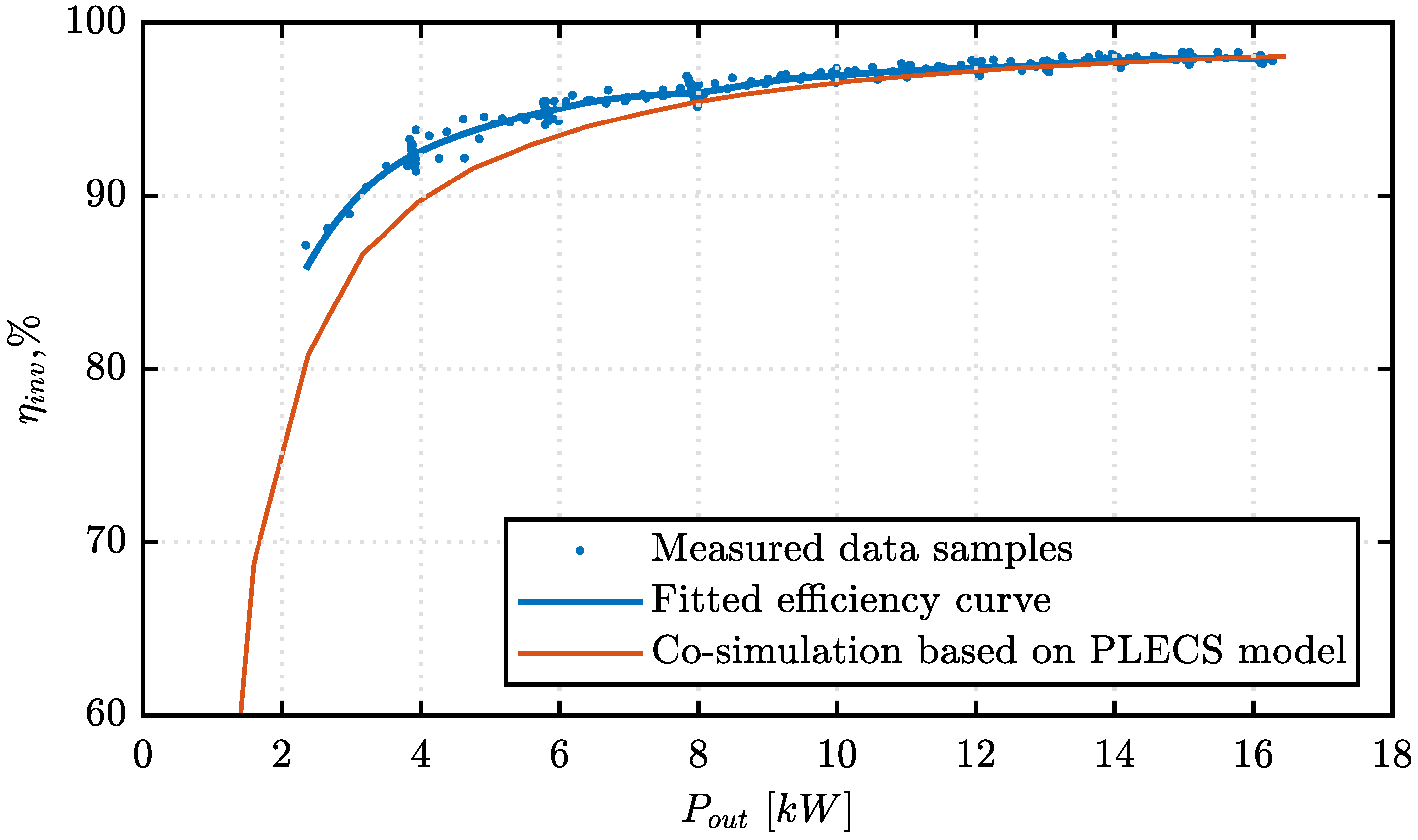
2.2. Power Electronics Inverter Model

Figure 12 shows the implemented PLECS simulation structure of a three-phase inverter. The PWM signals ($S_a$, $S_b$, and $S_c$) are generated from the control scheme in MATLAB using the SVPWM modulator. The current sources simulate the load of the inverter using the currents from FE-based SynRel model. IGBTs and diodes are parameterized according to the datasheet of the power IGBT module.

The inverter of SynRel drive is made of IGBT power modules Semikron SKiM459 GD12E4. The main parameters are collected in

Table 2. SKiM459GD12E4 parameters for the PLECS model.

Parameter	Value
Forward diode voltage [V]	2.14
Diode on-resistance [mOhm]	1.87
Forward IGBT voltage [V]	1.85
IGBT on-resistance [mOhm]	2.3

In order to calculate the efficiency of the inverter, semiconductors losses are estimated using the thermal model of the inverter in PLECS. These semiconductor losses can be classified as conduction and switching losses. The conduction losses can be computed using the on-state voltage as a function of the device current and the device temperature u = $u_{on}(i,T)$. Switching losses occur because the transitions from on-state to off-state and vice versa do not occur instantaneously. During the transition interval, both the current through and the voltage across the device are substantially larger than zero, which leads to large instantaneous power losses. The switching losses are computed by using the fact that, for a given circuit, the current and voltage waveforms during the transition and therefore the total loss energy are principally a function of the pre- and post-switching conditions and the device temperature $E=E_{on}(u_{block},i_{block},T)$, $E=E_{off}(u_{block},i_{block},T)$.

In Figure 13, the model of power electronics inverter is validated by comparing model and measured efficiency curves as a function of output power.

As can be seen from Figure 13, the results above 8 kW show an acceptable match between experiment and simulation with a thermal model.

2.3. Control System Model

Control system includes three types: current, torque, and speed control based on FOC. The FOC block is implemented in Simulink/MATLAB and consists of two internal current loops and one outer speed loop. The speed loop uses a Maximum Torque Per Ampere (MTPA) table to obtain the reference current signals for the internal loops [23]. The MTPA trajectory was obtained by using FEA results. The inputs to this control scheme are the three motor currents $i_a,i_b,i_c$, the motor speed, the position, and the DC link voltage $u_{dc}$, while it outputs PWM signals $S_a,S_b,S_c$ for the power electronic inverter.

In order to validate the complete coupled co-simulation model, co-simulation results were compared with the experimental results. To ensure the comparability of both the results, the simulation was performed with the same current PI controller settings and sampling time of 100 $\mathsf{\mu }\mathrm{s}$. The first test was conducted at standstill (locked rotor) to exclude the influence of the mechanical part of the experimental setup. The response to the $i_d$ = 16 A current step was observed at t = 0.2 s. Then, at t = 0.5 s, the $i_q$ = 22 A step was injected as well to obtain 50 Nm according to MTPA conditions. During this operation, the d-component of the current was kept unchanged at a constant value. In the second test, the SynRel was driven by prime mover, starting at t = 0 s from zero initial value and reaching the value of 500 rpm; at time t = 0.25 s, a constant value of $i_d$ = 21 A was applied, and then, at time t = 0.75 s, the $i_q$ = 38 A current was injected as well (the rated torque in MTPA conditions). Figure 14 presents the current and torque profiles indicating the measurement and simulation result for 0 rpm and 500 rpm, respectively.

As can be seen, the co-simulation and experimental results show good agreement. The cross-coupling and transient of the two current components can be identified in the measurement plots as well as in the profiles of the co-simulation results. Based on the measured torque, it can be said that the co-simulation slightly overestimates the torque value by 6–7%.

3. Application Examples

3.1. Iron Loss Estimation by Co-Simulation Model

The accurate estimation of the iron loss is essential for the design of SynRel machines and is mainly based on the FE analysis by simulating current supply conditions. The iron loss increases due to higher harmonics of the flux density in the case that the SynRel is fed by PWM inverter. The co-simulation allows us to estimate the iron loss of the machine taking into account all harmonic losses due to the high switching frequencies of the inverter at different temperatures.

The procedure of iron loss estimation using FE-based model of the SynRel is based on the Steinmetz equation [24]:

$$P_{Fe}=P_{Fe,h}+P_{Fe,c}$$

(4)

where $P_{Fe,h}$ and $P_{Fe,c}$ are the hysteresis and eddy-current loss component.

Figure 15 shows the iron losses computed at constant speed $n_m$ = 1500 rpm by co-simulation for ideal sinusoidal and PWM voltages. The figure reports both the total iron loss and the two loss components: hysteresis and eddy-current losses. It can be seen that the iron loss with PWM voltages are higher.

3.2. Self-Commissioning of SynRel

Advanced control strategies for SynRel drives such as sensorless control with the maximum-torque-per-ampere (MTPA) principle require an accurate magnetic model (also called flux maps) of the machine considering the saturation and the cross-saturation. If not properly taken into account, this phenomenon affects the performance of the drive. For these reasons, the self-commissioning of SynRel must provide the identification of the complete flux maps automatically at standstill during rive start-up [25].

The development and improvement of self-commissioning methods is essential and can be performed using co-simulation with high fidelity. The test procedure proposed in [26] was divided into three steps, called d-axis test, q-axis test, and cross-saturation test. During the identification of self-saturation, the square-wave voltage with the amplitude of 200 V was injected along the d- or q-axes, and therefore, torque is not produced. The polarity of the applied voltage is defined by a hysteresis controller and changes whenever the magnitude of the current overcomes a threshold value (in this case 40 A).

The flux linkages ${\widehat{\psi }}_{dq}$ are estimated by integrating the induced stator voltage:

$${\widehat{\psi }}_{dq}=\int ({\widehat{v}}_{dq}-i_{dq}{R}_s)dt$$

(5)

where ${\widehat{v}}_{dq}$ is reference voltage, $i_{dq}$ is current of d- or q-axis, and $R_s$ is the stator resistance.

Figure 16 shows the waveforms of self-saturation tests.

During the identification of cross-saturation, the two axes are excited at the same time using the same approach as for self-saturation tests, as shown in Figure 17.

Figure 18 compares the flux maps obtained by self-commissioning using co-simulation (mesh surfaces) with reference maps (red dots) experimentally measured by the constant-speed method. As can be seen, the self-commissioning surfaces are well in accordance with the reference. The maximum flux estimation errors do not exceed 0.04 Vs.

3.3. Flux-Weakening Control of SynRel

The absence of rotor winding excitation allows SynRel machines to achieve the flux-weakening (FW) capability, making them a good option for traction applications. In order to evaluate the high-speed operation of the SynRel drive with the co-simulation model, the direct flux vector control (DFVC) method [23,27] was used. In DFVC, the amplitude of the observed flux $\psi$ and torque-producing current $i_{qs}$ are controlled by PI regulators. The correct flux amplitude according to the requested torque is defined by the MTPA trajectory, as shown in Figure 19.

One of the main advantages of DFVC is the simplicity and accuracy in implementing flux weakening algorithm. The stator maximum voltage is kept lower than $v_{max}=v_{dc}/\sqrt{3}$ by limiting the flux reference ${\psi }^{*}$ , depending on the synchronous speed ${\omega }_e$ and the actual dc-link voltage:

$${\psi }^{*}=\frac{v_{max}-i_{qs}{R}_{s}sign\left({\omega }_e\right)}{|{\omega }_e|}$$

(6)

Figure 20 reports a flux weakening test, where the speed is ramped up to 4000 rpm under constant torque load of 10 Nm. As can be seen, in order to maintain the voltage limit, the flux starts decreasing when the speed exceeds 1500 rpm.

The iron losses were computed in order to show that, during FW operations, the iron losses increase even if the main flux decreases [28]. The variation of iron losses in dependency on drive speed is shown in Figure 21.

Another benefit of the co-simulation model is the possibility to check the flux density distribution map at every simulation step. As an example, the flux density maps at rated speed and at the FW region with a torque load of 10 Nm are reported in Figure 22.

4. Experimental Setup

The experimental platform used for validation is shown in Figure 23, and the setup parameters are summarized in

Table 3. Experimental setup parameters.

Parameter	Value
DC link voltage [V]	540
Switching frequency [kHz]	10
Dead time [$\mathsf{\mu }$s]	4
Maximum load torque [Nm]	200

. On the left-hand side is the SynRel 15 kW prototype. A resolver is mounted on the non-drive end of the SynRel to provide speed feedback to the drive. Under the protection guard, a torque meter is installed. The loading machine on the right-hand side is a 40 kW induction motor with a forced ventilation cooling system. The tests have been performed using dSpace MicroLabBox control board and IGBT-based 2 level inverter, allowing for custom control of the prototype.

5. Conclusions

This paper presents the FE-based co-simulation of SynRel drive coupling together with the FE model of SynRel, a power electronics inverter model, and a control system. Initially, the current-driven FE-based co-simulation was carried out to obtain flux and torque maps and then validated against measured maps. In order to validate the model of power electronics inverter, the voltage-driven FE-based model was fed a PWM voltage. The comparison of the obtained and measured efficiency curves as a function of output power shows a good agreement. Finally, the complete coupled co-simulation model was validated by comparing the current and torque transients.

The main advantages of using the coupled co-simulation model are high fidelity and modularity. The model can be useful for more accurate design and optimization of the machine as well as the power electronics inverter. Furthermore, it is possible to use coupled co-simulation to develop and study the performance of different control strategies such as self-commissioning, flux weakening, and torque ripple minimization before the realization on expensive hardware. However, the modular structure of the co-simulation model allows for fast experimental validation of the control system by means of Simulink code generation for a dSpace control board.

The coupled co-simulation model has a high computational burden, and as a consequence, it might result in a large computation time. However, exploiting the parallel computing on a standard multicore computer and correct setup of MagNet FE-model allows us to speed up the simulation.

References

1. Schulte, C.; Böcker, J. Co-simulation of an electric traction drive. In Proceedings of the International Electric Machines Drives Conference, Chicago, IL, USA, 12–15 May 2013; pp. 974–978. [Google Scholar] [CrossRef]
2. Tursini, M.; Villani, M.; Di Tullio, A.; Fabri, G.; Collazzo, F.P. Off-line co-simulation of multiphase PM motor-drives. In Proceedings of the 2016 XXII International Conference on Electrical Machines (ICEM), Lausanne, Switzerland, 1–4 September 2016; pp. 1138–1144. [Google Scholar] [CrossRef]
3. Di Leonardo, L.; Popescu, M.; Tursini, M.; Villani, M. Finite Elements Model Co-Simulation of an Induction Motor Drive for Traction Application. In Proceedings of the IECON 2019-45th Annual Conference of the IEEE Industrial Electronics Society, Lisbon, Portugal, 14–17 October 2019; Volume 1, pp. 1059–1065. [Google Scholar] [CrossRef]
4. Acosta-Cambranis, F.; Zaragoza, J.; Romeral, L.; Michalski, T.; Pou-Muñoz, V. A Versatile Workbench Simulator: Five-phase Inverter and PMa-SynRM performance evaluation. In Proceedings of the IECON 2019-45th Annual Conference of the IEEE Industrial Electronics Society, Lisbon, Portugal, 14–17 October 2019; Volume 1, pp. 886–891. [Google Scholar] [CrossRef]
5. Almandoz, G.; Ugalde, G.; Poza, J.; Escalada, A.J. Matlab-Simulink Coupling to Finite Element Software for Design and Analysis of Electrical Machines. In A Fundamental Tool for Scientific Computing and Engineering Applications; Chapter 8; Katsikis, V.N., Ed.; IntechOpen: Rijeka, Croatia, 2012; pp. 161–184. [Google Scholar]
6. Nasui-Zah, I.; Dziechciarz, A.; Marţiş, C.S. Synchronous Reluctance Machine modeling for accurate performances evaluation. In Proceedings of the 2018 International Symposium on Fundamentals of Electrical Engineering (ISFEE), Bucharest, Romania, 1–3 November 2018; pp. 1–6. [Google Scholar] [CrossRef]
7. Vagati, A.; Pastorelli, M.; Scapino, F.; Franceschini, G. Impact of cross saturation in synchronous reluctance motors of the transverse-laminated type. IEEE Trans. Ind. Appl. 2000, 36, 1039–1046. [Google Scholar] [CrossRef]
8. Nasui-Zah, I.; Tamas, A.H.; Martis, C.S. Impact of saturation and cross-saturation on SynRM’s dynamic model. In Proceedings of the 2019 15th International Conference on Engineering of Modern Electric Systems (EMES), Oradea, Romania, 13–14 June 2019; pp. 145–148. [Google Scholar] [CrossRef]
9. Xi, T.; Kehne, S.; Epple, A.; Brecher, C. Simulative analysis of synchronous reluctance machines for feed drives. In Proceedings of the IECON 2019-45th Annual Conference of the IEEE Industrial Electronics Society, Lisbon, Portugal, 14–17 October 2019; Volume 1, pp. 1351–1356. [Google Scholar] [CrossRef]
10. Guglielmi, P.; Pastorelli, M.; Vagati, A. Impact of cross-saturation in sensorless control of transverse-laminated synchronous reluctance motors. IEEE Trans. Ind. Electron. 2006, 53, 429–439. [Google Scholar] [CrossRef] [Green Version]
11. Degano, M. Analysis, Design and Optimization of Innovative Electrical Machines Using Analytical and Finite Element Analysis Methods. Ph.D. Thesis, Padova University, Padua, Italy, 2014. [Google Scholar]
12. Apostoaia, C.M. AC machines and drives simulation platform. In Proceedings of the 2013 International Electric Machines Drives Conference, Chicago, IL, USA, 12–15 May 2013; pp. 1295–1299. [Google Scholar] [CrossRef]
13. Schulte, C.; Böcker, J. Co-simulation of an interior permanent magnet synchronous motor with segmented rotor structure. In Proceedings of the IECON 2014-40th Annual Conference of the IEEE Industrial Electronics Society, Dallas, TX, USA, 29 October–1 November 2014; pp. 437–442. [Google Scholar] [CrossRef]
14. Ling, X.; Li, B.; Gong, L.; Huang, Y.; Liu, C. Simulation of Switched Reluctance Motor Drive System Based on Multi-Physics Modeling Method. IEEE Access 2017, 5, 26184–26189. [Google Scholar] [CrossRef]
15. Basnet, B.; Pillay, P. Co-simulation Based Electric Vehicle Drive for a Variable Flux Machine. In Proceedings of the 2020 IEEE Transportation Electrification Conference Expo (ITEC), Chicago, IL, USA, 22–26 June 2020; pp. 1133–1138. [Google Scholar] [CrossRef]
16. Di, C.; Petrov, I.; Pyrhönen, J.J.; Chen, J. Accelerating the Time-Stepping Finite-Element Analysis of Induction Machines in Transient-Magnetic Solutions. IEEE Access 2019, 7, 122251–122260. [Google Scholar] [CrossRef]
17. Yao, W.; Jin, J.M.; Krein, P.T.; Magill, M.P. A Finite-Element-Based Domain Decomposition Method for Efficient Simulation of Nonlinear Electromechanical Problems. IEEE Trans. Energy Convers. 2014, 29, 309–319. [Google Scholar] [CrossRef]
18. Rosu, M.; Zhou, P.; Lin, D.; Ionel, D.M.; Popescu, M.; Blaabjerg, F.; Rallabandi, V.; Staton, D. Multiphysics Simulation by Design for Electrical Machines, Power Electronics and Drives; IEEE Press: Piscataway, NJ, USA, 2018. [Google Scholar]
19. Armando, E.; Bojoi, R.I.; Guglielmi, P.; Pellegrino, G.; Pastorelli, M. Experimental Identification of the Magnetic Model of Synchronous Machines. IEEE Trans. Ind. Appl. 2013, 49, 2116–2125. [Google Scholar] [CrossRef]
20. Bianchi, N.; Bolognani, S.; Bon, D.; Dai PrÉ, M. Torque Harmonic Compensation in a Synchronous Reluctance Motor. IEEE Trans. Energy Convers. 2008, 23, 466–473. [Google Scholar] [CrossRef]
21. Vagati, A.; Pastorelli, M.; Francheschini, G.; Petrache, S. Design of low-torque-ripple synchronous reluctance motors. IEEE Trans. Ind. Appl. 1998, 34, 758–765. [Google Scholar] [CrossRef]
22. Bianchi, N.; Degano, M.; Fornasiero, E. Sensitivity analysis of torque ripple reduction of synchronous reluctance and interior PM motors. In Proceedings of the 2013 IEEE Energy Conversion Congress and Exposition, Denver, CO, USA, 15–19 September 2013; pp. 1842–1849. [Google Scholar] [CrossRef]
23. Yousefi-Talouki, A.; Pellegrino, G. Sensorless direct flux vector control of synchronous reluctance motor drives in a wide speed range including standstill. In Proceedings of the 2016 XXII International Conference on Electrical Machines (ICEM), Lausanne, Switzerland, 1–4 September 2016; pp. 1167–1173. [Google Scholar] [CrossRef] [Green Version]
24. Ferrari, S.; Ragazzo, P.; Dilevrano, G.; Pellegrino, G. Flux-Map Based FEA Evaluation of Synchronous Machine Efficiency Maps. In Proceedings of the 2021 IEEE Workshop on Electrical Machines Design, Control and Diagnosis (WEMDCD), Modena, Italy, 8–9 April 2021; pp. 76–81. [Google Scholar] [CrossRef]
25. Hinkkanen, M.; Pescetto, P.; Mölsä, E.; Saarakkala, S.E.; Pellegrino, G.; Bojoi, R. Sensorless Self-Commissioning of Synchronous Reluctance Motors at Standstill Without Rotor Locking. IEEE Trans. Ind. Appl. 2017, 53, 2120–2129. [Google Scholar] [CrossRef] [Green Version]
26. Pescetto, P.; Pellegrino, G. Sensorless standstill commissioning of synchronous reluctance machines with automatic tuning. In Proceedings of the 2017 IEEE International Electric Machines and Drives Conference (IEMDC), Miami, FL, USA, 21–24 May 2017; pp. 1–8. [Google Scholar] [CrossRef] [Green Version]
27. Pellegrino, G.; Armando, E.; Guglielmi, P. Direct-Flux Vector Control of IPM Motor Drives in the Maximum Torque Per Voltage Speed Range. IEEE Trans. Ind. Electron. 2012, 59, 3780–3788. [Google Scholar] [CrossRef]
28. Barcaro, M.; Bianchi, N.; Magnussen, F. Rotor Flux-Barrier Geometry Design to Reduce Stator Iron Losses in Synchronous IPM Motors Under FW Operations. IEEE Trans. Ind. Appl. 2010, 46, 1950–1958. [Google Scholar] [CrossRef]
Figure 1. Typical electric drive structure.
Electronics 10 02154 g001
Figure 2. SynRel co-simulation model.
Electronics 10 02154 g002
Figure 3. Data flow of the co-simulation between all software tools.
Electronics 10 02154 g003
Figure 4. Cross-sectional view of the SynRel: (a) Entire machine; (b) One pole.
Electronics 10 02154 g004
Figure 5. B–H curve of M270-50A.
Electronics 10 02154 g005
Figure 6. Flux density distribution under rated load conditions.
Electronics 10 02154 g006
Figure 7. Flux maps d-axis flux linkage (left) and q-axis flux linkage (right).
Electronics 10 02154 g007
Figure 8. Average electromagnetic torque (left) and peak-to-peak torque ripple (right) maps.
Electronics 10 02154 g008
Figure 9. Discrepancy of the flux maps: d-axis (left) and q-axis (right).
Electronics 10 02154 g009
Figure 10. Discrepancy of the torque maps.
Electronics 10 02154 g010
Figure 11. Torque ripple: waveforms and harmonics comparison.
Electronics 10 02154 g011
Figure 12. Power electronics inverter.
Electronics 10 02154 g012
Figure 13. Efficiency curves: experiment and co-simulation comparison.
Electronics 10 02154 g013
Figure 14. Responses of i d and i q for the step change for 0 rpm (left) and 500 rpm (right).
Electronics 10 02154 g014
Figure 15. Iron loss at constant speed: total (left), hysteresis, and eddy current components (right).
Electronics 10 02154 g015
Figure 16. Self-axis test waveforms: d-axis left side and q-axis right side.
Electronics 10 02154 g016
Figure 17. Waveforms of the cross-saturation test, both axes are excited simultaneously.
Electronics 10 02154 g017
Figure 18. Comparison between identified and reference flux maps.
Electronics 10 02154 g018
Figure 19. MTPA trajectory for DFVC.
Electronics 10 02154 g019
Figure 20. Drive performance in the speed control from zero to 4000 rpm (flux-weakening).
Electronics 10 02154 g020
Figure 21. Iron loss at different speeds.
Electronics 10 02154 g021
Figure 22. Flux distribution in the machine at 1500 rpm (a) and 4000 rpm (b).
Electronics 10 02154 g022
Figure 23. Test rig for co-simulation validation.
Electronics 10 02154 g023