Adaptive Unsaturated Bistable Stochastic Resonance Multi-Frequency Signals Detection Based on Preprocessing

Abstract

Stochastic resonance (SR) has been widely used for extracting single-frequency weak periodic signals. For multi-frequency weak signals, empirical mode decomposition (EMD) can adaptively decompose the complex signal, but this method also suffers from mode mixing, which affects the accuracy of detection. SR can convert part of the noise energy into signal energy, which compensates for the defects of EMD. According to the advantages of SR and EMD, we constructed a multi-frequency signals detection method using adaptive unsaturated bistable SR based on EMD (EMD-AUBSR). In this study, we avoid the inherent saturation of SR by reconstructing the potential function and improve the multi-frequency signals detection ability by adding the preprocessing element. For strong background noise, the experimental results show that this proposed can effectively detect multi-frequency weak signals and decrease signal aliasing, whereas EMD alone cannot.

1. Introduction

In recent years, methods of detecting multi-frequency weak signals with strong background noise have been widely researched in communication and mechanical fault diagnosis. In early weak signals detection, methods such as EMD [1,2], wavelet denoising [3,4], and filters [5] have been studied and applied to weaken the influence of noise. Although these methods have a few advantages in noise elimination, they weaken the useful signal energy and even affect the detection results of weak signals. However, noise is not completely useless. Benzi et al. [6] first discovered the phenomenon of SR, where part of the noise energy is converted into the detectable signal energy. Due to its clear advantages, the SR theory has become popular for the detection of weak signals [7,8].

As a nonlinear signal processing method, SR is a synergistic effect between and among a nonlinear system, random input, and weak signal [9]. SR transfers part of the noise energy to the signal energy through a nonlinear system, which enhances the energy of the weak signal without suppressing the noise. It is possible to control the occurrence of the SR phenomenon by adjusting the relevant parameters, e.g., the intensity of excitation noise [10,11], the structure of nonlinear systems [12], the parameter of nonlinear systems [13,14], and the measurement index of SR [15,16]. After years of research, multi-frequency signals detection technology based on SR has progressed. Xu et al. [17] proposed a detection method of multi-frequency signals using the signal-to-noise ratio gain and the characteristic time. Lu et al. [18] constructed the reciprocal of the power spectrum as a measurement index of adaptive stochastic resonance to detect multi-frequency signals. Shi et al. [19] proposed an SR weak signal detection method based on an orthogonal wavelet transform. Gong et al. [20] enhanced the driving frequency by adopting multi-scale noise. However, these studies mainly processed the multi-frequency weak signals by creating a single-frequency signal detection method, which is inefficient. It is necessary to study the algorithm for detecting multi-frequency weak signals.

EMD, variational mode decomposition (VMD) and Hilbert vibration decomposition (HVD) [21] are well-known mode decomposition techniques. Considering that VMD and HVD need to add more parameters, we chose a simpler and faster EMD as the preprocessing algorithm for multi-frequency signals. EMD is an adaptive time-frequency decomposition method that does not require prior knowledge. It is difficult to detect signals with a strong background noise with this method due to mode mixing. To suppress this defect, researchers proposed ensemble empirical mode decomposition (EEMD) [22] by adding Gaussian white noise finite times, which leads to an inaccurate decomposition of the low-frequency components. Compared to EMD, complete ensemble empirical mode decomposition (CEEMD) [23] adds white noise with the opposite phase of the original signal, which creates a number of calculations. As SR can handle a weak signal detection with strong background noise, we propose EMD-AUBSR for solving the problem of multi-frequency weak signal detection.

In this paper, Section 2 introduces the basic model of SR and proposes unsaturated bistable stochastic resonance (UBSR) and AUBSR. Section 3 describes the algorithm flow of EMD-AUBSR and analyzes the basic theory of EMD. Section 4 demonstrates the effectiveness of EMD-AUBSR by experimental results. The conclusions are presented in Section 5.

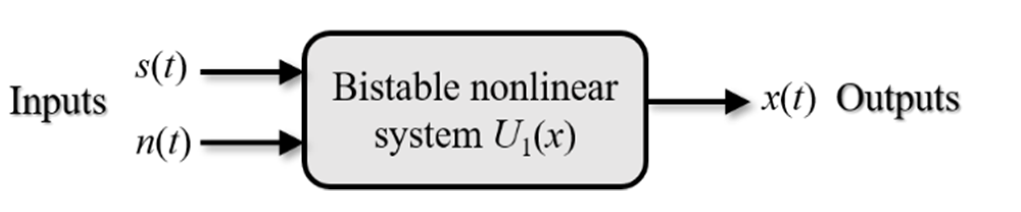
2. The SR Algorithm

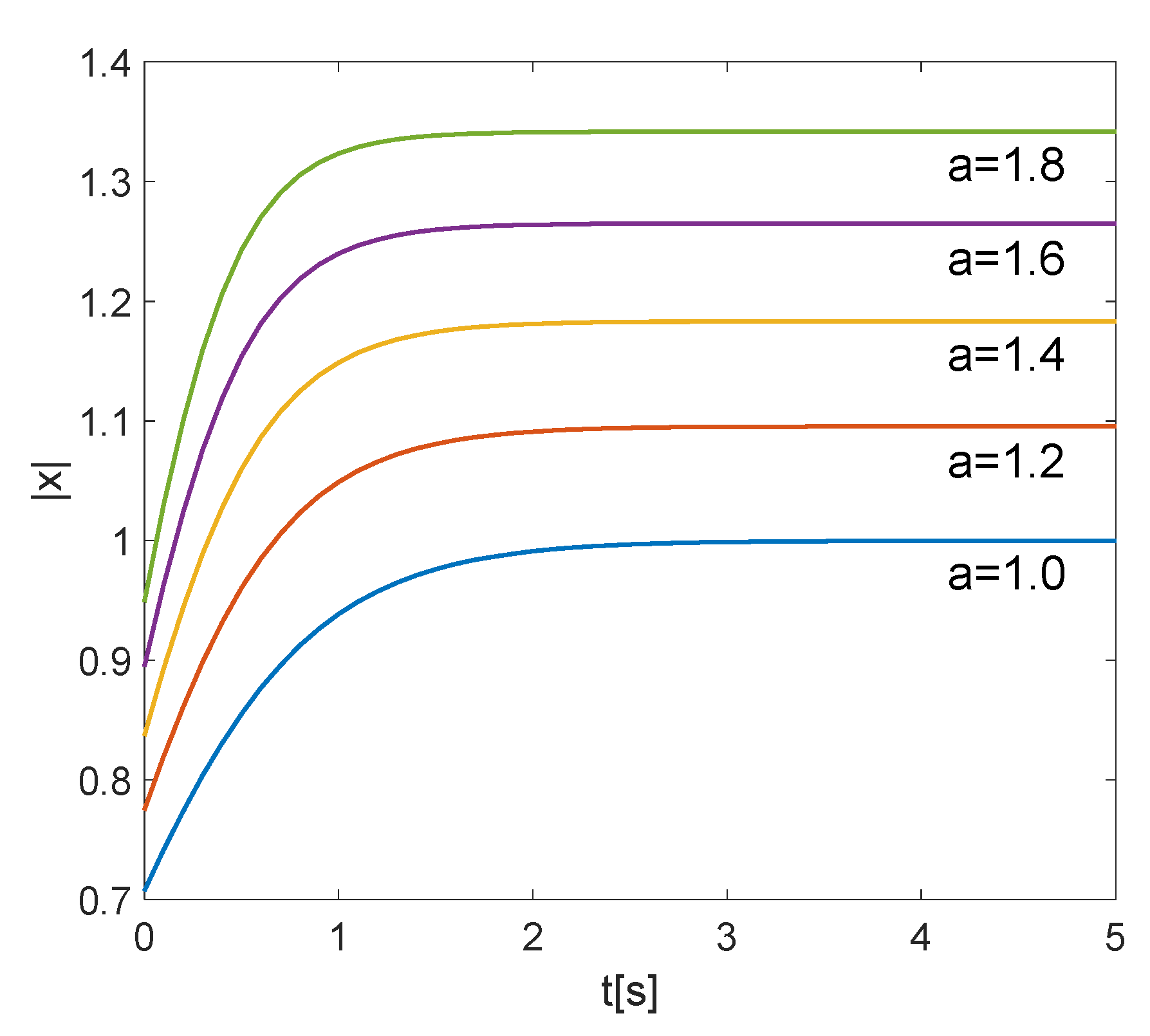
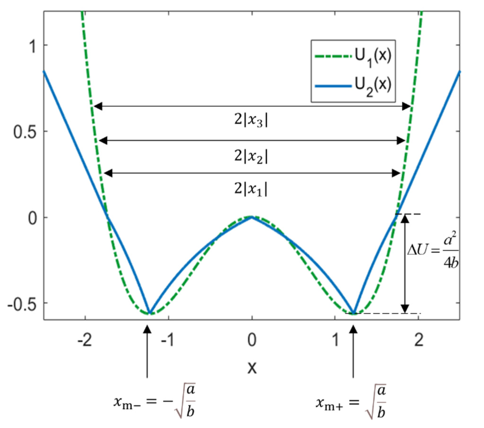
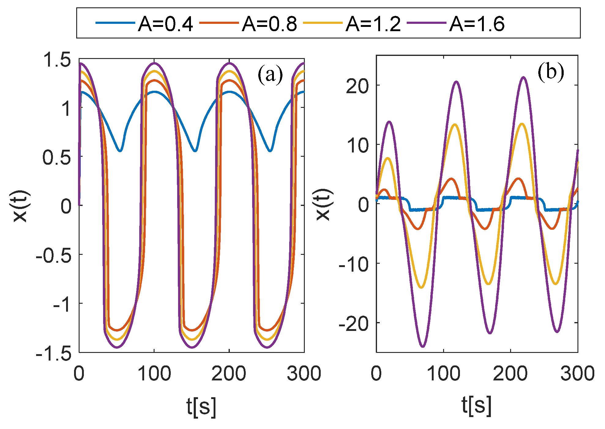
2.1. Classical SR and Output Saturation

Classical bistable stochastic resonance (CBSR) is a common SR. The framework of CBSR is shown in Figure 1. The outputs of CBSR are described by the following Langevin equations [24]:

$$\frac{dx}{dt}=-\frac{d{U}_1(x)}{dx}+s(t)+n(t)$$

(1)

$$U_1(x)=-\frac{a}{2}{x}^2+\frac{b}{4}{x}^4,a>0,b>0$$

(2)

where $s(t)=A\cos (2\pi ft)$ is the input signal, $A$ is the amplitude of the weak periodic signal, $f$ is the useful frequency, $U_1(x)$ is the system potential function, $a$ and $b$ are the system parameters, and $n(t)$ is the sum of the noise from the input signal $n_1(t)$ and excitation noise $n_2(t)$. $n(t)$ denotes a zero-mean. Gaussian white noise satisfies

$$\{\begin{array}{c}\langle n(t)\rangle =0\\ \langle n(t)n(t+\tau )\rangle =2D\delta (\tau )\end{array}$$

(3)

where $\tau$ is the time interval and $D$ is the noise intensity.

The outputs of CBSR can be written as:

$$\frac{dx}{dt}=ax-b{x}^3+A\cos (2\pi ft)+\sqrt{2D}\xi (t)$$

(4)

where $\xi (t)$ is the Gaussian white noise with a zero mean and unit variance.

CBSR can be explained by the Lorentzian distribution property that concentrates most of the noise energy into the low-frequency region. The SR phenomenon is suitable for controlling the low-frequency signal ($f\ll 1\mathrm{Hz}$). To deal with the high-frequency signal, Leng et al. [25] proposed a rescaling frequency (RF) SR by selecting a proper frequency–scale ratio, $R$. In this paper, we use the RF to handle the large parameter signals.

If we posit that there are no input signals and no noise, we obtain:

$$x=\pm \sqrt{\frac{a\exp (2at)}{1+b\exp (2at)}}$$

(5)

From Equation (5), we observed that the saturation phenomenon of output signal $x$ occurs when time, $t$, increases. As shown in Figure 2, the amplitude of the output signal is affected by the system parameters $a$ and $b$. The saturation state is ${\lim }_{t\to +\infty }x=\pm \sqrt{a/b}$, and $\left|x\right|$ is limited between $\sqrt{a/(1+b)}$ and $\sqrt{a/b}$ by the calculation. Output saturation is an inherent characteristic of CBSR, which is not affected by the input signal and noise. The steep barrier wall of the potential well is the cause of output saturation. When the saturation phenomenon occurs, the output signal of SR is the local optimal solution, which limits the weak signal detection performance of the system.

2.2. UBSR

To avoid the inherent output saturation of CBSR, we designed an unsaturated potential function structure by adjusting the slope of the barrier wall. UBSR consists of two parts: the linear potential function and the nonlinear potential function. The value of the output signal changes linearly when $x>c$ and $x<-c$ in the linear potential function. To handle the small-amplitude signal, the output should more easily oscillate in the two potential wells. The nonlinear parts adjust the slope of the potential function by using the exponential function. For comparison, UBSR and CBSR had the same barrier height, $\Delta U$, and well width, $x_m$.

The potential function of UBSR is:

$$U_2(x)=\{\begin{array}{ccc}-\frac{a^2}{4b}\left(\frac{x+c}{c-\sqrt{a/b}}\right)& when& x<-c\\ -\frac{a^2}{4b}\left[\frac{\exp (x+c)-1}{\exp (c-\sqrt{a/b})-1}\right]& when& -c\le x\le -\sqrt{a/b}\\ -\frac{a^2}{4b}\left[\frac{\exp (-x)-1}{\exp (\sqrt{a/b})-1}\right]& when& -\sqrt{a/b}<x<0\\ -\frac{a^2}{4b}\left[\frac{\exp (x)-1}{\exp (\sqrt{a/b})-1}\right]& when& 0\le x<\sqrt{a/b}\\ -\frac{a^2}{4b}\left[\frac{\exp (-x+c)-1}{\exp (c-\sqrt{a/b})-1}\right]& when& \sqrt{a/b}\le x\le c\\ \frac{a^2}{4b}\left(\frac{x-c}{c-\sqrt{a/b}}\right)& when& c<x\end{array}$$

(6)

Although Equation (6) is a complex expression, the complexity of the proposed method increased slightly because we used the fourth-order Runge–Kutta method to solve Equation (1). From Figure 3, the difference between two potential function curves of CBSR and UBSR can be observed. Two potential wells with minima were located at $x_m=\pm \sqrt{a/b}$ and the barrier height was $\Delta U=a^2/\left(4b\right)$. Due to the trend in the potential function of CBSR to be steep when $\left|x\right|>\sqrt{a/b}$, the amplitude of the output signal $\left|x_1\right|,\left|x_2\right|,\left|x_3\right|$ increases slowly and tends to a stable value gradually, which limits the signal enhancement ability of the CBSR. For UBSR, the amplitude of the output signal was unlimited and increased linearly; thus, UBSR avoided output saturation.

When the noise intensity is zero, the input signal frequency is 0.01 Hz, the system parameters satisfy $a=b=1$, and the sampling frequency is 5 Hz, the output curves of CBSR and UBSR for different values of amplitude $A$ are as shown in Figure 4.

The results demonstrate the relationship between the potential function and the amplitude of the output signal. Figure 4a demonstrates that the amplitude of the output signal $x$ increases with the amplitude of the input signal $A$ and gradually reaches saturation. Under the same conditions, the output amplitude of UBSR is higher than the output amplitude of CBSR. When the amplitude $A$ is small, such as $A=0.4$, Figure 4a shows that the output signals are restricted to one of two potential wells, but the output oscillates between two potential wells (Figure 4b). Thus, the experimental results indicated that the proposed UBSR method avoids output saturation, has larger output amplitude, and has more evident periodicity.

2.3. AUBSR

For strong noise, it is difficult to promote the occurrence of SR only by increasing the noise intensity, and it is necessary to adjust the parameters of UBSR adaptively. A genetic algorithm (GA) [15] adopts a “survival-of-the-fittest” strategy and can obtain a globally optimal solution. To quickly obtain the optimal parameters, we propose AUBSR by using the GA. The parameters $a$ and $b$ determine the barrier height and well width of the unsaturated potential function. The iteration step $h$ in the Runge–Kutta algorithm reflects the distance difference between the two adjacent signals. Therefore, the parameters $a$, $b$, and $h$ need to be optimized. For the GA, the necessary parameters are initialized using binary encoding. The length of the encoding is 40; the parameter ranges are $\left[a_{\min },a_{\max }\right]=\left[0.1,10\right]$, $\left[b_{\min },b_{\max }\right]=\left[0.1,10\right]$, and $\left[h_{\min },h_{\max }\right]=\left[0.1,0.5\right]$; the probability of selection, crossover, and mutation are 0.2, 0.5, and 0.05, respectively, and the maximum iteration is 1000, considering the fitness function as the basis of the three operations that affected the optimization direction and convergence speed of the overall algorithm. The output SNR is a common fitness index used to measure the performance of SR. However, it is difficult to measure the periodicity of the output signal and the accuracy of the target frequency at the same time. Therefore, we constructed a synthetic index (SI) to judge the performance of the output signal.

As the zero-crossing ratio (ZCR) measures the periodicity of the output signal and the structural correlation coefficient (SCC) evaluates the accuracy of the detective frequency, an index SI combining the advantages of the ZCR and the SCC is proposed. As the ZCR and the SCC have the best performance at one, it is easy to judge whether SR occurs according to the value of the SI. The equation of the SI can be expressed as:

$$SI=ZCR\times SCC$$

(7)

The ZCR is defined as the ratio of the actual number of the signal to the theoretical number of zero-crossings [16]. The ZCR (Algorithm 1) is described as follows:

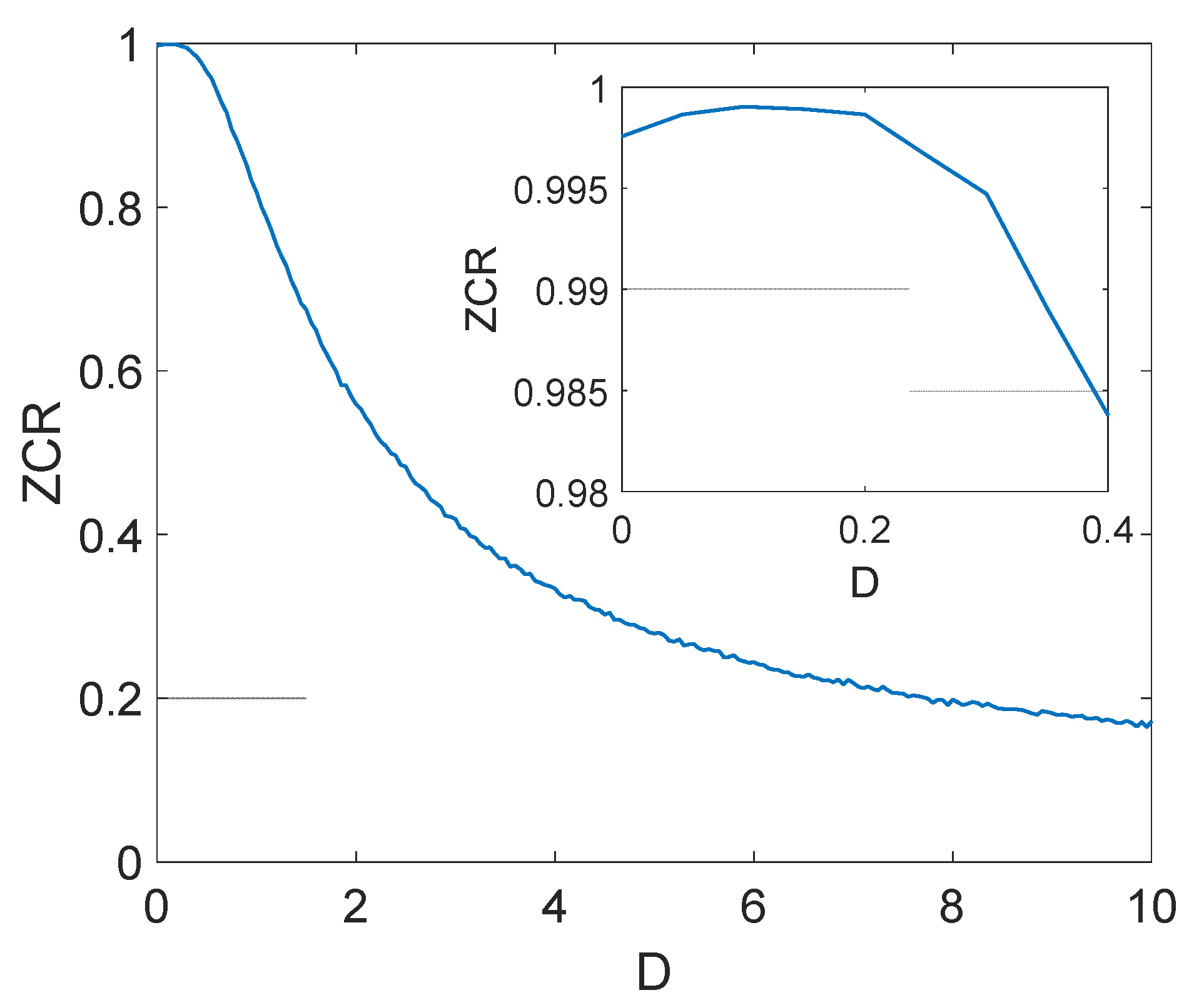
Algorithm 1. ZCR.

(1) Find the zero-crossing pairs $\left\{H(j),j=1,2,\dots ,M\right\}$ from the output sequence $\left\{x\left(k\right),k=1,2,\dots ,N\right\}$ subject to $x(k_j)\times x(k_j+1)<0$.

$H(j)=\left\{x(k_j),x(k_j+1),1\le k_j\le N\right\}$

where $M$ is the number of data pairs;

(2) Calculate the location $t$ of the zero point between the pairs $\left\{x(k_j),x(k_j+1)\right\}$ using linear interpolation.

$t_j=t_{k_j}+\frac{\left|x(k_j)\right|/f_s}{\left|x(k_j)\right|+\left|x(k_j+1)\right|}$

where $t_{k_j}$ is the location corresponding to $x(k_j)$ and $f_s$ denotes the sampling frequency;

(3) Calculate the zero-crossing spacing, $Z$, as follows:

$Z_j=t_{j+1}-t_j,1\le j\le M-1$.

(4) Remove the pseudo-zero-crossing points when $Z_j$ satisfies the following conditions

$\{\begin{array}{c}{Z}_j<\left(1-K\right)/\left(2f_{\max }\right)\\ Z_j>\left(1+K\right)/\left(2f_{\max }\right)\end{array},1\le j\le M-1$

where $f_{\max }$ is the frequency at the highest spectrum peak of the output signal, and the expected $Z_j$ is $1/\left(2f_{\max }\right)$. $K$ is an adjustable parameter, and the range is between 0 and 1.

(5) Calculate the ZCR as follows:

$ZCR=\frac{Num\times f_s}{2N\times f_{\max }-f_s}$

where $Num$ is the actual zero-crossing point, which can be calculated by removing the pseudo-zero-crossing points.

Significantly, the variable $K$ affects the number of zero-crossing points. A few zero-crossing points caused by noise are retained when $K$ is larger. Actual zero-crossing points caused by the periodic signal are partly be removed when $K$ is smaller. To ensure the periodicity of the output signal, the value range of $K$ is $0.2~0.4$ [16]. In this paper, we suppose that $K$ is 0.3. Figure 5 shows the trend in the ZCR versus the noise intensity, $D$. We observed that the closer to 1 the ZCR is, the more obvious the periodicity of the output signal is.

An SCC can evaluate the similarity between the target signal $S\left(k\right)$ and the output signal $X\left(k\right)$ in the frequency domain [26], which can be defined as follows (Algorithm 2):

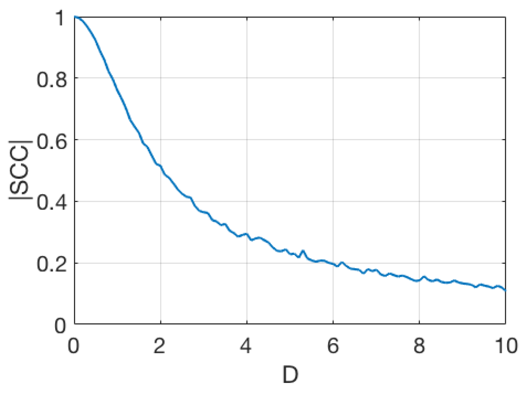
Algorithm 2. SCC.

(1) Calculate the frequency spectrum of the target signal and the output signal with a Fourier transform to obtain $\widehat{S}\left(k\right)$ and $\widehat{X}\left(k\right)$.

(2) Calculate the SCC as follows:

$SCC=\frac{{\displaystyle \sum {}_{k=1}^{N/2}\left[\widehat{S}\left(k\right)-\overline{S}\right]\left[\widehat{X}\left(k\right)-\overline{X}\right]}}{\sqrt{{\displaystyle \sum {}_{k=1}^{N/2}{\left[\widehat{S}\left(k\right)-\overline{S}\right]}^2}{{\displaystyle \sum {}_{k=1}^{N/2}\left[\widehat{X}\left(k\right)-\overline{X}\right]}}^2}}$

where $\overline{S}$ and $\overline{X}$ are the statistical mean values of $\widehat{S}\left(k\right)$ and $\widehat{X}\left(k\right)$, respectively.

We calculated that the value range of the SCC satisfied $0\le \left|\mathrm{SCC}\right|\le 1$ using the Schwartz inequality. The trend of the SCC versus the noise intensity $D$ without the SR system is shown in Figure 6. As shown in Figure 6, we observed that the larger the SCC is, the more similar the frequency spectrum of the two signals is. In SR, the closer the value of the SCC to 1, the better.

In summary, the SI has a fixed range of values, and the closer the value is to 1, the more accurate the algorithm performance. The SI satisfies the fitness function conditions such as non-negative, continuous, and maximized. Therefore, we can maximize the SI as the objective function of the GA.

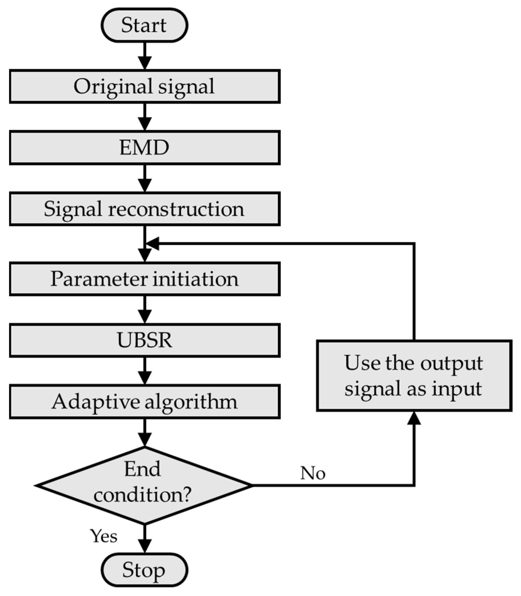
3. EMD-AUBSR

In practical applications, it is difficult to detect multi-frequency weak signals with strong background noise at the same time. It is also difficult to detect the target signals by using EMD or SR alone. Therefore, we constructed EMD-AUBSR for the detection of multi-frequency weak signals by combining the advantages of EMD and UBSR. Figure 7 shows the algorithm flow chart.

EMD-AUBSR preprocesses the original input signal by using EMD, then detects a weak signal by AUBSR. The main steps of the proposed EMD-AUBSR method are described as follows:

(1)

Original Signal:

For multi-frequency signals detection, the input signal is defined as the classic form of the addition of two cosine signals [27].

$$s(t)=A_1\cos (2\pi f_{1}t)+A_2\cos (2\pi f_{2}t)$$

(8)

where $A_1=0.2$, $f_1=100\mathrm{Hz}$, $A_2=0.1$, and $f_2=200\mathrm{Hz}$. The noise at the input is Gaussian white noise.

In practical applications, the form of the signal is diverse and the signals have a certain bandwidth. As the actual signal can be regarded as a combination of multiple cosine signals, for a comparison to other methods, the input signal is usually set as two cosine signals with narrow bandwidths.

(2)

EMD:

EMD is an adaptive time-frequency decomposition algorithm with no prior knowledge. The complex signal can be decomposed into several IMFs and the residual error through EMD. Each IMF represents a signal with a frequency only at a certain moment, which provides the actual physical meaning of the instantaneous frequency. Each IMF must meet the following two conditions [28]:

• The numbers of zero-crossings and extreme points of the entire signal are equal or differ by at most 1;
• At any point of the signal, the mean value of the envelope is composed of local maximum points, and the local minimum point is equal to zero.

For the original signal sequence $x(t)$, the flow of EMD decomposition is as follows (Algorithm 3).

Algorithm 3. EMD.

(1) Obtain the local maximum points and the minimum points of the signal in the time domain. We obtain the upper envelope $e^u(t)$ and the lower envelope $e^l(t)$ using the cubic spline interpolation. Calculate the mean value of the envelope $m(t)$ as follows:

$m(t)=\frac{e^u(t)+e^l(t)}{2}$

(2) Calculate $h_1(t)=x(t)-m(t)$. Discontinue this step if $h_1(t)$ meets the two conditions of IMF. Otherwise, let $p(t)$ be equal to the last output and repeat equation $h_{1k}(t)=p(t)-m(t)$ $k$ times until $h_{1k}(t)$ meets the conditions.

(3) Let $c_1(t)=h_{1k}(t)$. Calculate the residual signal $r_1(t)$

$r_1(t)=x(t)-c_1(t)$

(4) Repeat steps (1) to (3) until the final sequence $r_N(t)$ meets terminate condition

$r_i(t)=r_{i-1}(t)-c_i(t),i=2,3,\dots ,N$.

(5) The results of EMD can be expressed as

$x(t)={\displaystyle {\displaystyle \sum }_{i=1}^N{c}_i(t)}+r_N(t)$

EMD uses the local fluctuation signal and decomposes the original signal into a series of frequency components from a high to low frequency. We can retain useful IMF components based on the known target frequency. The accuracy of the subsequent AUBSR detection is enhanced by the preprocessing operations.

(3)

AUBSR

Firstly, determine the system parameter group, $\left[a,b,h\right]$, which needs to be optimized, and then encode them according to the settings in Section 2.3. Second, as the subsequent operations are based on the individual fitness value, a new fitness function SI is constructed and $\max \left\{SI\right\}$ is used as the objective function of the adaptive algorithm. Third, according to the preset probability factor and the calculated fitness value, three operations of selection, crossover, and mutation are performed on the current generation to obtain a better new generation. Finally, the algorithm gradually converges after a constant iteration. Until the maximum number of iterations is met, the optimal parameter group corresponding to the maximum fitness value is obtained, thereby obtaining the optimal output signal.

4. Experimental Results and Analysis

In this section, the results of several experiments are described. Firstly, we compare the performance of the novel index SI to the SNR and illustrate the effectiveness of AUBSR with strong background noise in a single-frequency signal. Then, the experimental results demonstrate that EMD-AUBSR can detect multi-frequency signals.

4.1. Single-Frequency Weak Signal Detection

The output SNR is a common performance index of SR. To illustrate the higher accuracy of the proposed fitness function SI, we set $\max \left\{SNR\right\}$ and $\max \left\{SI\right\}$ as the objective functions for the control experiments. The output SNR is calculated as

$$SNR=10\lg \left(\frac{SP}{NN-SP}\right)$$

(9)

where $SP={\left|x(k)\right|}^2$ denotes the output signal power, $x(k)$ is the amplitude at $f$ in the response spectrum, and $NN={\displaystyle {\displaystyle \sum }_{j=1}^{N/2}{\left|x(k)\right|}^2}$ is the total power of the signal and noise.

The frequency of the periodic signal is $f=0.01\mathrm{Hz}$ and the amplitude $A=0.35$. The sampling frequency is $f_s=5\mathrm{Hz}$, and the data length is $N=4096$. The system parameters are $a=2$ and $b=1$. The noise intensity $D$ is increased from 0.1 to 10. The output SNR is the average of running each noise intensity 500 times.

Figure 8a shows the output SNR curves of the two systems with noise intensity $D$. The two curves are non-monotonic and reached the maximum when $D$ was approximately $0.4~0.7$ because of the occurrence of SR. When $D>0.7$, the experimental results of UBSR decreased at a slower speed than CBSR. Notably, the SNR of the UBSR system was always higher than that of the other system, which indicated that the performance of this algorithm is more accurate. In practical applications, it is difficult to judge whether SR occurs from the value of the SNR. Thus, an SI with a fixed range was constructed to measure the output result. Figure 8b shows the SI curves of the two SR algorithms under the same conditions. From Figure 8b, we observed that the maximum of the SI was close to one and the minimum of the SI was close to zero. This conclusion is consistent with the value range when SI is [0, 1]. We observed that SR occurred in the narrow range nearby the peak; therefore, it was easier to judge whether SR had occurred. We believe that SR occurred when the SI was larger than the experiential value $\mathrm{SI}=0.5$.

For weak signal under a strong background noise, we adjusted the relevant parameters of SR to promote its occurrence. For this reason, we constructed AUBSR. The noise intensity $D=10$ and the initial group $\left[a,b,h\right]$ had random values. Figure 9 shows the output signals of AUBSR using $\max \left\{SNR\right\}$ and $\max \left\{SI\right\}$ as the objective functions. After several iterations, the optimal system parameter groups of the two algorithms were $\left[a_{SNR},b_{SNR},h_{SNR}\right]=\left[4.2475,1.4155,0.0881\right]$ and $\left[a_{SI},b_{SI},h_{SI}\right]=\left[9.6894,6.1096,0.0551\right]$. The output SNR of AUBSR increased to −4.7 dB. The SI increased to 0.56. From Figure 9b, we observed that the output signal waveform was more periodic, and the output signal spectrum at the target frequency was clearer. Thus, we calculated that utilizing the SI as a fitness function benefited SR to measure the periodicity of the output signal and the accuracy of the detective frequency at the same time. In future studies, we can also optimize the system performance by setting a suitable threshold of the SI.

4.2. Multi-Frequency Weak Signals Detection

According to adiabatic approximation theory, the input signal of SR needs to meet the limitation of small parameters, which means that the input signal has a low frequency, small amplitude, and low noise intensity. However, big parameters problem may be involved in signal detection. In this section, we used RF to solve the high-frequency problem and EMD-AUBSR to detect multi-frequency signals. The rescaling ratio is $R=\mathrm{10,000}$. The sampling frequency was 15 kHz and the length of the signal was 4096 points.

When the noise intensity was small, such as $D=1$, eight IMF components after EMD could be obtained, as shown in Figure 10. From IMF4 and IMF5 in Figure 10b, we observed that the output spectrum had peak values at the frequencies of the two target signals, which indicated that the two target signals could be successfully separated by EMD alone. When the noise intensity increased to 10, the EMD decomposition result (Figure 11) was difficult to distinguish between the two target signals. The proposed EMD-AUBSR solved this problem. We chose the IMF component closest to the target frequency as the input signal of AUBSR. The input was the sum of IMF3 to IMF6. After a continuous iteration, the optimal parameter group of the algorithm was obtained through the adaptive algorithm.

The parameter settings of the GA were the same as in Section 2.3, and we adopted $\max \left\{SI\right\}$ as the fitness function. The initial parameter group was randomly selected within the preset range. The results of EMD-ACBSR and EMD-AUBSR are shown in Figure 12 after 1000 iterations.

As shown in Figure 12a, a signal with a lower frequency $f_1=100\mathrm{Hz}$ was obtained, and the higher frequency $f_2=200\mathrm{Hz}$ was submerged in clutter through EMD-ACBSR. Figure 12b shows that the proposed algorithm successfully detected the two target signals. The clutter component in Figure 12b is less than that in Figure 12a. The performance index SI eventually increased to 0.63, which is greater than the preset 0.5; therefore, SR occurred at this time. The optimal system parameter group of EMD-AUBSR is $\left[a_{opt},b_{opt},h_{opt}\right]=\left[3.5724,5.3119,0.0362\right]$. The amplitude of the frequency spectrum in Figure 12b is larger than that in Figure 12a, which is also consistent with the results shown in Figure 4 and Figure 9. This is because the proposed algorithm avoids output saturation and increases the amplitude of the output signal. The SR phenomenon more easily occurs in the improved EMD-AUBSR based on the above analysis. The experimental results showed that EMD-AUBSR is more accurate than EMD-ACBSR at multi-frequency weak signals detection.

5. Conclusions

In this paper, EMD-AUBSR was proposed to detect a multi-frequency weak signal. Our algorithm highlights the following three points:

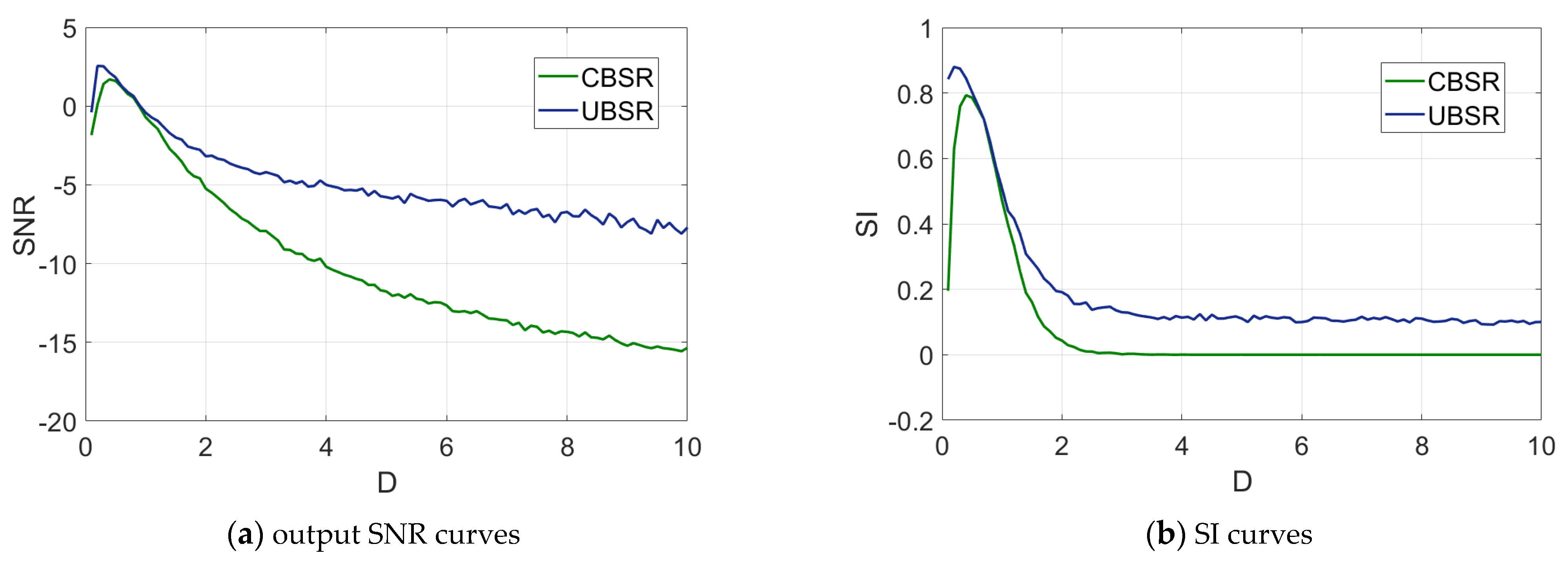
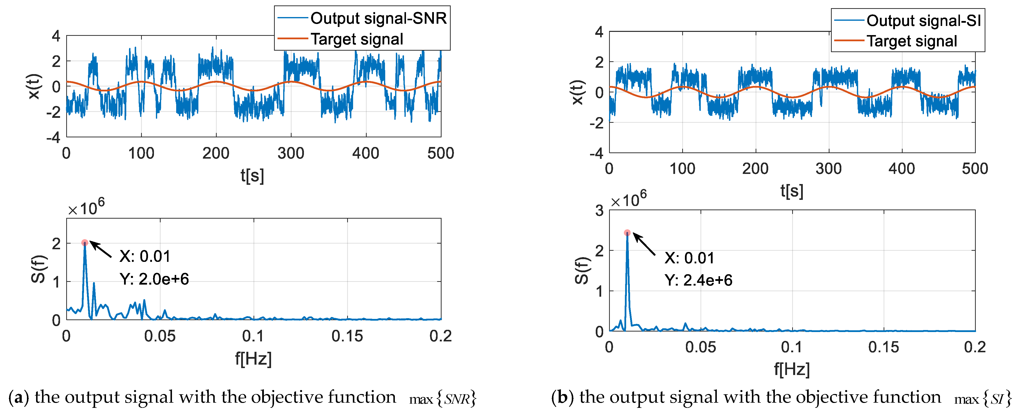
• For the inherent output saturation of CBSR, we designed an unsaturated potential function structure to overcome this defect and built an SI to measure algorithm performance accurately in AUBSR.
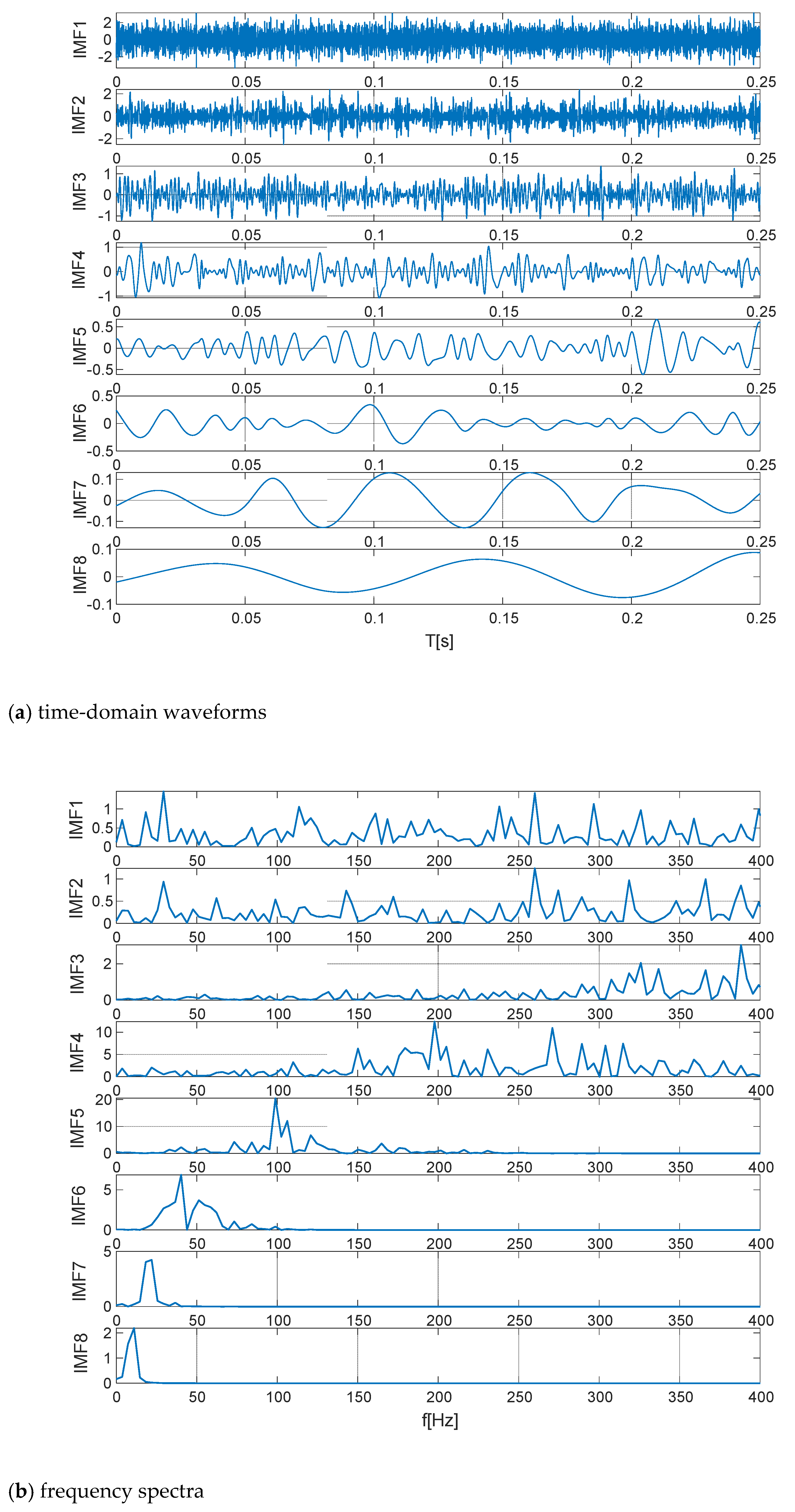
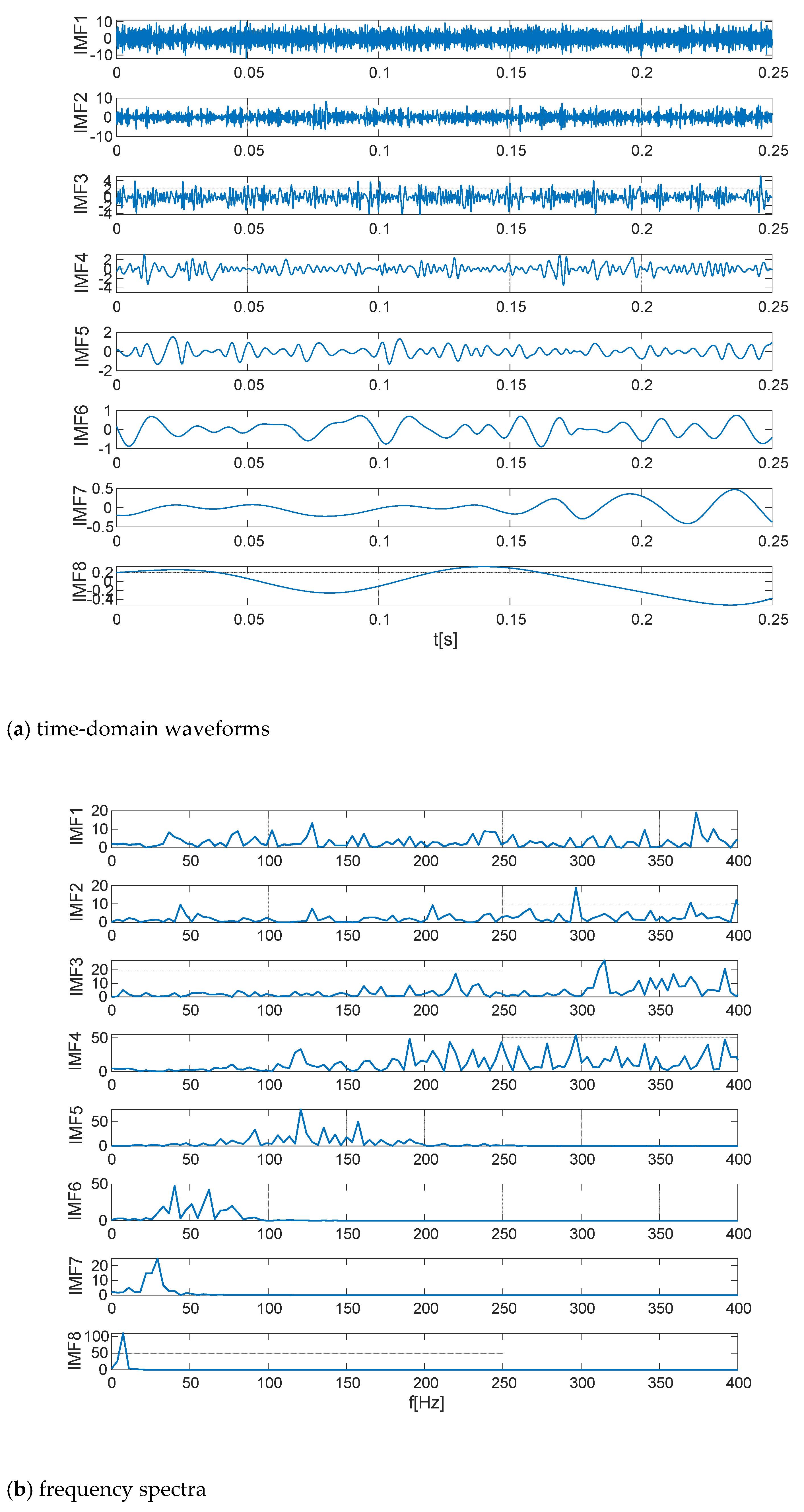
• EMD can detect multi-frequency signals when the noise intensity is low, but mode aliasing occurs when the noise is strong. We constructed EMD-AUBSR due to the advantages of UBSR to decrease mode mixing of EMD. The experimental results prove this aspect.
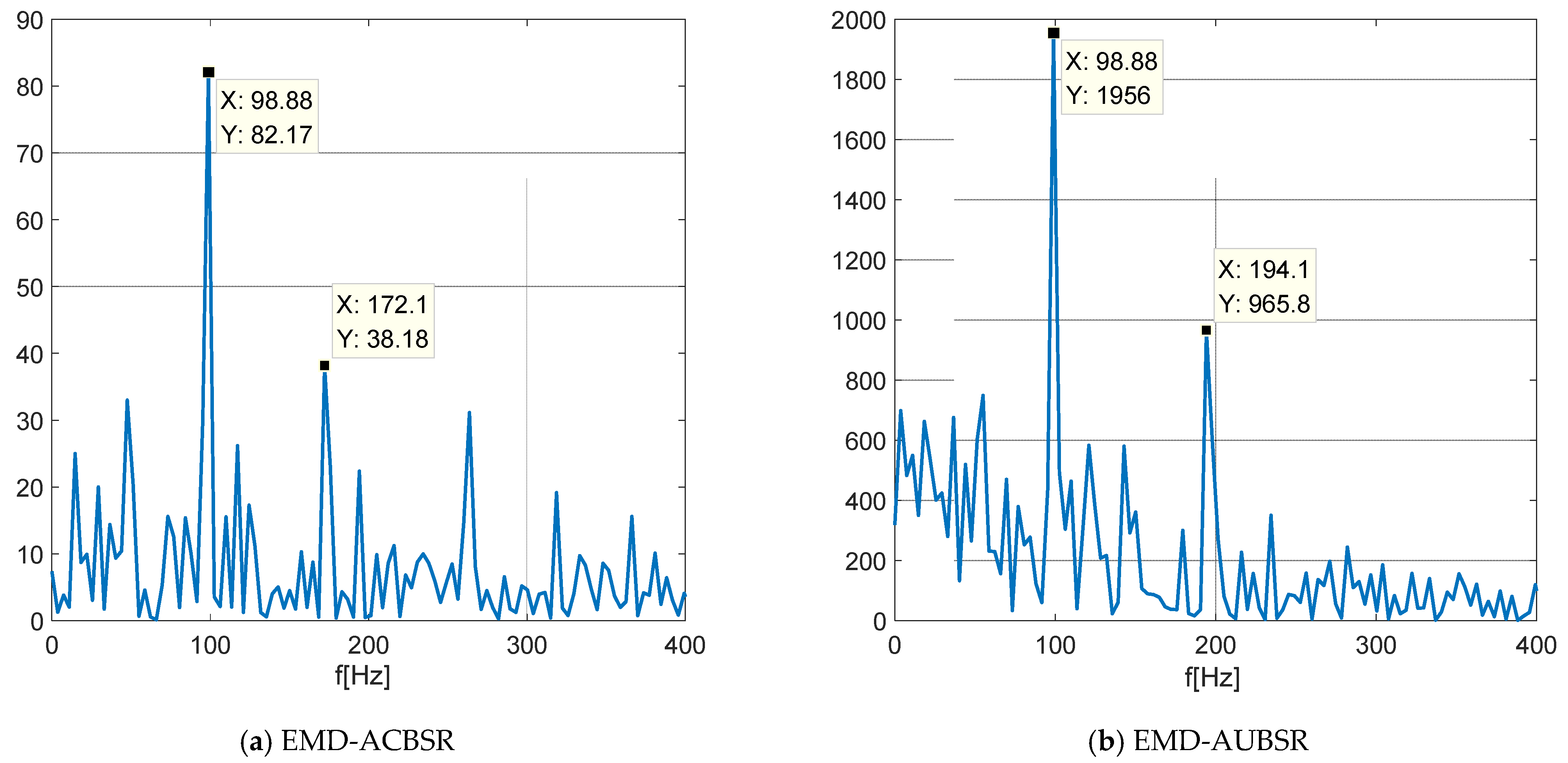
• EMD-AUBSR is effective for detecting multi-frequency signals under strong noise, whereas EMD and AUBSR alone cannot.

Future research directions include studying different multi-frequency signals decomposition techniques based on SR such as VMD and HVD, adding delay feedback to further optimize the SR structure, and increasing the simulation of actual signals with a certain bandwidth.

References

- He, K.; Xia, Z.; Si, Y.; Lu, J. Noise reduction of welding crack AE Signal based on EMD and wavelet packet. Sensors 2020, 20, 761. [Google Scholar] [CrossRef] [Green Version]
- Shi, H.; Guo, J.; Yuan, Z.; Liu, Z. Incipient fault detection of rolling element bearings based on deep EMD-PCA algorithm. Shock. Vib. 2020, 2020, 8871433. [Google Scholar] [CrossRef]
- Abbate, A.; Koay, J.; Frankel, J.; Schroeder, S.C.; Das, P. Signal detection and noise suppression using a wavelet transform signal processor: Application to ultrasonic flaw detection. IEEE Trans. Ultrason. Ferroelectr. Freq. Control 1997, 44, 14–26. [Google Scholar] [CrossRef] [PubMed]
- Qin, Y.; Tang, B.; Wang, J. Higher-density dyadic wavelet transform and its application. Mech. Syst. Signal Process. 2010, 24, 823–834. [Google Scholar] [CrossRef]
- Cheng, Y.; Chang, Q. A coarse-to-fine adaptive Kalman filter for weak GNSS signals carrier tracking. IEEE Commun. Lett. 2019, 23, 2348–2352. [Google Scholar] [CrossRef]
- Benzi, R.; Sutera, A.; Vulpiani, A. The mechanism of stochastic resonance. J. Phys. A Math. Gen. 1981, 14, 453–457. [Google Scholar] [CrossRef]
- Hari, V.; Anand, G.; Premkumar, A.B.; Madhukumar, A. Design and performance analysis of a signal detector based on suprathreshold stochastic resonance. Signal Process. 2012, 92, 1745–1757. [Google Scholar] [CrossRef]
- Wang, S.; Wang, F.; Wang, S.; Li, G. Detection of multi-frequency weak signals with adaptive stochastic resonance system. Chin. J. Phys. 2018, 56, 994–1000. [Google Scholar] [CrossRef]
- McNamara, B.; Wiesenfeld, K. Theory of stochastic resonance. Phys. Rev. A 1989, 39, 4854–4869. [Google Scholar] [CrossRef]
- He, Q.B.; Wang, J. Effects of multiscale noise tuning on stochastic resonance for weak signal detection. Digit. Signal Process. 2012, 22, 614–621. [Google Scholar] [CrossRef]
- Ren, R.B.; Luo, M.K.; Deng, K. Stochastic resonance in a fractional oscillator subjected to multiplicative trichotomous noise. Nonlinear Dyn. 2017, 90, 370–390. [Google Scholar] [CrossRef]
- Shi, P.; Yuan, D.; Han, D.; Zhang, Y.; Fu, R. Stochastic resonance in a time-delayed feedback tristable system and its application in fault diagnosis. J. Sound Vib. 2018, 424, 1–14. [Google Scholar] [CrossRef]
- Qin, Y.; Tao, Y.; He, Y.; Tang, B. Adaptive bistable stochastic resonance and its application in mechanical fault feature extraction. J. Sound Vib. 2014, 33, 7386–7400. [Google Scholar] [CrossRef]
- Liu, X.; Liu, H.; Yang, J.; Litak, G.; Cheng, G.; Han, S. Improving the bearing fault diagnosis efficiency by the adaptive stochastic resonance in a new nonlinear system. Mech. Syst. Signal Process. 2017, 96, 58–76. [Google Scholar] [CrossRef]
- Zhou, P.; Lu, S.; Liu, F.; Liu, Y.; Li, G.; Zhao, J. Novel synthetic index-based adaptive stochastic resonance method and its application in bearing fault diagnosis. J. Sound Vib. 2017, 391, 194–210. [Google Scholar] [CrossRef]
- Li, J.; Zhang, J.; Li, M.; Zhang, Y. A novel adaptive stochastic resonance method based on coupled bistable systems and its application in rolling bearing fault diagnosis. Mech. Syst. Signal Process. 2019, 114, 128–145. [Google Scholar] [CrossRef]
- Xu, B.; Li, J.; Duan, F.; Zheng, J. Effects of colored noise on multi-frequency signal processing via stochastic resonance with tuning system parameters. Chaos Solitons Fractals 2003, 16, 93–106. [Google Scholar] [CrossRef]
- Lu, Z.; Yang, T.; Zhu, M. Study of the method of multi-frequency signal detection based on the adaptive stochastic resonance. Abstr. Appl. Anal. 2013, 2013, 360–374. [Google Scholar] [CrossRef] [Green Version]
- Shi, P.; Ding, X.; Han, D. Study on multi-frequency weak signal detection method based on stochastic resonance tuning by multi-scale noise. Measurement 2014, 47, 540–546. [Google Scholar] [CrossRef]
- Gong, S.; Li, S.; Wang, H.; Ma, H.; Yu, T. Multi-frequency weak signal detection based on wavelet transform and parameter selection of bistable stochastic resonance model. J. Vib. Eng. Technol. 2021, 1–20. [Google Scholar] [CrossRef]
- Civera, M.; Surace, C. A comparative analysis of signal decomposition techniques for structural health monitoring on an experimental benchmark. Sensors 2021, 21, 1825. [Google Scholar] [CrossRef] [PubMed]
- Wu, Z.; Huang, N.E. Ensemble empirical mode decomposition: A noise-assisted data analysis method. Adv. Adapt. Data Anal. 2011, 1, 1–41. [Google Scholar] [CrossRef]
- Yeh, J.R.; Shieh, J.S.; Huang, N.E. Complementary ensemble empirical mode decomposition: A novel noise enhanced data analysis method. Adv. Adapt. Data Anal. 2010, 2, 135–156. [Google Scholar] [CrossRef]
- Gammaitoni, L.; Marchesoni, F.; Menichella-Saetta, E.; Santucci, S. Stochastic Resonance in Bistable Systems. Phys. Rev. Lett. 1989, 62, 349–352. [Google Scholar] [CrossRef]
- Leng, Y.; Leng, Y.; Wang, T.; Guo, Y. Numerical analysis and engineering application of large parameter stochastic resonance. J. Sound Vib. 2006, 292, 788–801. [Google Scholar] [CrossRef]
- Xiao, K.; Zhou, Z. The EMD based on adaptive stochastic resonance for weak signal detection. In Proceedings of the 2016 Chinese Control and Decision Conference (CCDC), Yinchuan, China, 28–30 May 2016; pp. 2153–2157. [Google Scholar]
- Li, G.; Li, J.; Wang, S.; Chen, X. Quantitative evaluation on the performance and feature enhancement of stochastic resonance for bearing fault diagnosis. Mech. Syst. Signal Process. 2016, 81, 108–125. [Google Scholar] [CrossRef]
- Jiao, S.; Jiang, W.; Lei, S.; Huang, W. Research on detection method of multi-frequency weak signal based on stochastic resonance and chaos characteristics of duffing system. Chin. J. Phys. 2019, 64, 333–347. [Google Scholar]
Publisher’s Note: MDPI stays neutral with regard to jurisdictional claims in published maps and institutional affiliations. |
© 2021 by the authors. Licensee MDPI, Basel, Switzerland. This article is an open access article distributed under the terms and conditions of the Creative Commons Attribution (CC BY) license (https://creativecommons.org/licenses/by/4.0/).
Share and Cite
Cui, L.; Yang, J.; Wang, L.; Liu, H. Adaptive Unsaturated Bistable Stochastic Resonance Multi-Frequency Signals Detection Based on Preprocessing. Electronics 2021, 10, 2055. https://doi.org/10.3390/electronics10172055
Cui L, Yang J, Wang L, Liu H. Adaptive Unsaturated Bistable Stochastic Resonance Multi-Frequency Signals Detection Based on Preprocessing. Electronics. 2021; 10(17):2055. https://doi.org/10.3390/electronics10172055
Chicago/Turabian StyleCui, Lin, Junan Yang, Lunwen Wang, and Hui Liu. 2021. "Adaptive Unsaturated Bistable Stochastic Resonance Multi-Frequency Signals Detection Based on Preprocessing" Electronics 10, no. 17: 2055. https://doi.org/10.3390/electronics10172055