Wideband Frequency Invariant Array Synthesis Based on Matrix Singular Value Decomposition

Abstract

In this paper, an analytic method for frequency invariant (FI) array synthesis is proposed based on matrix singular value decomposition. By grouping the elements of FI array into a few subarrays, the FI pattern in the whole frequency band is realized. Using this algorithm, the number of sub arrays is reduced. Simulation results show that the proposed algorithm can synthesize the 64-element broadband FI array in 0.52 s. For the 18-element linear array, the half power beam width (HPBW) changes less than 0.6 degrees in the bandwidth. Moreover, the range of HPBW variation decreases rapidly along with the increase in the number of elements. Furthermore, the effectiveness of the algorithm is verified by synthesizing FI array with low side lobe level (SLL), beam scanning, and notch requirements. The examples in this paper show that the proposed algorithm can achieve better pattern characteristics with fewer elements. Finally, a broadband antenna with 2:1 bandwidth is improved, and two FI arrays of 23 elements and 64 elements are formed by using the antenna. The active pattern of the array element is introduced into the proposed algorithm, and two FI arrays synthesized by the algorithm are simulated by full wave software.

1. Introduction

With the development of wireless communication technology, array antenna, as one of the key forms of communication equipment, has attracted much attention. For some typical wideband signal processing equipment, such as sonar, underwater communication, target recognition, etc., the frequency invariant (FI) beam of wideband array can receive a wideband signal without distortion [1,2,3].

Compared with other array synthesis methods, the radiation pattern of FI array needs to be stable in a wide frequency band. As early as the 1970s, broadband FI pattern was realized through combination sub arrays of each frequency point [4,5,6]. When there are many operating frequency points, the array needs a large number of sensors. Ward et al. proposed a systematic design method based on the FI condition of the array response function [7,8]. Using this method, the FI pattern is realized by combining the main filters with the sub filters. The improvement of the accuracy of the FI beam depends on the sampling rate of the system. Boyd et al. introduced the convex optimization method into array synthesis [9,10,11], and proposed a frequency design method based on spatial response variation (SRV) constraint. Many iterative operations are needed in this method, and the amount of calculation is very large.

In order to reduce the amount of computation, Crocco et al. proposed the least square (LS) method of FI and directivity of reconfigurable pattern [12,13,14,15]. Ghavami et al. applied it to the design of the FI beam former with a narrow-band array structure [16]. Based on the Fourier transform relationship between the array weighting coefficient matrix and the pattern, the weighting coefficient of the beam former is obtained by the inverse fast Fourier transform (IFFT), which is further extended to the takeout delay line array [17,18] and the sensor delay line array [19,20] with uniform structure. A synthesis technique based on the matrix pencil method (MPM) is proposed by Y. Liu et al. to synthesize the FI arrays [21,22]. The simulated annealing (SA) technique and the weighted least-squares (WLS) are combined by W. Tang [23]. The weighting function values of FI array are calculated iteratively.

The synthesis of FI array can be classified into three categories: (1) the methods of analytic; (2) quasi analytic; and (3) optimization. The analytical method is fast and efficient, but it is not competent for the complex array form and special radiation direction constraints. The optimization algorithm has a wide range of applications, but its speed is slow, especially for large arrays. The quasi analytic method combines the advantages of the two methods, and has been widely concerned. Identifying methods to reduce the number of elements in the array, reduce the computational complexity of the algorithm, and improve the accuracy of pattern synthesis have become hot issues.

The singular value decomposition (SVD) is used by Y. Liu to reduce the number of elements in the array [24]. The SVD is applied to solve the problems of multi-beam directional modulation (DM) to reducing the complexity of multi-carrier frequency diverse array (FDA) [25]. In the array synthesis problems, SVD is mostly used to reduce the array complexity. In fact, the SVD of matrices in synthesis of antenna array contain a rich amount of information about the array. In this paper, the eigenvectors of the minimal singular values is used to obtain the excitations of subarray in FI array.

To validate the proposed algorithm, three cases are carried out by using 5 FI arrays composed of isotropic ideal point elements. These three cases apply the algorithm proposed to FI arrays with low side lobe level (SLL) and scanning and notch constraints, respectively. In order to introduce the influence of the variation of the element pattern in the bandwidth and the mutual coupling between the elements into the array synthesis algorithm, a broadband isotropic antenna is designed in this paper. In the fourth case, two FI arrays are composed of this antenna element. The full wave simulation results of two FI arrays further verify the effectiveness of the algorithm.

2. Materials and Methods

As shown in Figure 1, a uniformly spaced linear array is composed of N elements with a spacing of d.

Due to the symmetry of the linear array, only the radiation directionality of the array on the YOZ plane is considered here. The elevation range is [0,π]. M sampling angles are taken. Sampling angle interval is $\Delta \theta$.The array pattern can be obtained from the following formula:

$$S_l=P_l\cdot w_l$$

(1)

In the above formula, $S_l$ is the M-dimensional column vector ${\left(s(f_l,{\theta }_1),s(f_l,{\theta }_2),\cdots ,s(f_l,{\theta }_m),\cdots ,s(f_l,{\theta }_M)\right)}^T$. It represents the pattern of the array at the lth sampling frequency f_l. $w_l$ is N_l-dimensional column vector ${\left({\omega }_{1l},{\omega }_{2l},\cdots ,{\omega }_{nl},\cdots ,{\omega }_{Nl}\right)}^T$. It is the excitation vector of N_l array elements at the lth sampling frequency f_l0. $P_l$ is M × N_l -dimensional matrix.

$$\begin{gathered} P_l={[p_{mn}(f_l,{\theta }_m)]}_{M\times N_l}= \\ \left[\begin{array}{ccccc}{p}_1(f_l,{\theta }_1)& \cdots & p_n(f_l,{\theta }_1)e^{j{k}_l{d}_n\cos {\theta }_1}& \cdots & p_{N_l}(f_l,{\theta }_1)e^{j{k}_l{d}_{N_l}\cos {\theta }_1}\\ ⋮& & ⋮& & ⋮\\ p_1(f_l,{\theta }_m)& \cdots & p_n(f_l,{\theta }_m)e^{j{k}_l{d}_n\cos {\theta }_m}& \cdots & p_{N_l}(f_l,{\theta }_m)e^{j{k}_l{d}_{N_l}\cos {\theta }_m}\\ ⋮& & ⋮& & ⋮\\ p_1(f_l,{\theta }_M)& \cdots & p_n(f_l,{\theta }_M)e^{j{k}_l{d}_n\cos {\theta }_M}& \cdots & p_{N_l}(f_l,{\theta }_M)e^{j{k}_l{d}_{N_l}\cos {\theta }_M}\end{array}\right] \end{gathered}$$

(2)

For narrow-band arrays, the distortion of the pattern in the band is generally not considered. When the array works in the broadband, the beam will change obviously. As can be seen from Figure 2. The main lobe of pattern narrows with the increase in frequency, which affects the performance of wideband array. For broadband arrays, the FI method must be used.

In order to realize the FI pattern on broadband (f_b, f_u), the uniform array must face the change of the array aperture in broadband. Therefore, with the increase in frequency, the number of active elements in the array should be gradually reduced. Using the high-frequency array as a reference to design the uniform array will lead to a large number of array elements needed in the low-frequency array and will increase the complexity of the array. Using the low-frequency array as a reference design, the element spacing of the high-frequency array will increase, which will make it difficult to suppress the grating lobe of the antenna array.

In order to reduce the complexity of the array, a uniform linear array with a spacing of 0.5${\lambda }_1$ is established in this paper. ${\lambda }_1$ is the wavelength corresponding to frequency f₁(f₁ = f_b). The length of N-element linear array is:

$$A=\left(N-1\right)\times d$$

(3)

Considering the lth sampling frequency f_l, in order to ensure that the electrical length of the array at this frequency is invariant, it should meet the following requirements:

$$\left(N_l-1\right)\times \frac{d}{{\lambda }_l}\approx \left(N-1\right)\times \frac{d}{{\lambda }_1}$$

(4)

where N_l is the number of active elements of the array working at the lth sampling frequency f_l. When N_l ∈(N₁ = N, N₂ = (N − 1),…, N_L = (N – L + 1)), the lth sub array composed of N_l active elements in N-element uniform linear array will work in frequency band [f_l, f_l+1]. Further, we can obtain:

$$N_l-1\approx \left(N-1\right)\times \frac{{\lambda }_l}{{\lambda }_1}$$

(5)

From Equation (5), we can obtain the following equation:

$$f_l=\frac{N-1}{N_l-1}{f}_1$$

(6)

The working frequency band of all L sub arrays is (f₁, f_L+1), which will cover the bandwidth of the array (f_b, f_u).

Table 1. Active elements and BW of subarray in FI array.

Subarray	Active Elements								BW
F1	1	2	…	…	…	…	N − 1	N	[fb, f2)
F2	1	2	…	…	…	…	N − 1		[f2, f3)
.	.	.	…	…	…	…			.
Fl	1	2	…	…	Nl				[fl, fl+1)
.	.	.	…	…					.
FL	1	2	…	NL					[fL, fu]

shows the allocated band width (BW) and index number of active element in each sub array. The frequency f_l in Equation (2) is set as the central frequency of the working bandwidth of each sub array:

Once the number of effective elements of each sub array is determined, the equation that the sub array pattern synthesis should meet can be obtained as follows:

$$S_{\mathrm{D}}=P_l\cdot w_l$$

(7)

The M-dimensional column vector $S_{\mathrm{D}}$ is the desired pattern of the FI array. The WTLSM algorithm [26] can be used to solve Equation (7) for each sub array. The design process of the FI array is shown in Figure 3.

The procedure can be concluded as follows:

Step 1. The vector $S_{\mathrm{D}}={\left[s({\theta }_1),s({\theta }_2),\cdots ,s({\theta }_m),\cdots ,s({\theta }_M)\right]}^T$ is defined. $s({\theta }_m)$ is the desired pattern of the FI array at direction ${\theta }_m$.

Step 2. The parameters fb and fu are defined by the bandwidth of the FI array.

Step 3. The N is set as the element number of the FI array. The d is 0.5${\lambda }_1$.

Step 4. Let N_l = N − l + 1, (l = 1, 2, …, L), and calculate the corresponding f_l with the Equation (6).

Step 5. Let l = 1. The subarray excitation of FI array is calculated and the array is assessed to determine whether all subarray excitations have been calculated. If not, enter step 7, otherwise it ends.

Step 7. The matrix Pl of the lth subarray is calculated by Equation (2).

Step 8. The Equation (7) for sub array is solved by The WTLSM algorithm. The matrix C is calculated, and the singular value decomposition of C is carried out.

$$\begin{array}{c}{C}_l=\left[D{P}_l|D{S}_{\mathrm{D}}\right]\\ D=\left[\begin{array}{cccc}{d}_{11}& 0& \cdots & 0\\ 0& d_{22}& \ddots & ⋮\\ ⋮& \ddots & \ddots & 0\\ 0& \cdots & 0& d_{MM}\end{array}\right]\\ d_{mm}=\frac{1}{s({\theta }_m)},\left(m=1,2,\cdots ,M\right)\end{array}$$

Step 9. The singular value decomposition (SVD) is applied to the matrix C_l,

$$C_l=U\Sigma V^H$$

Step 10. Find the eigenvector of matrix C_l^HC_l corresponding to the minimum singular value of the matrix C_l,:

$$V_s=\left[\begin{array}{c}y\\ \alpha \end{array}\right],\alpha \ne 0$$

Step 11. The solution of lth subarray is as follows:

$${\left[w_l\right]}_{1\times N_l}=\frac{1}{\alpha }{\left[y\right]}_{1\times N_l}$$

Step 12. Let l = l + 1, and go to Step 6.

Find the eigenvector of.

The method proposed in this paper is an analytical method based on matrix operation. In the process of calculation, only the SVD is needed without matrix inversion. The complexity of the algorithm is independent of the frequency sampling, but depends on the array bandwidth and array size.

3. Results

In this section, the simulation results are provided to verify the method proposed. In order to compare with other literature, the FI array composed of isotropic ideal point elements is used to verify the effectiveness of the algorithm proposed. Furthermore, the full wave simulation software (HFSS) is used to verify the FI synthesis of the array with isotropic antenna elements. The operation time of all the examples in this paper is calculated by using a 64-bit personal computer (Intel I7-4790@3.60 GHz).

Four typical FI array patterns are synthesized by the algorithm proposed in this paper. In Section 3.1, the shape of the desired pattern in the mainlobe is set to be cos² [7($\theta +\frac{\pi }{2}$)], and a notch is added in the side lobe region. In Section 3.2, a pencil beam is synthesized. In Section 3.3, a scanning FI array is realized.

3.1. Uniform Linear Array of 23 Isotropic Ideal Point Elements

In this case, a 23-element uniform linear array is synthesized. The frequency range of the array is (0.24–0.36 GHz). As described in reference [23], ${\cos }^2\left[7\left(\theta +\frac{\pi }{2}\right)\right]$ is used as the desired pattern. In reference [23], the FI array with side lobe levels (SLL) of −40 dB is obtained by 18 h synthesis.

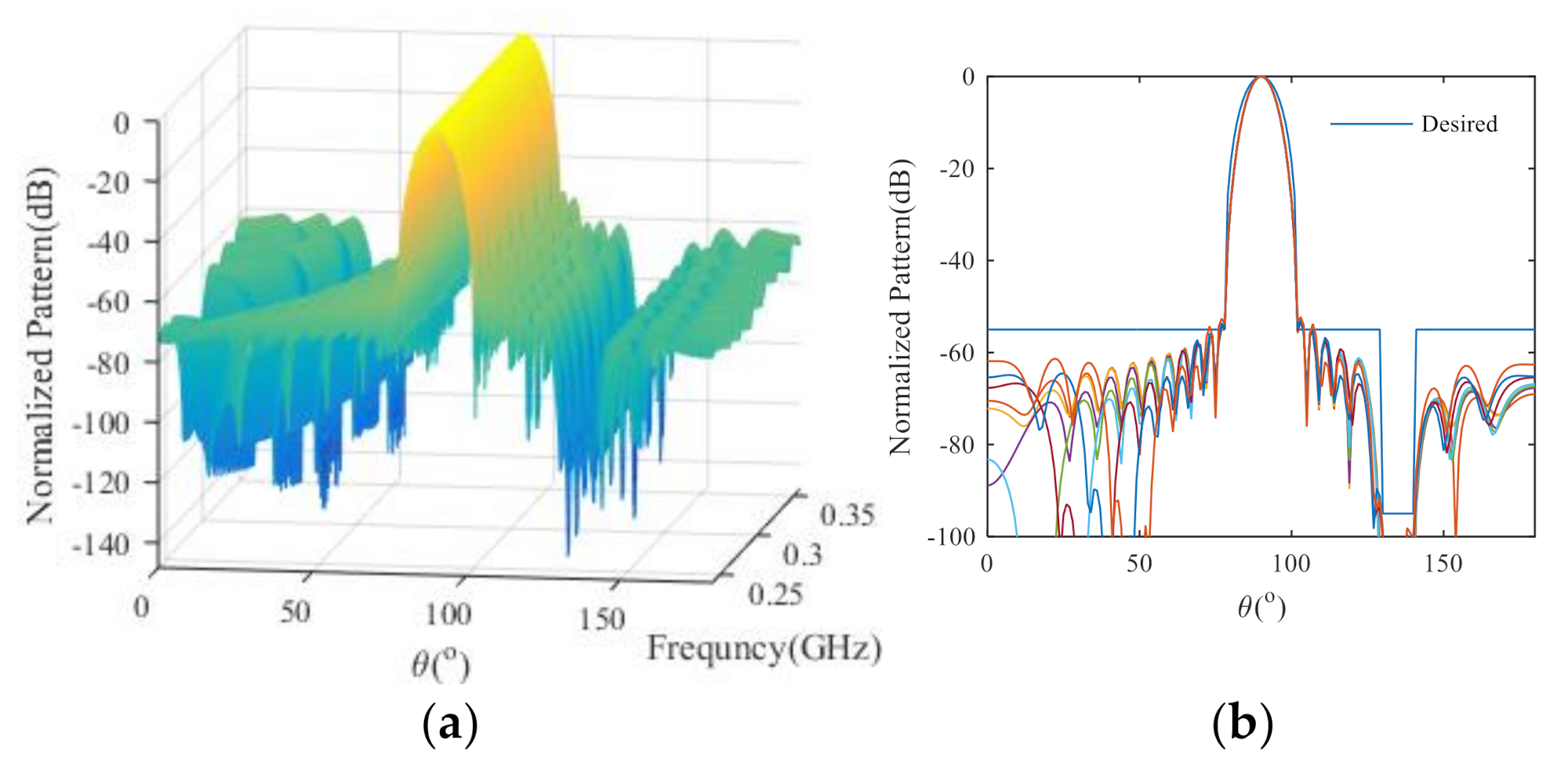
A 23-element uniform linear array with FI pattern is synthesized by the algorithm proposed in this paper. Eight sub arrays are used to realize the wideband frequency invariance of the pattern. Elapsed time is 0.071521 s. Figure 4a shows the spatial and frequency domain pattern of the array. The desired pattern and the pattern of the center frequency of each sub array F_i in the bandwidth of sub array are shown in Figure 4b. It can be seen that the main lobe of the array has a good frequency invariant property in broadband. Compared with the reference [23], the SLL of the FI array realized in this paper is 15 dB lower.

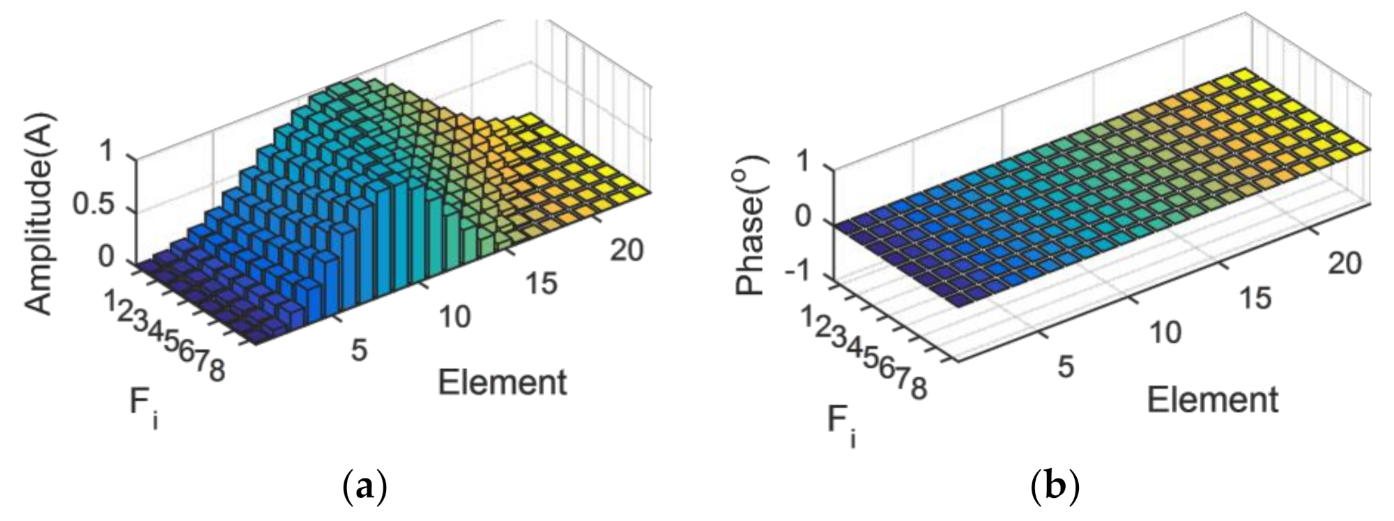
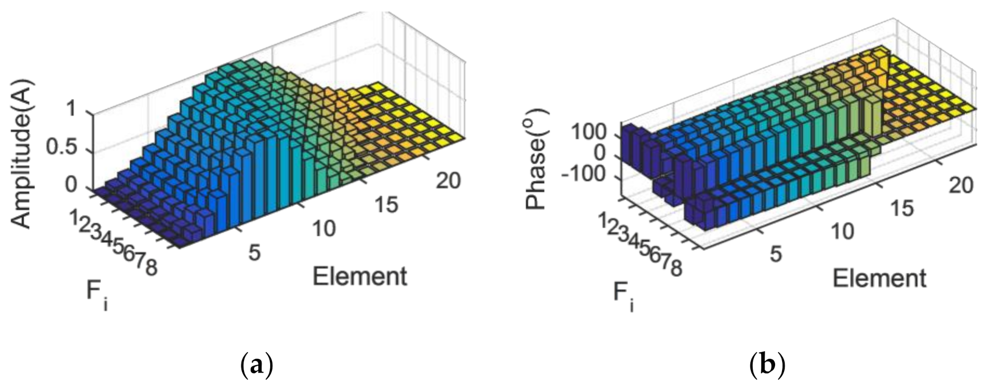
Figure 5 shows the amplitude and phase of the array excitation matrix W. W is a matrix of N × M dimensions. The element ${\omega }_{nl}$ in matrix W is shown in the Figure 1, which represents the excitation of the nth element in the sub array F_l. It can be seen from Figure 5 that the amplitude of array excitation is a taper distribution with the same phase.

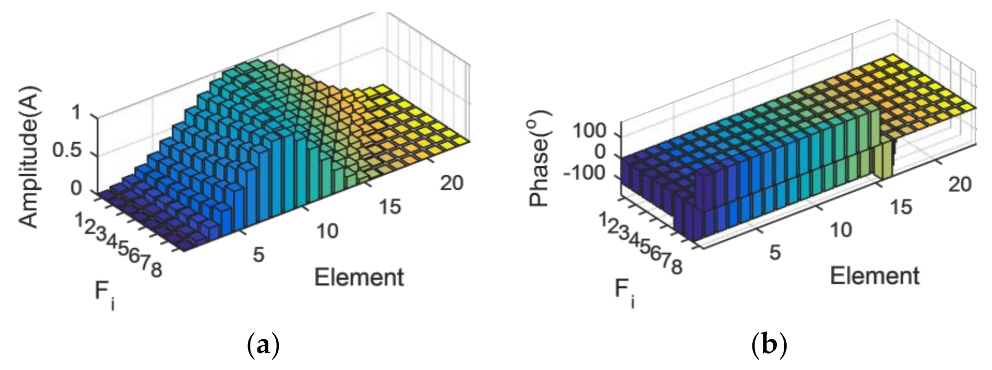
A reduction in the number of elements is very important to reduce the array complexity. In this paper, the number of elements in the array is further reduced to 18. As shown in Figure 6, the SLL of the array is −40 dB. Compared with the reference [23], the number of elements is reduced by 21.7%, and the SLL is at the same level. Only six sub arrays are needed to achieve the wideband FI. As can be seen from Figure 7, when the array element is reduced, the excitation phase of the FI array element is no longer uniform. The algorithm running time is 0.062391 s. Computing time was further reduced by 12.8%.

In order to quantify the change of beam width with frequency,

Table 2. The HPBW variation of the array pattern in the bandwidth.

Element Number	Maximum(°)	Minimum(°)	Mean(°)
18	8.7	8.1	8.3
23	7.5	7.1	7.3

shows the change data of HPBW in the bandwidth. It can be seen that the FI array synthesized by the algorithm has good beam stability. With the increase in the number of array elements, the beam stability is improved.

In this case, the synthesis effect of the algorithm for asymmetric pattern is also verified. There is a −95 dB notch at (130°–140°). The simulation time of this example is 0.078176 s. Compared with the example in the reference [23], the notch depression in Figure 8 is 45 dB lower. Figure 9 shows the results of the array excitation matrix. When the pattern is asymmetric, the excitation phases of individual array elements are not consistent. It can be seen that the algorithm proposed in this paper can control the array pattern in the wide band.

3.2. Uniform Linear Array of 64 Isotropic Ideal Point Elements

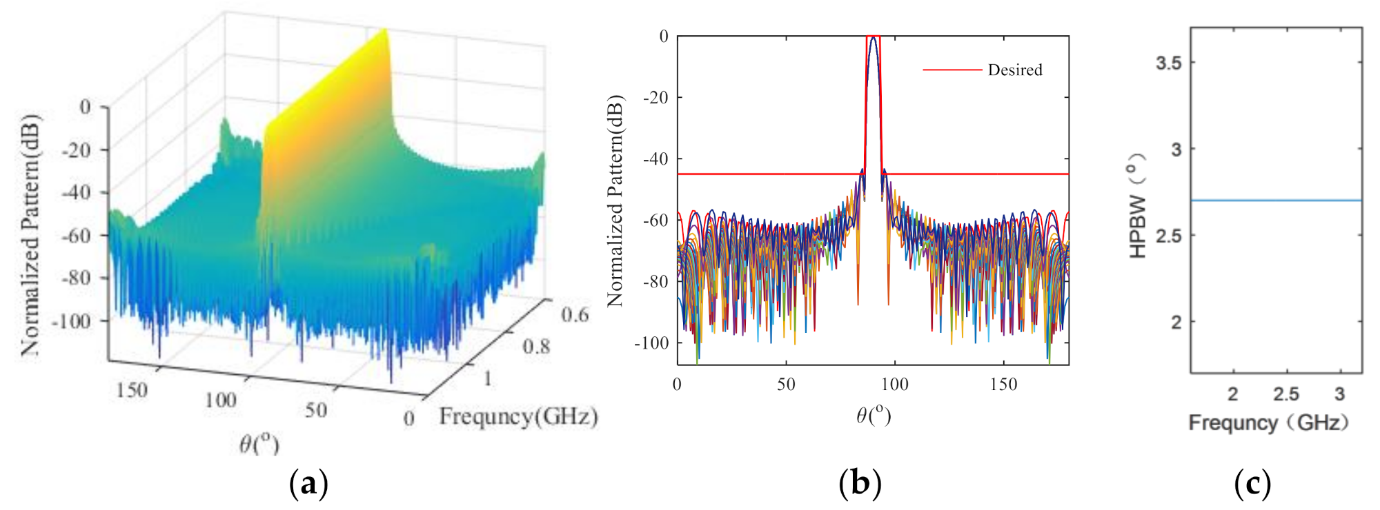
In this case, a 64-element pen beam FI array is synthesized. The array worked in the frequency band (0.6–1.2 GHz). The array element spacing is 0.45${\lambda }_{\max }$. ${\lambda }_{\max }$ is the wavelength corresponding to frequency 0.6 GHz. Using the algorithm proposed in this paper, a wide-band FI array is synthesized with 32 subarrays. Elapsed time is 0.515945 s. The results in Figure 10b show that the SLL of the array is lower than −40 dB, which is 20 dB lower than the results in the reference [21].

As can be seen from Figure 10c, the HPBW of the array pattern is stable at 2.7° in the whole bandwidth range. It can be seen from Figure 11 that the number of elements used in the subarray is gradually decreasing with the increase in frequency. The subarray at the highest frequency uses almost half of the elements of the low frequency subarray.

3.3. Uniform Linear Array of 44 Isotropic Ideal Point Elements

This example further verifies the effectiveness of the algorithm for non-symmetrical FI array synthesis. In this example, a 44-element uniformly spaced linear array working at (0.5–1 GHz) is synthesized [22]. The main lobe of the array pattern points to 100 degrees. In the algorithm proposed, the spacing of the elements in the array is 0.39${\lambda }_{\max }$, which is 0.11${\lambda }_{\max }$ in the reference [22]. It can be seen that the FI array synthesized by the algorithm in this paper is easier to be realized. In this case, 22 FI sub arrays are used. Figure 12 shows the pattern of the array. In the bandwidth range, the mean value of HPBW is 4.339 degrees, and the variation range is less than 0.3 degrees. The SLL of the array is less than −35 dB, which is 5 dB lower than the value in the reference [22]. As shown in Figure 13, in order to scan the array pattern to 10 degrees, the excited phase of the array elements must be modulated.

3.4. Uniform Linear Array with Isotropic Antennas

In the application of the wideband array, the wideband antenna plays an important role. Most of the references and the three examples mentioned above use isotropic ideal point source as the array element to verify the performance of the FI array synthesis algorithm. In practical engineering, the mutual coupling between the elements will lead to an inconsistency in the element pattern and increase the difficulty of the FI array synthesis. In this case, a broadband antenna will be designed. Using the antenna to form a broadband array, the effectiveness of the proposed FI array synthesis algorithm is verified. The active patterns (AP) of elements and the patterns of arrays are obtained by HFSS 19.2.

There are many studies about the design of broadband antenna, and about 40% of the bandwidth is achieved when the SWR is less than two. The bandwidth of the antenna cannot meet the bandwidth requirements of the broadband FI array. Moreover, the antenna gain varies widely in the bandwidth, which is not suitable for broadband communication. Kwai-Man Luk et al. proposed a broadband antenna structure based on the equivalent electric dipole and magnetic dipole model [27]. The widest bandwidth of the antenna is 71% (SWR < 2), and the gain variation in the band is less than 1 dB.

In this paper, the antenna feed strip is redesigned with a bent structure. A new slot has been made in the antenna arm. HFSS 19.2 is used to simulate the antenna with the structure shown in Figure 14. Figure 16 shows the results of full wave simulation analysis with software. With the introduction of the new structure, the bandwidth of the antenna increases to 108% for S₁₁ < −10 dB (1.55–3.22 GHz). As shown in Figure 15b, the antenna gain is stable at 7.96 dB and the variation range is 0.42 dB. It can be seen from Figure 16 that the antenna is an omnidirectional antenna and a broadband FI antenna.

In this paper, a 23-element uniform linear array is first formed along the y-axis with a spacing of 93.8 mm (0.5λ @ 1.6 GHz). The frequency band of the FI array is (1.6–2.4 GHz). The desired SLL of the FI array is lower than −40 dB. The main lobe of array pattern satisfies ${\cos }^2\left[7\left(\theta +\frac{\pi }{2}\right)\right]$. The array structure is shown in Figure 17. It can be seen from the above algorithm that 8 sub arrays are needed to realize the FI array. HFSS 19.2 is used to simulate the FI array at the center frequency of 8 sub arrays. The AP $p_{mn}(f_{l0},{\theta }_m)$ of each element at the center frequency of each sub array is extracted. Bringing the AP of all elements into Equation (2) obtains the matrix P. The excitation vector $w_l$ of each sub array is obtained by the algorithm flow described in Figure 3. By introducing $w_l$ into HFSS, the pattern of the sub array can be obtained. Repeat this process to obtain the excitation vectors of all sub arrays and the pattern of the FI array in the frequency band as shown in Figure 18.

The simulation results show that the FI array synthesized by this algorithm can achieve frequency invariant pattern in the bandwidth. Compared with the result in Section 3.1, the SLL of the array is 15 dB higher due to the mutual coupling of the elements. Additionally, the elements in the array are no longer fed by the same phases, as shown in Figure 19. The mean value of HPBW in the bandwidth is 7.4 degrees, and the variation range is 0.2 degrees.

Furthermore, this paper synthesizes a 64-element FI array working at (1.6–3.2 GHz). A total of 32 subarrays are used to ensure the stability of the main lobe in the whole bandwidth.

As can be seen from Figure 20, the peak SLL of the array pattern is −45.12 dB. Furthermore, Figure 20 also shows that the HPBW of the 64-element FI array in this example is always 2.7 degrees in the bandwidth. This result is consistent with Figure 10. Figure 21 shows the excitation matrix of the array in this example. Compared with the excitation matrix of the isotropic ideal point element in Section 3.2, the excitations of the elements in this case are no longer the same as the excitations of the last example due to the difference between the active patterns of the elements.

4. Discussion

In this paper, an analytic method of FI array synthesis is proposed by SVD. The uniform linear array with low frequency as reference is the common array aperture of the whole broadband.

In order to verify the effectiveness of the algorithm, the FI array composed of isotropic ideal point elements or broadband antenna elements is synthesized. In this paper, the synthesis results of five FI arrays with isotropic ideal point elements are compared. The simulation results are listed in

Table 3. The conclusion of simulation results.

Pattern	${\mathbf{cos}}^2\left[7\left(\mathit{\theta }+\frac{\mathit{\pi }}{2}\right)\right]$	${\mathbf{cos}}^2\left[7\left(\mathit{\theta }+\frac{\mathit{\pi }}{2}\right)\right]$	${\mathbf{cos}}^2\left[7\left(\mathit{\theta }+\frac{\mathit{\pi }}{2}\right)\right]\mathbf{with}\mathbf{Notch}$	Pencil Beam	Scanning Beam
Reference	[23]	[23]	[23]	[21]	[22]
Number in reference	23	23	23	64	44
Number in paper	23	18	23	64	44
SLL in reference (dB)	−40	−40	−40	−20	−30
SLL in paper (dB)	−55	−40	−55	−42	−35
Notch in reference (dB)			−50
Notch in paper (dB)			−95

. With the same number of elements, the SLL of the array in this paper can be lower than that in the reference. Under the same SLL constraint, the number of array elements in this paper is less. The research of the array synthesis algorithm which can contain the difference of radiation patterns of array elements in the actual array is the focus of FI array synthesis.

According to the active wideband pattern of elements in the array, two wideband FI arrays are synthesized. Finally, the results of the array synthesis are verified by full wave simulation. The simulation results show that the algorithm can synthesize the FI array quickly and effectively.

5. Conclusions

An analytic method of FI array synthesis is proposed and verified in this paper. The number of elements in FI array is reduced to 78.3%.In order to further reduce the number of elements and increase the bandwidth of the FI array, it needs to be designed based on the research of a non-uniformly spaced FI array.