Improved Salp Swarm Optimization Algorithm: Application in Feature Weighting for Blind Modulation Identification

Abstract

In modulation identification issues, like in any other classification problem, the performance of the classification task is significantly impacted by the feature characteristics. Feature weighting boosts the performance of machine learning algorithms, particularly the class of instance-based learning algorithms such as the Minimum Distance (MD) classifier, in which the distance measure is highly sensitive to the magnitude of features. In this paper, we propose an improved version of the Salp Swarm optimization Algorithm (SSA), called ISSA, that will be applied to optimize feature weights for an MD classifier. The aim is to improve the performance of a blind digital modulation detection approach in the context of multiple-antenna systems. The improvements introduced to SSA mainly rely on the opposition-based learning technique. Computer simulations show that the ISSA outperforms the SSA as well as the algorithms that derive from it. The ISSA also exhibits the best performance once it is applied for feature weighting in the above context.

1. Introduction

Feature weighting is a crucial preprocessing step before creating a machine learning (ML) model. It is a technique employed to estimate the optimal degree of influence of features, individually, using a training set. When well-weighted, high weights are attributed to important features while lower weights are attributed to irrelevant and noisy features, i.e., features that likely deteriorate the accuracy of the ML model [1,2]. In literature, there is a lack of investigation of the performance of metaheuristic optimization algorithms in feature weighting.

Due to the good performance shown in a wide range of real-world optimization problems, including in ML [3,4,5], metaheuristic algorithms seem to be good candidates to be deployed for dataset preprocessing techniques, such as feature weighting. There are three basic categories of these algorithms: physics-based [6], evolutionary-based [7], and swarm-based [8]. The Salp Swarm Algorithm (SSA) is a recently swarm-based optimization algorithm which was proposed by Mirjalili and al. [9]. In this paper, we propose an improved version of the SSA, referred to as Improved Salp Swarm Algorithm (ISSA), that later on will be utilized for weighting features.

The main contributions of this paper are four-fold: (i) a weight factor is introduced in the position update formula of the SSA. This factor varies dynamically to balance the ability of exploration and exploitation; (ii) a control parameter is added to the whole search process of the SSA (instead of the initialization only) to improve the accuracy of the solution; (iii) to overcome premature convergence of SSA and evolution stagnation, an Opposition Based Learning technique (OBL) is employed during the search process; and (iv) the improved optimization algorithm is applied for a feature weighting example in such a way that it gives a better misclassification rate for the studied classification problem. The classification problem that we considered in this paper is the blind digital modulation identification (DMI) for multiple-antenna systems.

Although several trials have been made to improve SSA’s performance, they are still suffering from the problem of stagnation at local minima in some cases. To highlight its effectiveness, the ISSA is compared first with the original SSA as well as two algorithms that derive from it: Space Transformation SSA (STSSA) [10], which uses space transformation search, and Inertia Weight SSA (IWSSA) [11], in which an inertia weight is embedded.

The rest of the paper is organized as follows. In Section 2, we formulate the optimization problem. Section 3 presents a description of the original SSA and introduces our motivation and improvements. Section 4 gives an overview on the comparison methodology and the materials used. In Section 5, the proposed algorithm is evaluated by sixteen optimization benchmark functions. The performance of the ISSA in feature weighting is discussed in Section 6. Finally, Section 7 summarizes the main findings of this study and suggests directions for future research.

2. Problem Formulation

To show its scalability for real-world applications, the ISSA is applied for feature weighting in the context of blind digital modulation recognition for a multi-antenna system. The signals model and the identification system are the ones employed in [12]. The system model considers a frequency-flat block-fading multiple-input–multiple-output (MIMO) channel with m transmitting antennas and n receiving antennas. The identification process is based on one of the most popular strategies used for the blind DMI issue in MIMO systems [13,14]. The identification is three-staged: (i) the blind source separation stage is first, (ii) feature extraction for each one of the separated streams takes place, and (iii) the modulation scheme for each separated stream is identified through the minimum distance (MD) classifier. The extracted features used to estimate the modulation type on separated streams are the Higher-Order Statistics (HOS). The MD classifier identifies the modulation scheme by calculating the Euclidean distance of a feature vector with all the theoretical ones and then selecting the closest. In order to improve the performance of the identification system, authors in [12] introduced a feature-denoising approach. In our paper, for the same purpose, we will embed a feature weighting approach, i.e., we added weights to the initially extracted HOS so that the misclassification rate is minimized. Therefore, the optimization problem can be formulated as follows:

$$\begin{array}{cc}\hfill {\mathit{\alpha }}^{*}& =\underset{\mathit{\alpha }\in {\mathbb{R}}^{(1\times \mathsf{nf})+}}{\arg \min }\frac{1}{\left|\mathcal{S}\right|}\sum _{i\in \mathcal{S}}〚({\varphi }_j|\underset{j\in \{1\cdots |\varphi \left|\right\}}{\arg \min }\left|\right|\mathit{\alpha }\odot {\mathbf{s}}_i-{\mathbf{v}}_j\left|\right|)\ne {\phi }_i〛,\hfill \end{array}$$

(1)

where $\mathit{\alpha }$ is the weighting vector, the Iverson bracket $〚.〛$ is a function that takes a truth value inside and returns 1 or 0 accordingly, $|.|$ denotes the cardinality of the dataset $\mathcal{S}$, and $\left|\right|.\left|\right|$ indicates the Euclidean norm of a vector. ${\mathbf{s}}_i\in {\mathbb{R}}^{1\times \mathsf{nf}}$ represents the vector of $\mathsf{nf}$ features. $\varphi$ is the set of possible modulation schemes. The expression inside the big parentheses returns the ith estimated modulation type that corresponds to the feature vector ${\mathbf{s}}_i$ (i.e., a vector of estimated HOS). ${\mathbf{v}}_j$ is the theoretical HOS vector for the modulation ${\varphi }_j$ and ${\phi }_i$ is the true modulation scheme for the sample i of the dataset (i.e., the ith estimated HOS vector). ⊙ denotes component-wise multiplication.

3. Improvements on Salp Swarm Algorithm

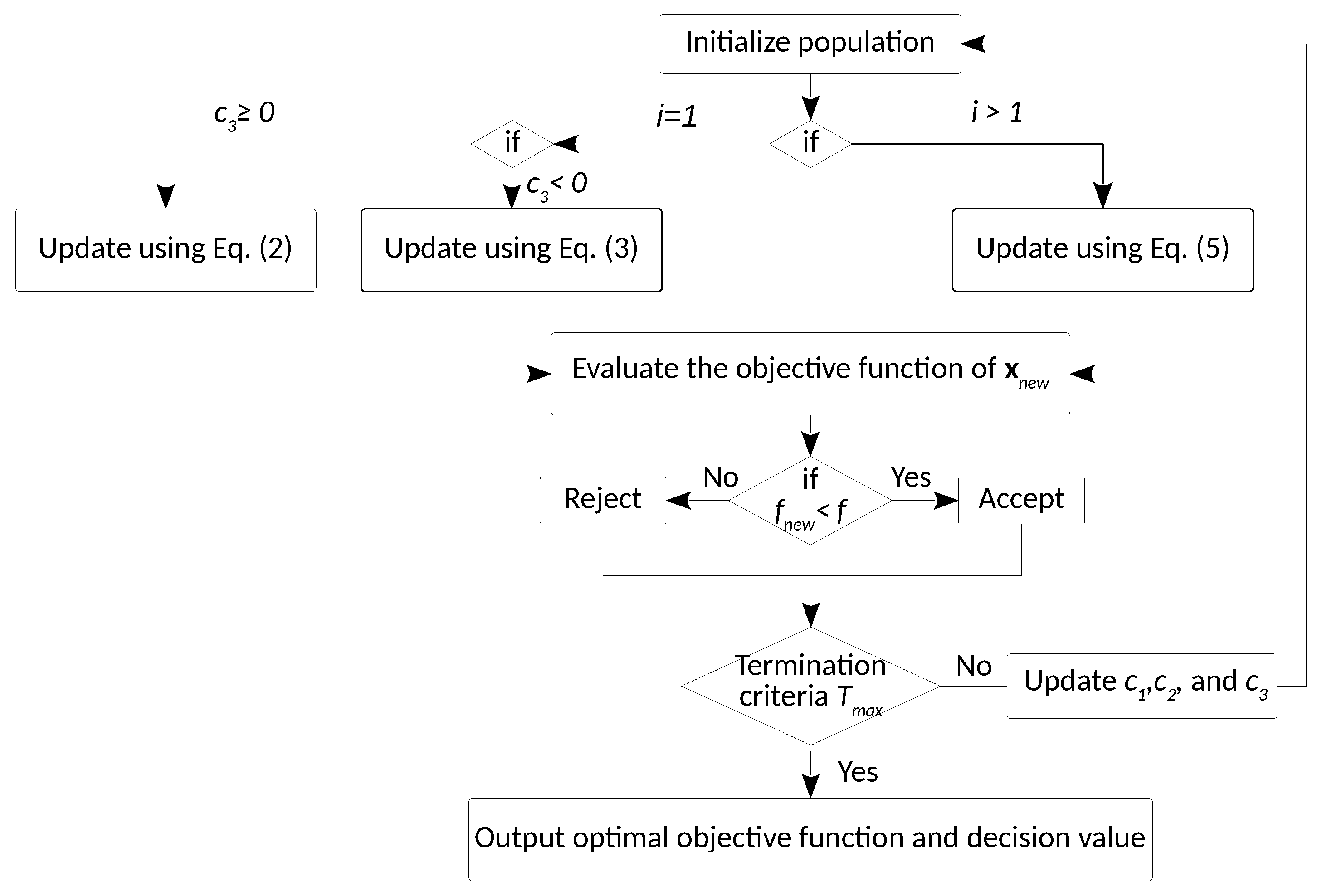
3.1. SSA, the Basic Algorithm

SSA simulates the swarming mechanism of salps when they are hunting arround oceans. In massive oceans, salps usually shape a swarm identified as a salp chain. In the SSA, the leader is the salp at the front of the chain, and the rest of the salps are called followers. Equation (2) updates the leader’s position for the iteration $k+1$:

$${\mathbf{x}}_i^1[k+1]=\left\{\begin{array}{cc}{\mathbf{f}}_i\left[k\right]+c_1\left(\left({\mathbf{u}}_i-{\mathbf{l}}_i\right)c_2+{\mathbf{l}}_i\right)& c_3\ge 0,\\ {\mathbf{f}}_i\left[k\right]-c_1\left(\left({\mathbf{u}}_i-{\mathbf{l}}_i\right)c_2+{\mathbf{l}}_i\right)& c_3<0,\end{array}\right.$$

(2)

where ${\mathbf{x}}_i^1$ presents the position of the first salp (leader) in the ith dimension, ${\mathbf{f}}_i$ is the position of the food source in the ith dimension. ${\mathbf{u}}_i$ and ${\mathbf{l}}_i$ indicate the upper and the lower bounds of ith dimension, respectively. $c_2$ and $c_3$ are random numbers generated in $[0,1]$. The coefficient $c_1$ is the most critical parameter in SSA because it balances exploration and exploitation and it is defined as follows:

$$c_1=2\exp \left(-{\left(\frac{4k}{T_{max}}\right)}^2\right),$$

(3)

where k is the current iteration, and $T_{max}$ represents the maximum number of iterations. Equation (4) updates the position of the followers for the iteration $k+1$:

$$\begin{array}{cc}\hfill {\mathbf{x}}_i^j[k+1]& =\frac{1}{2}\left({\mathbf{x}}_i^j\left[k\right]+{\mathbf{x}}_i^{j-1}\left[k\right]\right),\hfill \end{array}$$

(4)

where $j\ge 2$, ${\mathbf{x}}_i^j$ is jth follower’s salp position in ith dimension and ${\mathbf{x}}_i^{j-1}$ is the $(j-1)$th follower’s salp position in ith dimension.

It is worth noting that the dimension of all vectors described above is the number of objective function variables. Figure 1 illustrates the flowchart of the SSA. f presents the best fitness getting from the previous iterations. The subscript new refers to the values of the current iteration.

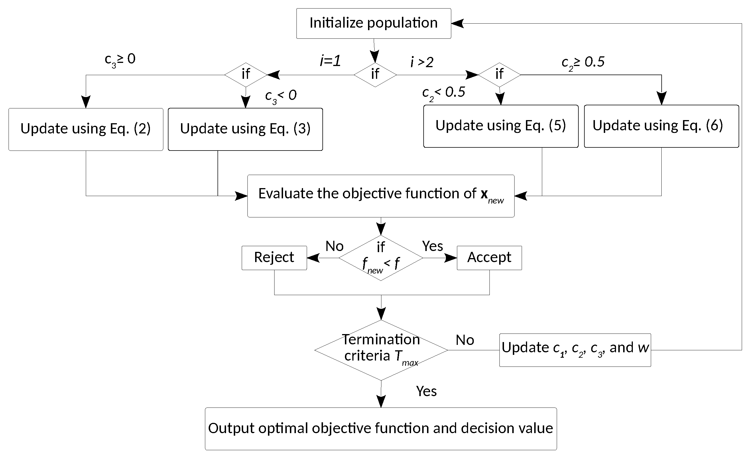
3.2. Motivation and Improvements

SSA stores the best solution in the food source variable. Thus, it is very competitive in exploiting search space. Like many other optimization algorithms, SSA is still suffering from the problem of local stagnation and low convergence speed. Figure 2a and Figure 3a show the evaluated solutions using the SSA for optimizing $f_3$ and $f_4$ (two selected benchmark functions [9]), respectively. Their correspondent convergence visualizations are plotted in Figure 2b and Figure 3b, respectively. As shown in these figures, the algorithm fails in reaching the best solution (i.e., the $(0,0)$ pair). Besides, we can affirm the powerlessness of SSA in converging to the global optima.

To overcome these drawbacks, we propose an improved SSA called ISSA. The main improvements in the ISSA are as follows. Firstly, an inertia weight $w\in [0,1]$ is introduced into SSA. This parameter accelerates the convergence speed during the search. It also makes a balance between exploitation and exploration capabilities to escape local solutions. Secondly, the performance of the ISSA is highly influenced by $c_1$. In fact, $c_1$ is decreased by exploring and exploiting the search space, which achieves a precise appreciation of the optimal solution. The new update formula is displayed in (5):

$$\begin{array}{cc}\hfill {\mathbf{x}}_i^j[k+1]& =w\frac{1}{2}\left({\mathbf{x}}_i^j\left[k\right]+c_1{\mathbf{x}}_i^{j-1}\left[k\right]\right).\hfill \end{array}$$

(5)

Finally, the convergence rate of the algorithm is not stable and will be slow in most cases. Therefore, we apply the OBL technique [15,16]. This technique can bring the algorithm closer to the global optima, creating more flexibility in exploring search space and quickly converging towards an optimal value. Mathematically, OBL can be represented as in (6):

$$\begin{array}{cc}\hfill {\mathbf{x}}_i^j[k+1]& =\left({\mathbf{u}}_i-{\mathbf{l}}_i\right)+w{c}_1{\mathbf{x}}_i^j\left[k\right].\hfill \end{array}$$

(6)

Figure 2c and Figure 3c show the evaluated solutions using the ISSA for optimizing $f_3$ and $f_4$, respectively. Their correspondent convergence visualizations are illustrated in Figure 2d and Figure 3d, respectively. As can be observed from these figures, the ISSA succeeds in achieving a satisfactory level in attending to the best solution. Moreover, it converges faster toward global optima. All the above results confirm that these improvements enhance the SSA. Figure 4 illustrates the flowchart of the SSA.

4. Comparison Methodology and MATERIALS

4.1. Comparison Methodology

In literature, there are many metaheuristic optimization algorithms and trials of improvements of the SSA. As mentioned in the Introduction, many of them still suffer from some weaknesses, mainly the inability to stay away from local minima. For the rest of them, our choice for the benchmarking algorithms is based on the following criteria. The original version of the algorithm (SSA) and some recent improvements in the closest context for the application. Since there is no work on feature weighting as yet, the closest context of application is generally machine learning related and specifically feature selection. Consequently, we selected STSSA and IWSSA as trials of improvements of the SSA for comparison.

In order to have a complete comparison, i.e., a comparison that is not limited only to the application (e.g., feature selection in the context of this paper), the ISSA should first exhibit a good performance once tested on a set of mathematical functions (functions that are usually used to evaluate a metaheuristic optimization algorithm). In fact, a good optimization algorithm should not be tailored to a specific function or application; for that reason, we first evaluated the designed optimization algorithm on a wide and diversified set of benchmark functions, i.e., unimodal functions (one local minimum, configurable number of spatial dimensions), multimodal functions (many local minima, configurable number of spatial dimensions), and fixed-dimension multimodal functions (many local minima, fixed number of spatial dimensions). This study is conducted on both accuracy and convergence speed, and forms the content of Section 5.

The comparison within the application context is carried out once the algorithm shows fine performance against other algorithms used for comparison. Therefore, in Section 6, we assess the performance of the ISSA in opposition to other optimization algorithms in the context of features weighting.

4.2. Materials

For all computer simulations of this paper, we used Matlab version 9.9.0.1538559 (R2020b) Update 3. To replicate and build on the results, the source code for this work is available since 7 August 2021, on https://github.com/sofiane-kharbech/Feature-Weighting-for-DMI under the MIT license.

5. Benchmarking of SSA and ISSA

The performance of the proposed ISSA is tested by solving 16 benchmark functions under dimension 30 (dimension of agent) reported in [17]. These functions are grouped into unimodal functions ($f_1-f_7$) with one local optimum, multimodal functions ($f_8-f_{13}$) with a lot of local optima, and fixed-dimension multimodal functions ($f_{14}-f_{16}$). For all tests, the number of search agents is set to 40. In addition to the original SSA, the proposed ISSA is compared with two other improvements on SSA, STSSA [10], and IWSSA [11].

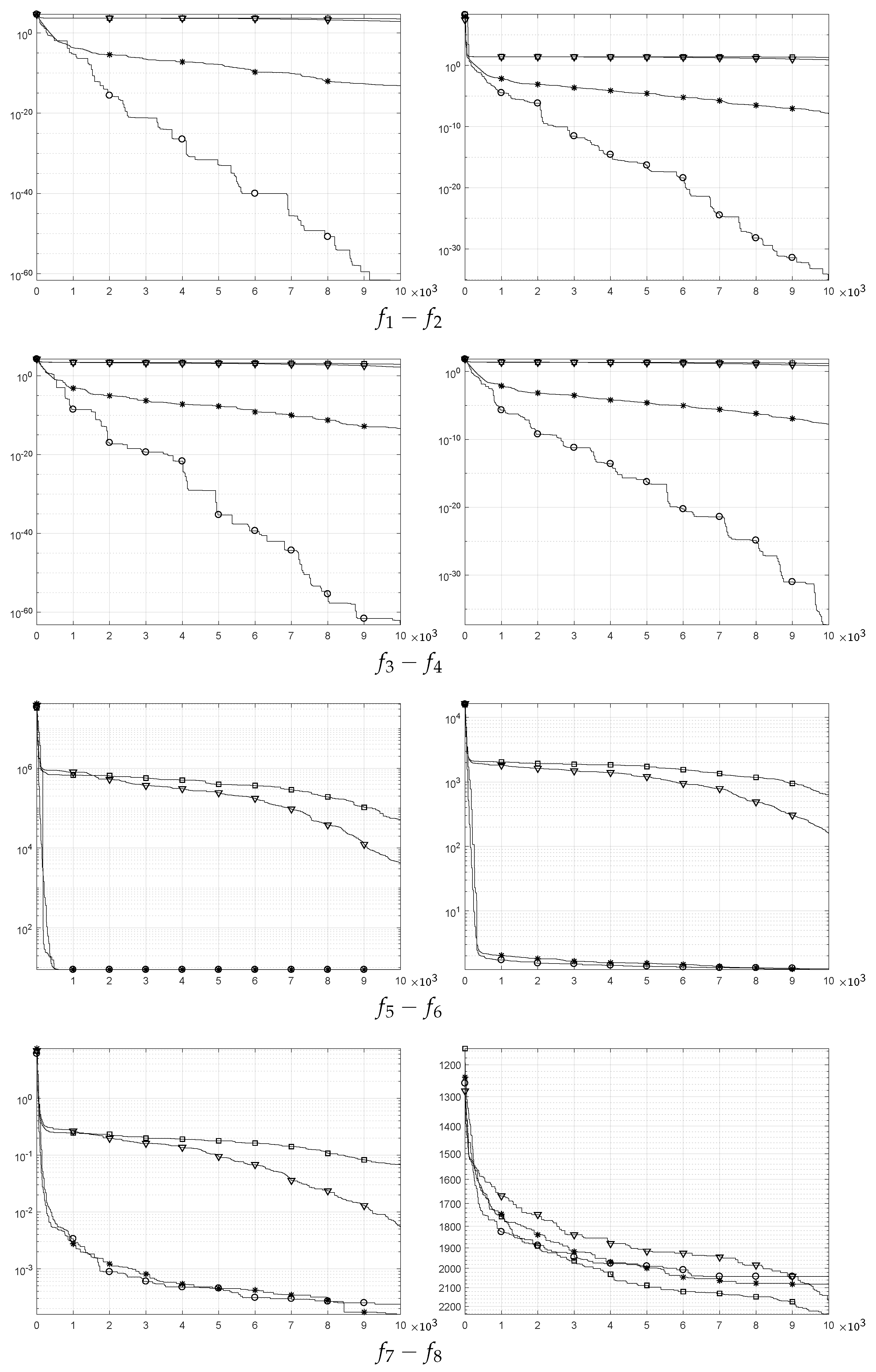
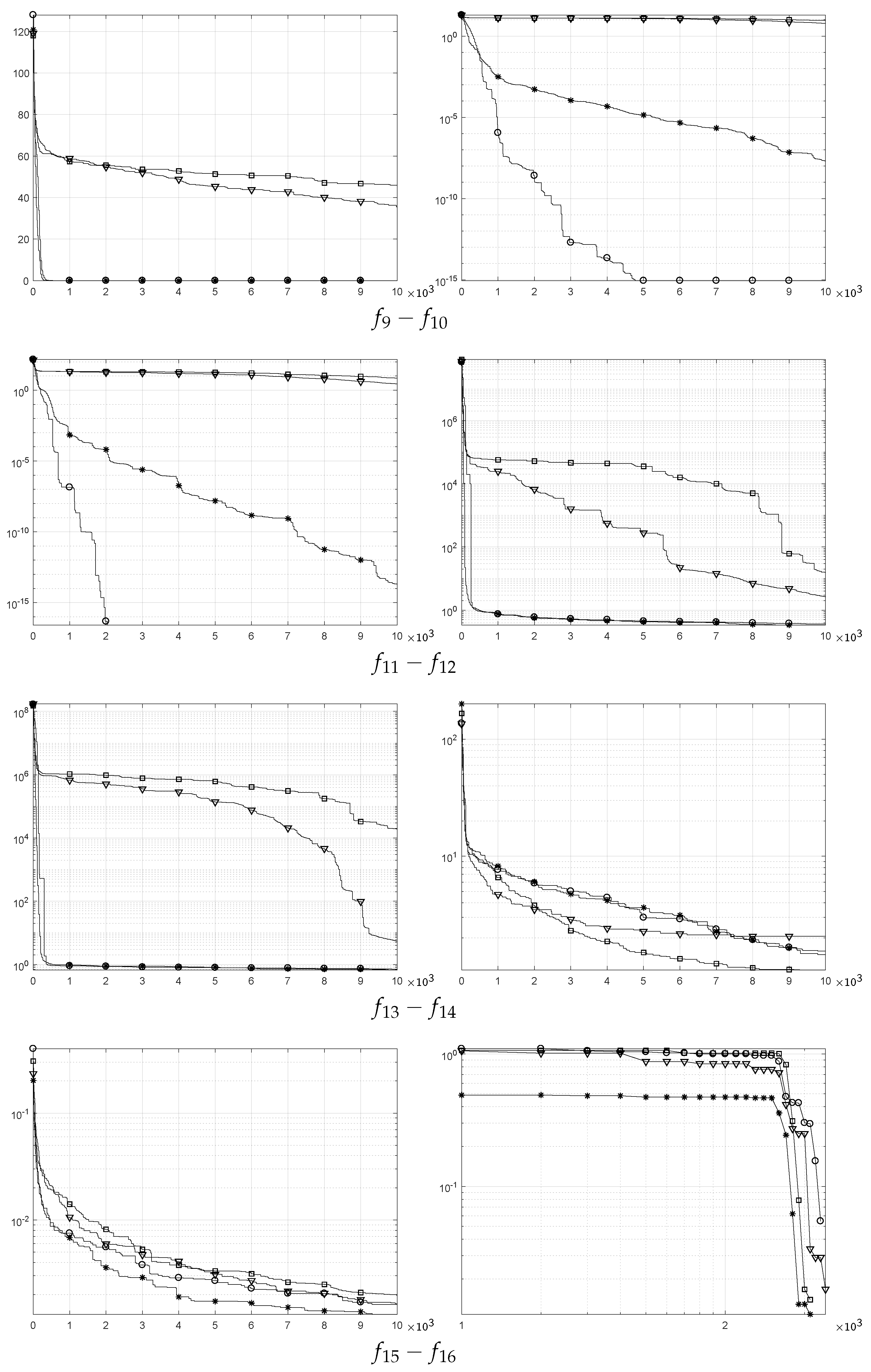
5.1. Comparison Based on Solution Accuracy

Table 1. Mean, SEM, and SD for functions $f_1-f_{16}$ obtained by SSA, STSSA, IWSSA, and ISSA.

		SSA	STSSA	IWSSA	ISSA
$f_1$	Mean	4.03 × 10${}^{-9}$	7.12 × 10${}^{-10}$	1.01 × 10${}^{-23}$	0.00 × 10${}^{\mathbf{0}}$
	SD	9.52 × 10${}^{-10}$	2.78 × 10${}^{-10}$	3.48 × 10${}^{-23}$	0.00 × 10${}^{\mathbf{0}}$
	SEM	1.73 × 10${}^{-10}$	5.08 × 10${}^{-11}$	6.35 × 10${}^{-24}$	0.00 × 10${}^{\mathbf{0}}$
$f_2$	Mean	1.90 × 10${}^{-1}$	8.90 × 10${}^{-6}$	9.00 × 10${}^{-13}$	1.20 × 10${}^{-\mathbf{180}}$
	SD	7.10 × 10${}^{-1}$	1.54 × 10${}^{-6}$	1.17 × 10${}^{-12}$	0.00 × 10${}^{\mathbf{0}}$
	SEM	1.20 × 10${}^{-1}$	2.82 × 10${}^{-7}$	2.13 × 10${}^{-13}$	0.00 × 10${}^{\mathbf{0}}$
$f_3$	Mean	1.93 × 10${}^{-9}$	2.20 × 10${}^{-10}$	1.78 × 10${}^{-23}$	0.00 × 10${}^{\mathbf{0}}$
	SD	1.01 × 10${}^{-9}$	1.24 × 10${}^{-10}$	3.61 × 10${}^{-23}$	0.00 × 10${}^{\mathbf{0}}$
	SEM	1.84 × 10${}^{-10}$	2.28 × 10${}^{-11}$	6.60 × 10${}^{-24}$	0.00 × 10${}^{\mathbf{0}}$
$f_4$	Mean	1.50 × 10${}^{-5}$	7.73 × 10${}^{-6}$	9.02 × 10${}^{-13}$	2.27 × 10${}^{-\mathbf{172}}$
	SD	4.17 × 10${}^{-6}$	1.78 × 10${}^{-6}$	9.66 × 10${}^{-13}$	0.00 × 10${}^{\mathbf{0}}$
	SEM	7.63 × 10${}^{-7}$	7.63 × 10${}^{-7}$	1.76 × 10${}^{-13}$	0.00 × 10${}^{\mathbf{0}}$
$f_5$	Mean	1.40 × 10${}^2$	89.4 × 10${}^{-1}$	89.2 × 10${}^{-\mathbf{1}}$	89.2 × 10${}^{-\mathbf{1}}$
	SD	3.59 × 10${}^2$	1.60 × 10${}^{-2}$	1.40 × 10${}^{-\mathbf{2}}$	1.20 × 10${}^{-\mathbf{2}}$
	SEM	6.56 × 10${}^1$	0.3 × 10${}^{-2}$	0.2 × 10${}^{-\mathbf{2}}$	0.2 × 10${}^{-\mathbf{2}}$
$f_6$	Mean	6.31 × 10${}^{-\mathbf{10}}$	0.13 × 10${}^1$	6.00 × 10${}^{-1}$	6.30 × 10${}^{-1}$
	SD	2.72 × 10${}^{-\mathbf{10}}$	3.30 × 10${}^{-1}$	1.40 × 10${}^{-1}$	1.70 × 10${}^{-1}$
	SEM	4.98 × 10${}^{-\mathbf{11}}$	0.60 × 10${}^{-1}$	0.20 × 10${}^{-1}$	0.30 × 10${}^{-1}$
$f_7$	Mean	0.60 × 10${}^{-2}$	8.19 × 10${}^{-5}$	4.44 × 10${}^{-\mathbf{5}}$	4.69 × 10${}^{-5}$
	SD	0.40 × 10${}^{-2}$	8.38 × 10${}^{-5}$	4.16 × 10${}^{-\mathbf{5}}$	4.58 × 10${}^{-5}$
	SEM	0.40 × 10${}^{-3}$	1.53 × 10${}^{-5}$	7.60 × 10${}^{-\mathbf{6}}$	8.37 × 10${}^{-6}$
$f_8$	Mean	−2.83 × 10${}^3$	−2.23 × 10${}^3$	−2.093 × 10${}^{\mathbf{3}}$	−2.096 × 10${}^3$
	SD	2.54 × 10${}^2$	1.91 × 10${}^2$	1.54 × 10${}^{\mathbf{2}}$	1.65 × 10${}^2$
	SEM	4.65 × 10${}^1$	3.50 × 10${}^1$	2.82 × 10${}^{\mathbf{1}}$	3.01 × 10${}^1$
$f_9$	Mean	1.94 × 10${}^1$	1.01 × 10${}^{-10}$	0.00 × 10${}^{\mathbf{0}}$	0.00 × 10${}^{\mathbf{0}}$
	SD	0.75 × 10${}^1$	3.62 × 10${}^{-11}$	0.00 × 10${}^{\mathbf{0}}$	0.00 × 10${}^{\mathbf{0}}$
	SEM	0.13 × 10${}^1$	6.61 × 10${}^{-12}$	0.00 × 10${}^{\mathbf{0}}$	0.00 × 10${}^{\mathbf{0}}$
$f_{10}$	Mean	7.50 × 10${}^{-1}$	6.17 × 10${}^{-6}$	6.11 × 10${}^{-13}$	8.88 × 10${}^{-\mathbf{16}}$
	SD	8.10 × 10${}^{-1}$	1.57 × 10${}^{-6}$	8.03 × 10${}^{-13}$	0.00 × 10${}^{\mathbf{0}}$
	SEM	1.40 × 10${}^{-1}$	2.87 × 10${}^{-7}$	1.46 × 10${}^{-13}$	0.00 × 10${}^{\mathbf{0}}$
$f_{11}$	Mean	2.60 × 10${}^{-1}$	9.36 × 10${}^{-10}$	0.00 × 10${}^{\mathbf{0}}$	0.00 × 10${}^{\mathbf{0}}$
	SD	1.40 × 10${}^{-1}$	4.36 × 10${}^{-10}$	0.00 × 10${}^{\mathbf{0}}$	0.00 × 10${}^{\mathbf{0}}$
	SEM	0.20 × 10${}^{-1}$	7.97 × 10${}^{-11}$	0.00 × 10${}^{\mathbf{0}}$	0.00 × 10${}^{\mathbf{0}}$
$f_{12}$	Mean	2.70 × 10${}^{-1}$	3.60 × 10${}^{-1}$	1.40 × 10${}^{-1}$	1.30 × 10${}^{-\mathbf{1}}$
	SD	4.60 × 10${}^{-1}$	1.20 × 10${}^{-1}$	0.50 × 10${}^{-1}$	0.50 × 10${}^{-\mathbf{1}}$
	SEM	0.80 × 10${}^{-1}$	0.20 × 10${}^{-1}$	0.10 × 10${}^{-1}$	0.10 × 10${}^{-\mathbf{1}}$
$f_{13}$	Mean	0.10 × 10${}^{-\mathbf{2}}$	7.00 × 10${}^{-1}$	3.40 × 10${}^{-1}$	3.50 × 10${}^{-1}$
	SD	0.30 × 10${}^{-\mathbf{2}}$	1.70 × 10${}^{-1}$	0.70 × 10${}^{-1}$	0.90 × 10${}^{-1}$
	SEM	0.60 × 10${}^{-\mathbf{3}}$	0.30 × 10${}^{-1}$	0.10 × 10${}^{-1}$	0.10 × 10${}^{-1}$
$f_{14}$	Mean	0.10 × 10${}^{\mathbf{1}}$	0.20 × 10${}^1$	0.14 × 10${}^1$	0.14 × 10${}^1$
	SD	1.80 × 10${}^{-\mathbf{1}}$	0.11 × 10${}^1$	6.10 × 10${}^{-1}$	6.70 × 10${}^{-1}$
	SEM	0.30 × 10${}^{-\mathbf{1}}$	2.10 × 10${}^{-1}$	1.10 × 10${}^{-1}$	1.20 × 10${}^{-1}$
$f_{15}$	Mean	0.10 × 10${}^{-2}$	0.90 × 10${}^{-3}$	0.60 × 10${}^{-\mathbf{3}}$	0.60 × 10${}^{-\mathbf{3}}$
	SD	0.30 × 10${}^{-2}$	0.40 × 10${}^{-3}$	0.10 × 10${}^{-\mathbf{3}}$	0.20 × 10${}^{-\mathbf{3}}$
	SEM	0.60 × 10${}^{-3}$	8.92 × 10${}^{-5}$	3.03 × 10${}^{-\mathbf{5}}$	4.32 × 10${}^{-\mathbf{5}}$
$f_{16}$	Mean	−10.3 × 10${}^{-1}$	−10.3 × 10${}^{-1}$	−10.2 × 10${}^{-\mathbf{1}}$	−10.2 × 10${}^{-\mathbf{1}}$
	SD	9.59 × 10${}^{-15}$	3.01 × 10${}^{-14}$	0.10 × 10${}^{-\mathbf{2}}$	0.20 × 10${}^{-\mathbf{2}}$
	SEM	1.75 × 10${}^{-15}$	5.49 × 10${}^{-15}$5	0.2 × 10${}^{-\mathbf{3}}$	0.3 × 10${}^{-\mathbf{3}}$
Best for		3/16	0/16	7/16	11/16

describes the performance of the ISSA through the best mean values (Mean), the standard deviations (SD), and the standard errors of means (SEM). The unimodal functions ($f_1-f_7$) allow evaluation of the exploitation capability of the studied meta-heuristic algorithms. In most of these functions, ISSA is the best optimizer and succeeds in reaching the global optima. The present algorithm can hence provide perfect exploitation. Unlike unimodal functions, multimodal functions include ($f_8-f_{16}$), many local optima. Therefore, this kind of test functions is beneficial to evaluate a given algorithm’s exploration capability. From the reported results, ISSA outperforms SSA as well as the algorithms that derive from it.

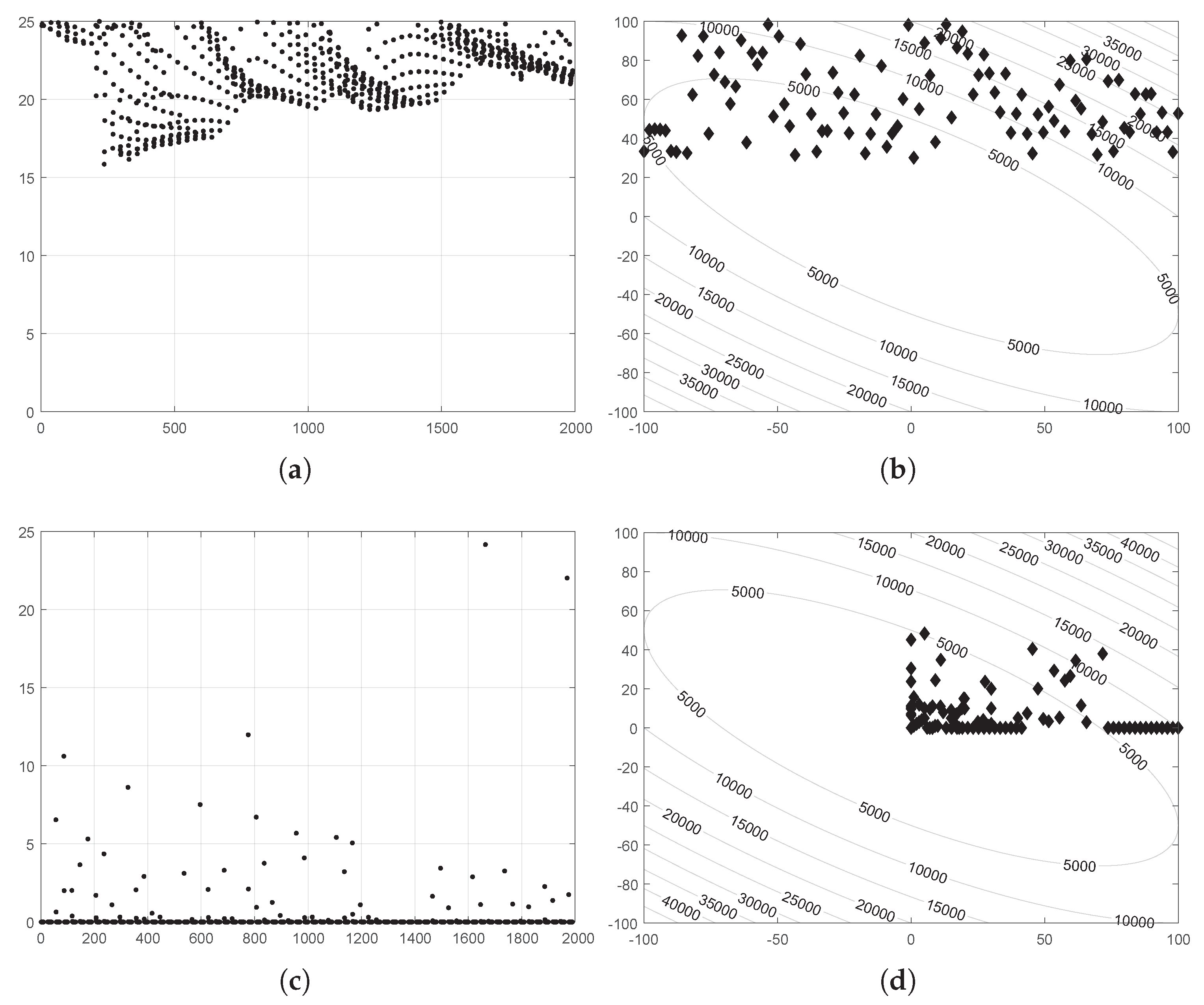
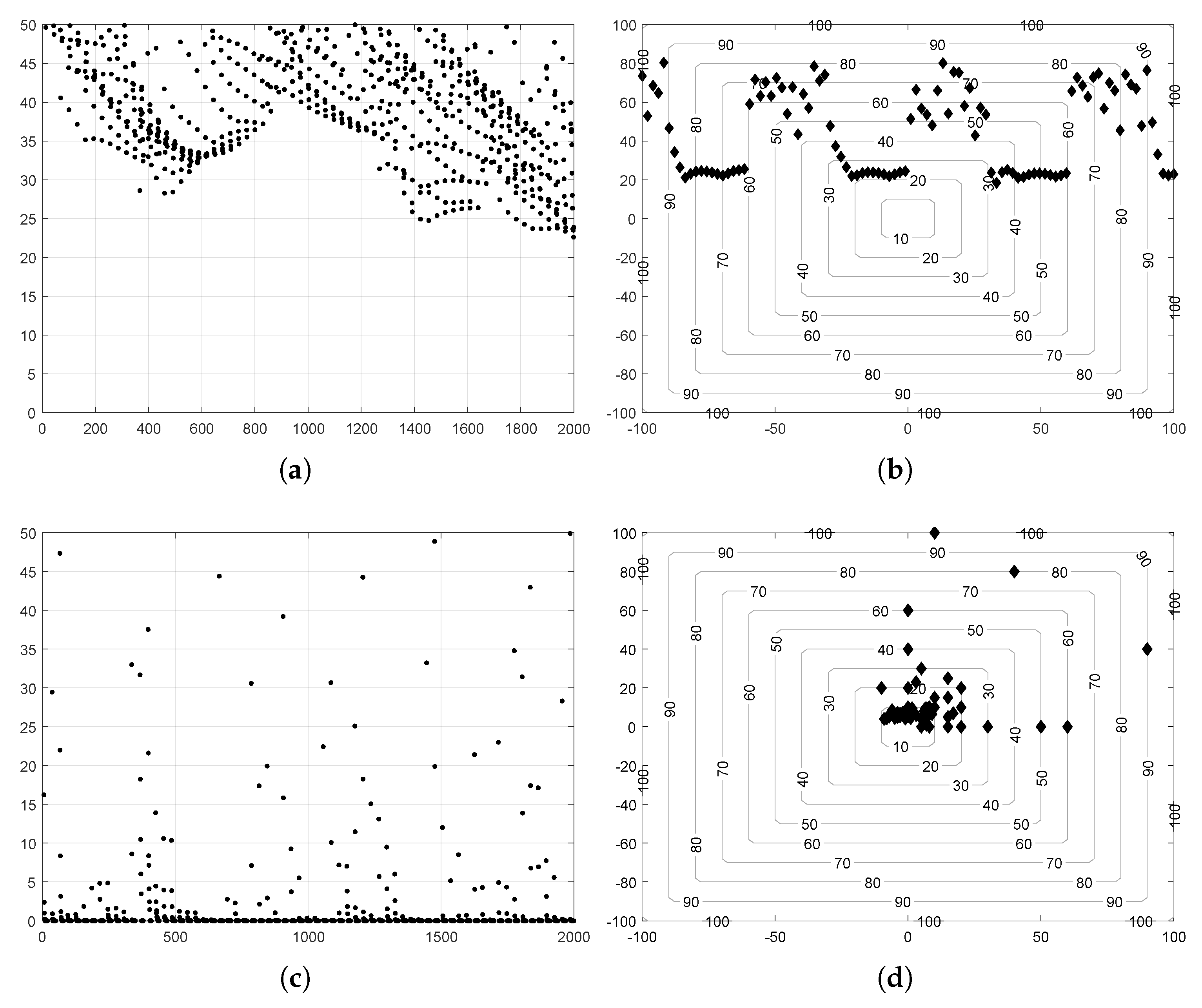
5.2. Comparison Based on Convergence

The convergence rates of the four algorithms are listed in

Table 2. MeanFES and SR by comparative algorithms for the functions $f_1-f_{16}$.

		SSA	STSSA	IWSSA	ISSA
$f_1$	MeanFES	24,699.3	23,743.1	961.8	427.1
	SR (%)	100	100	100	100
$f_2$	MeanFES	29,272.6	27,581.9	3262.9	538.5
	SR (%)	20	100	100	100
$f_3$	MeanFES	24,189.5	23,052.8	975.5	314.3
	SR (%)	100	100	100	100
$f_4$	MeanFES	28,211.3	27,320.7	2709.9	595.5
	SR (%)	100	100	100	100
$f_5$	MeanFES	NaN	NaN	NaN	NaN
	SR (%)	0	0	0	0
$f_6$	MeanFES	23,569.4	NaN	NaN	NaN
	SR (%)	100	0	0	0
$f_7$	MeanFES	NaN	22,196.0	10,977.3	16,115.1
	SR (%)	0	70	90	90
$f_8$	MeanFES	6670.3	8318.1	7208.3	7298.2
	SR (%)	100	70	40	46.7
$f_9$	MeanFES	NaN	22,598.3	765.4	342.9
	SR (%)	0	100	100	100
$f_{10}$	MeanFES	27,726.4	27,119.7	2840.9	489.7
	SR (%)	50	100	100	100
$f_{11}$	MeanFES	NaN	23,761.7	1082.5	339.9
	SR (%)	0	100	100	100
$f_{12}$	MeanFES	20,934.8	NaN	NaN	NaN
	SR (%)	63.3	0	0	0
$f_{13}$	MeanFES	21,824.07	NaN	NaN	NaN
	SR (%)	90	0	0	0
$f_{14}$	MeanFES	6371.1	2980.2	9078	6266.7
	SR (%)	97	16.67	20	24
$f_{15}$	MeanFES	10,698.4	9842.8	9280.5	11,614.1
	SR (%)	66.67	66.67	96.67	90
$f_{16}$	MeanFES	10,090.9	11,945.7	13,526	13,367.5
	SR (%)	100	100	20	33.3
Best for	MeanFES	5/16	1/16	2/16	7/16
	SR (%)	9/16	8/16	9/16	8/16

When an algorithm cannot reach an acceptable solution over the fixed number of runs, the value is marked as ‘NaN’.

. These rates are estimated using the mean number of function evaluations (MeanFES) and the success rate (SR). For most benchmark functions, ISSA presents the highest SR and the lowest MeanFES required to reach an acceptable solution. Except for ($f_6,f_8,f_{12},f_{13},$ and $f_{16}$) functions, despite the difficulty of these multimodal functions converging, ISSA nearly keeps the same values as the original SSA. For $f_7$ and $f_{15}$, the IWSSA has the best convergence speed. To manifest the convergence performance more intuitively, Figure 5 shows the convergence curves of the tested algorithms for the benchmark functions used. The ISSA presents the fastest convergence speed and the highest convergence precision compared to other algorithms for the most test functions. The ISSA can search for optimal approximation and achieve faster stability for the above benchmark functions.

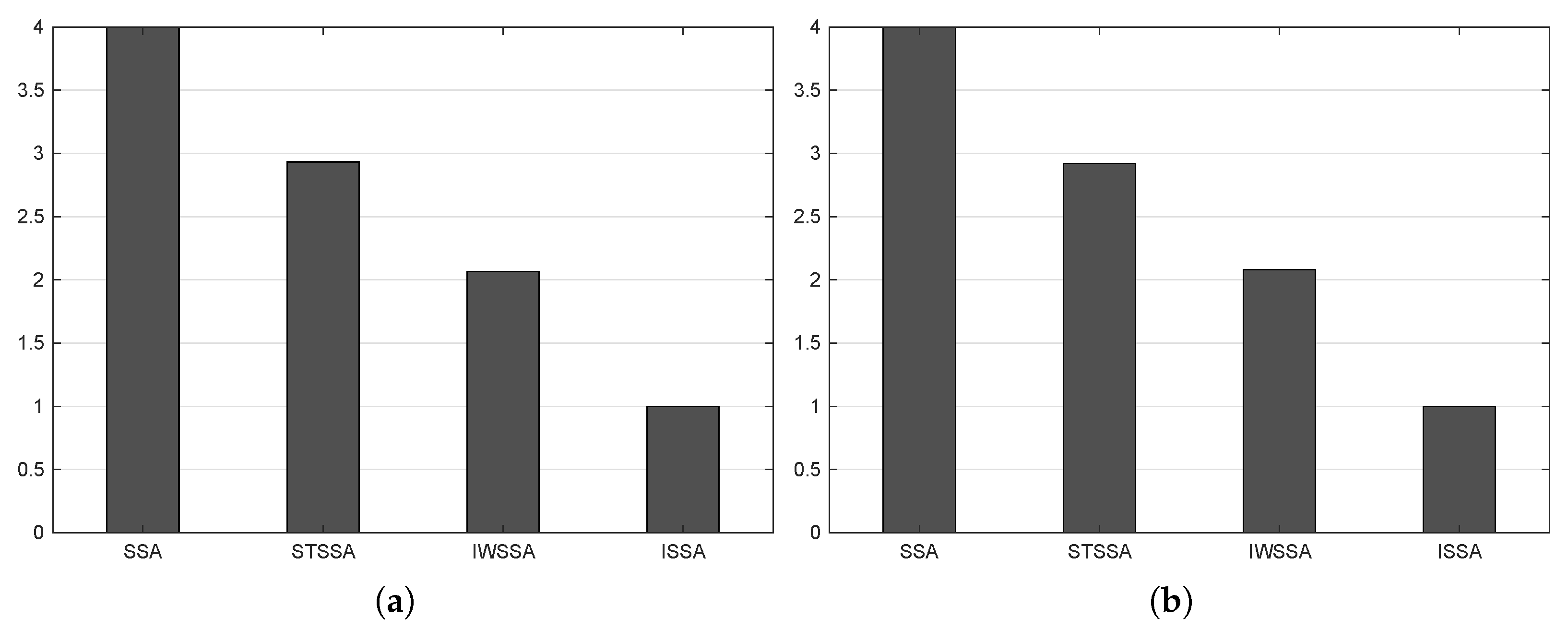
5.3. Statistical Analysis

Statistical analysis is conducted to analyze the different outcomes obtained from multiple optimization algorithms quantitatively. Since the results are not based on assumptions, we have used the non-parametric tests; Friedman and Quade tests [18,19]. Figure 6 shows the average rankings of the tested algorithms based on the standard errors of means (SEM). As it is shown in this figure, ISSA is the best ranked. In summary, the computer simulations indicate that the ISSA has an excellent ability to balance between exploration and exploitation phases and improve the whole performance of the SSA in solving the benchmark functions.

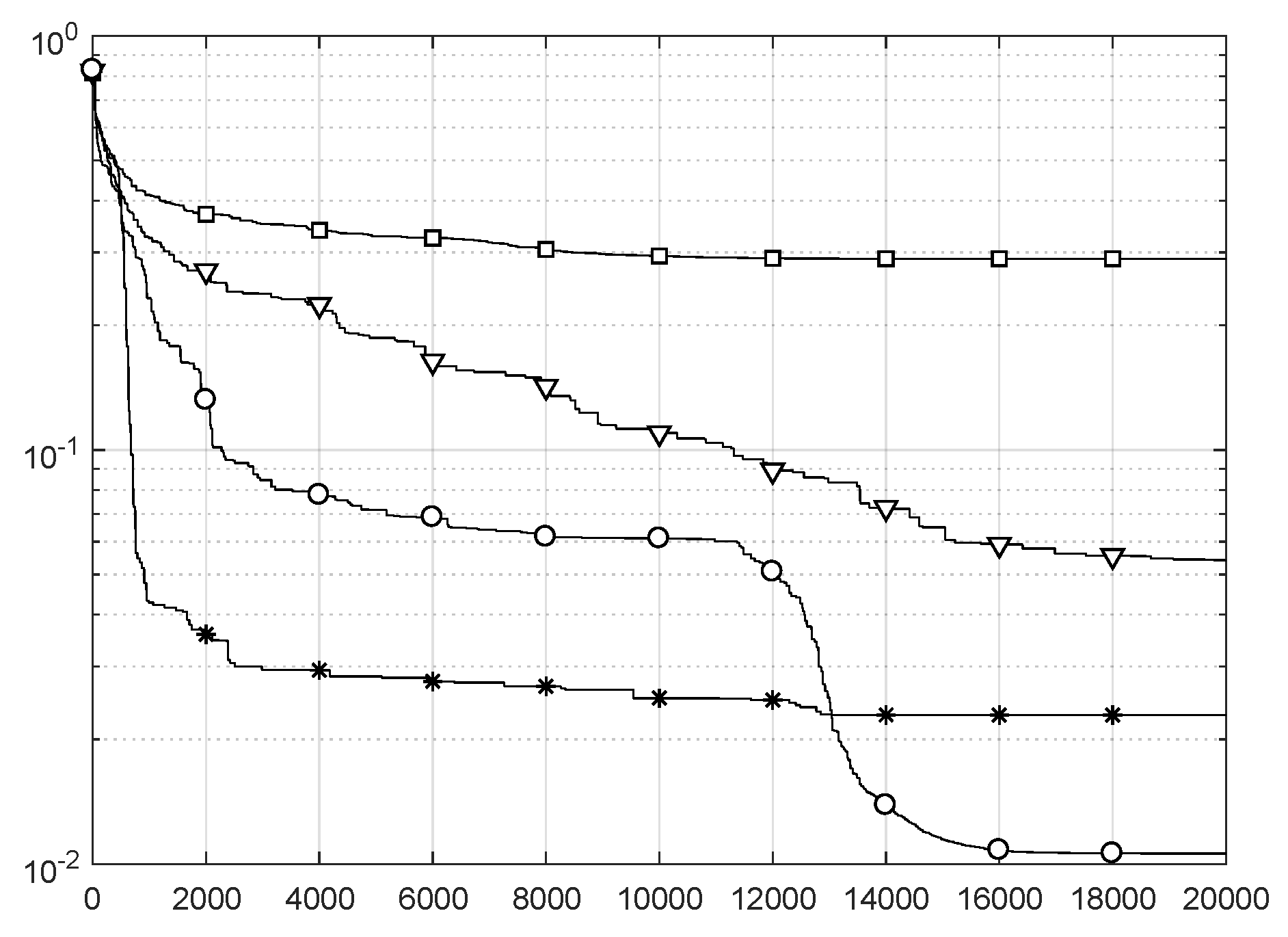
6. ISSA for Feature Weighting in DMI

To measure the performance of the proposed ISSA in providing the best feature weights for DMI, we consider the modulation pool $\varphi =\{$B-PSK, Q-PSK, 8-PSK, 4-ASK, 8-ASK, 16-QAM}, a MIMO configuration system $m\times n=2\times 6$, and a signal-to-noise ratio of 5 dB.

Table 3. Mean, SEM, and SD comparison.

	SSA	STSSA	IWSSA	ISSA
Mean	2.289 × 10${}^{-1}$	2.290 × 10${}^{-1}$	2.29 × 10${}^{-2}$	1.06 × 10${}^{-\mathbf{2}}$
SD	3.24 × 10${}^{-2}$	2.57 × 10${}^{-2}$	5.5 × 10${}^{-3}$	1.5 × 10${}^{-\mathbf{3}}$
SEM	5.9 × 10${}^{-3}$	4.7 × 10${}^{-3}$	9.954 × 10${}^{-4}$	2.801 × 10${}^{-\mathbf{4}}$

illustrates the solution accuracy for all algorithms; one can see that ISSA achieves the best mean. The convergence rate is depicted in

Table 4. MeanFES and SR comparison.

	SSA	STSSA	IWSSA	ISSA
MeanFES	NaN	10,134	810.3	2773.7
SR (%)	0	86.67	100	100

. In fact, both of ISSA and IWSSA perform better in terms of meanFES and SR. However, the plots of Figure 7 exhibit that, for a higher number of iterations, the accuracy of ISSA is much better than IWSSA, while the latter converges earlier but saturates at a greater value.

For further comparison, the classification performance of all optimization algorithms is compared to two additional cases: (i) without feature weighting (w/o FW) case and (ii) when the z-score normalization method is used as one of the most common preprocessing techniques. From

Table 5. Misclassification rate.

w/o FW	z-Score	SSA	STSSA	IWSSA	ISSA
0.1888	0.0384	0.2418	0.0213	0.0137	0.0089

, we note that the ISSA-based feature weighting approach remains the best. Confusion matrices shown in Figure 8 gives in-depth results and ensures that the proposed approach for features weighting is still the most efficient method, among the compared ones, in the considered context.

7. Conclusions

In this paper, we proposed an improved version of the SSA, dubbed ISSA, to optimize feature weighting in the context of modulation detection using an MD classifier. The ISSA relies mainly on the good balance between local and global searches through the OBL technique. Simulation results on benchmarking functions showed that the proposed algorithm widely outperforms other algorithms used for comparison in terms of solution accuracy and convergence. Thus, the validation of the ISSA through the set of benchmark functions allows its use in a wide range of optimization problems. Once used for feature weighting in DMI, as a case study, the ISSA showed better results than other approaches used for comparison, once again, in terms of solution accuracy and convergence. In fact, on average, and for moderate SNR conditions (5 dB), feature weighting using ISSA allows the following gains in correct classification rate: about 20% to the approach without feature weighting, 3% to the most used feature normalization technique, 30% to the original version of the algorithm (the SSA), and nearly 1% to the other optimization algorithms. Since it has shown a good achievement in the DMI case study, the ISSA is worthy of being applied in several wireless communications-related problems like other signal parameters detection. Moreover, this makes the ISSA a promising candidate for further preprocessing techniques in ML, such as features selection, especially since features weighting is a generalization of features selection.

References

1. Ghodratnama, S.; Moghaddam, H.A. Content-based image retrieval using feature weighting and C-means clustering in a multi-label classification framework. Pattern Anal. Appl. 2021, 24, 1–10. [Google Scholar] [CrossRef]
2. Nguyen, K.; Todorovic, S. Feature weighting and boosting for few-shot segmentation. In Proceedings of the IEEE International Conference on Computer Vision, Seoul, Korea, 27 October–2 November 2019; pp. 622–631. [Google Scholar] [CrossRef] [Green Version]
3. Tubishat, M.; Idris, N.; Shuib, L.; Abushariah, M.A.; Mirjalili, S. Improved Salp Swarm Algorithm based on opposition based learning and novel local search algorithm for feature selection. Expert Syst. Appl. 2020, 145, 113122. [Google Scholar] [CrossRef]
4. Abualigah, L.; Shehab, M.; Alshinwan, M.; Alabool, H. Salp swarm algorithm: A comprehensive survey. Neural Comput. Appl. 2020, 32, 11195–11215. [Google Scholar] [CrossRef]
5. Hodashinsky, I.; Sarin, K.; Shelupanov, A.; Slezkin, A. Feature Selection Based on Swallow Swarm Optimization for Fuzzy Classification. Symmetry 2019, 11, 1423. [Google Scholar] [CrossRef] [Green Version]
6. Parpinelli, R.S.; Lopes, H.S. New inspirations in swarm intelligence: A survey. Int. J. Bio-Inspired Comput. 2011, 3, 1–16. [Google Scholar] [CrossRef]
7. Fonseca, C.M.; Fleming, P.J. An overview of evolutionary algorithms in multiobjective optimization. Evol. Comput. 1995, 3, 1–16. [Google Scholar] [CrossRef]
8. Biswas, A.; Mishra, K.; Tiwari, S.; Misra, A. Physics-inspired optimization algorithms: A survey. J. Optim. 2013, 2013, 438152. [Google Scholar] [CrossRef]
9. Mirjalili, S.; Gandomi, A.H.; Mirjalili, S.Z.; Saremi, S.; Faris, H.; Mirjalili, S.M. Salp Swarm Algorithm: A bio-inspired optimizer for engineering design problems. Adv. Eng. Softw. 2017, 114, 163–191. [Google Scholar] [CrossRef]
10. Panda, N.; Majhi, S.K. Improved Salp swarm algorithm with space transformation search for training neural network. Arab. J. Sci. Eng. 2019, 45, 2743–2761. [Google Scholar] [CrossRef]
11. Hegazy, A.E.; Makhlouf, M.; El-Tawel, G.S. Improved salp swarm algorithm for feature selection. J. King Saud Univ. Comput. Inf. Sci. 2020, 32, 335–344. [Google Scholar] [CrossRef]
12. Kharbech, S.; Simon, E.P.; Belazi, A.; Xiang, W. Denoising Higher-Order Moments for Blind Digital Modulation Identification in Multiple-Antenna Systems. IEEE Wirel. Commun. Lett. 2020, 9, 765–769. [Google Scholar] [CrossRef]
13. Hassan, K.; Dayoub, I.; Hamouda, W.; Nzéza, C.N.; Berbineau, M. Blind digital modulation identification for spatially-correlated MIMO systems. IEEE Trans. Wirel. Commun. 2011, 11, 683–693. [Google Scholar] [CrossRef]
14. Kharbech, S.; Dayoub, I.; Simon, E.; Zwingelstein-Colin, M. Blind digital modulation detector for MIMO systems over high-speed railway channels. In Proceedings of the International Workshop on Communication Technologies for Vehicles, Lille, France, 14–15 May 2013; pp. 232–241. [Google Scholar] [CrossRef]
15. Mahdavi, S.; Rahnamayan, S.; Deb, K. Opposition based learning: A literature review. Swarm Evol. Comput. 2018, 39, 1–23. [Google Scholar] [CrossRef]
16. Ewees, A.A.; Abd Elaziz, M.; Houssein, E.H. Improved grasshopper optimization algorithm using opposition-based learning. Expert Syst. Appl. 2018, 112, 156–172. [Google Scholar] [CrossRef]
17. Mirjalili, S.; Lewis, A. The whale optimization algorithm. Adv. Eng. Softw. 2016, 95, 51–67. [Google Scholar] [CrossRef]
18. Liu, Z.; Blasch, E.; John, V. Statistical comparison of image fusion algorithms: Recommendations. Inf. Fusion 2017, 36, 251–260. [Google Scholar] [CrossRef]
19. García, S.; Fernández, A.; Luengo, J.; Herrera, F. Advanced nonparametric tests for multiple comparisons in the design of experiments in computational intelligence and data mining: Experimental analysis of power. Inf. Sci. 2010, 180, 2044–2064. [Google Scholar] [CrossRef]
Figure 1. Block diagram of the SSA.
Electronics 10 02002 g001
Figure 2. Average best solution (i.e., the achieved minimum, described by the y-axis) in terms of the number of objective function evaluations (x-axis) for the benchmark function f 3 using (a) SSA and (c) ISSA; corresponding convergence visualizations (b,d) in accordance with (a,c). (b,d) are the contour plots of the function f 3 , the x and y-axis represent the dimensions of the function, and the markers represent the evaluated points by running the optimization algorithms.
Electronics 10 02002 g002
Figure 3. Average best solution (i.e., the achieved minimum, described by the y-axis) in terms of the number of objective function evaluations (x-axis) for the benchmark function f 4 using (a) SSA and (c) ISSA; corresponding convergence visualizations (b,d) in accordance with (a,c). (b,d) are the contour plots of the function f 4 , the x and y-axis represent the dimensions of the function, and the markers represent the evaluated points by running the optimization algorithms.
Electronics 10 02002 g003
Figure 4. Block diagram of the ISSA.
Electronics 10 02002 g004
Figure 5. Average best solution (i.e., the achieved minimum, described by the y-axis) in terms of FES (the number of objective function evaluations, described by the x-axis) for the benchmark functions f 1 f 2 , f 3 f 4 , f 5 f 6 , f 7 f 8 , f 9 f 10 , f 11 f 12 , f 13 f 14 , f 15 f 16 in row-major order. Optimization algorithms are SSA [□], STSSA [▽], IWSSA [✸], and ISSA [○].
Electronics 10 02002 g005aElectronics 10 02002 g005b
Figure 6. Average ranking of comparative algorithms by Friedman test (a) and Quade test (b).
Electronics 10 02002 g006
Figure 7. Average best solution (i.e., the achieved minimum, described by the y-axis) in terms of FES (the number of objective function evaluations, described by the x-axis). SSA [□], STSSA [▽], IWSSA [✸], and ISSA [○].
Electronics 10 02002 g007
Figure 8. Confusion matrices given by (a) SSA, (b) STSSA, (c) IWSSA, (d) ISSA, (e) w/o FW, and (f) z-score.
Electronics 10 02002 g008aElectronics 10 02002 g008b