Article

A Hybrid Prognostics Deep Learning Model for Remaining Useful Life Prediction

1
School of Mechanical Engineering, Shanghai Jiao Tong University, Shanghai 200240, China
2
Faculty of Economics and Management, East China Normal University, Shanghai 200240, China
*
Author to whom correspondence should be addressed.
Electronics 2021, 10(1), 39; https://doi.org/10.3390/electronics10010039
Submission received: 2 November 2020 / Revised: 6 December 2020 / Accepted: 10 December 2020 / Published: 29 December 2020

Abstract

:
Remaining Useful Life (RUL) prediction is significant in indicating the health status of the sophisticated equipment, and it requires historical data because of its complexity. The number and complexity of such environmental parameters as vibration and temperature can cause non-linear states of data, making prediction tremendously difficult. Conventional machine learning models such as support vector machine (SVM), random forest, and back propagation neural network (BPNN), however, have limited capacity to predict accurately. In this paper, a two-phase deep-learning-model attention-convolutional forget-gate recurrent network (AM-ConvFGRNET) for RUL prediction is proposed. The first phase, forget-gate convolutional recurrent network (ConvFGRNET) is proposed based on a one-dimensional analog long short-term memory (LSTM), which removes all the gates except the forget gate and uses chrono-initialized biases. The second phase is the attention mechanism, which ensures the model to extract more specific features for generating an output, compensating the drawbacks of the FGRNET that it is a black box model and improving the interpretability. The performance and effectiveness of AM-ConvFGRNET for RUL prediction is validated by comparing it with other machine learning methods and deep learning methods on the Commercial Modular Aero-Propulsion System Simulation (C-MAPSS) dataset and a dataset of ball screw experiment.

1. Introduction

In such heavy industries as the aviation industry, the increasingly capable and advanced technologies are demanding, necessitating the reliability, intelligence, and efficiency. Those requirements, however, increase the complexity and the numbers of failure modes of the equipment.
In order to avoid the progression from an early minor failure to a serious or even catastrophic failure, reasonable preventive maintenance measures need to be taken. Traditionally, reliability indicators such as Mean Time Between Failure (MTBF) or Mean Time Before Failure (MTTF) have been assessed through reliability analysis and tests. Despite maintaining the availability of the system to some extent, conducting regular maintenance or tests has also revealed significant drawbacks: shortened intervals can cause unnecessary system downtime, regular maintenance often leads to premature replacement of components that are still functional, and excessive maintenance introduces new risks [1].
The advancements of sensor technology, communication systems, and machine learning contribute to the revolution of maintenance strategies for industrial systems, from preventive maintenance based on reliability assessment to condition-based maintenance (CBM) in numerous domains ranging from manufacturing to aerospace [2]. Considered as the key factor, CBM connects real time diagnosis of approaching failure and prognosis of future performance of the equipment, facilitating to schedule required repair and maintenance prior to the breakdown.
Referring specifically to the phase involved with predicting future behavior, prognostics and health management (PHM) is one of the enablers of the CBM. As a multi-disciplinary high-end technology that includes mechanical, electrical, computer, artificial intelligence, communication, and network, PHM uses sensors to map the equipment’s working condition, surrounding environment, and online or historical operating status, making it possible to monitor the operating status of equipment, model performance degradation, predict remaining life and assess reliability, etc., through feature extraction, signal analysis, and data fusion modeling.
In Figure 1, an implementation phase of CBM/PHM can be identified. The phase includes obtaining machinery data from sensors, signal preprocessing, extracting the features that are the most useful for determining the current status or fault condition of the machinery, fault detection and classification, prediction of fault evolution, and scheduling of required maintenance.
The goals of PHM include maximizing the operational availability, reduction of maintenance costs, and improvement of system reliability and safety by monitoring the facility conditions, and so does prognostics. The focus of prognostics is mainly on predicting the residual lifetime during which a device can perform its intended function, for example, the Remaining Useful Life (RUL) prediction. RUL is not only an estimation of the amount of time that an equipment, component, or system can continue to operate before reaching the replacement threshold, but also the indication of the health status of equipment.
If an equipment has reached the end of its service life, the number and complexity of environmental parameters (e.g., temperature, pressure, vibration levels, etc.), in which the equipment operates can significantly affect the accuracy of the prediction. An accurate RUL prediction is significant to the PHM, since it provides benefits, which, in turn, improve the decision-making for operations and CBM.
Aiming to predict the RUL of equipment, numerous methods are proposed, which contain two major branches: physical models and data-driven methods. The overview is shown in Figure 2.

1.1. RUL Prediction Based on Physical Models

The degradation trend can be determined by such physical theories as fatigue damage theory and thermodynamics theory. Hoeppner et al. propose a fatigue-crack growth law, combining the knowledge of fracture mechanics to illustrate the application of fatigue-crack growth model [3]. Contemporary, with the complexity and integration of advanced equipment, the RUL of equipment can be estimated by numerical integration using different fatigue crack growth rate. To overcome such a difficulty, Mohanty et al. propose an exponential model that can be used without integration of fatigue crack growth rate curve [4]. To analyze the fatigue of pipelines, Divino et al. present a method based on nominal stresses, using a one-dimensional Finite Element mode with the application of stress concentration factors. The results make sense for not only finding the appropriate model, but also predicting the RUL through temperature theory [5]. By evaluating the axial natural frequency from the motor current signal and axial vibrational signal, Nguyen et al. propose a discrete dynamic model to characterize the degradation level [6]. The physical-model-based approach is suitable for a specific subject where the failure mechanism is well defined. Once an accurate physical model has been developed based on the system characteristics, the accuracy of the RUL prediction method is high, and the method is highly interpretable because it corresponds to the physical quantities through a mathematical model. However, as the structure of the equipment system becomes more and more complex, those physical models, mainly focusing on exploiting the fault mechanism of the equipment, may not be the most feasible for practical prognostic of complex equipment, for example, the turbofans or the ball screws, since the uncertainty in the machining process and the measurement noise are not incorporated in the physical models, and it is difficult to perform extensive experiments to identify some model parameters.

1.2. RUL Prediction Based on Data-Driven Method

Data-driven methods concentrate on the degradation of equipment from monitoring data instead of building physical models. To monitor the operating condition in all directions, the system is often equipped with a number of measuring sensors, making the data for data-driven methods high dimensional. Yan et al. provided a survey on feature extraction for bearing PHM applications [7,8]. High frequency resonance technique (HFRT) is a widely used frequency domain technique for bearing fault diagnosis [9]. The Hilbert–Huang Transform (HHT) and Multiscale entropy (MSE) are used to extract features and evaluate the degradation levels of the ball screw [10]. Feature learning is a method which transforms the extracted features into a representation that can be effectively exploited in data-driven methods. Hinton and Salakhutdinov [11] proposes auto-encoders to learn features of handwriting, which is a commonly used unsupervised method in transfer writing.
According to the characteristics of RUL as a non-linear function, the current data-driven methods for RUL prediction are mainly divided into three branches: statistical model methods, machine learning methods represented by back propagation neural network (BPNN), and deep learning methods represented by long short-term memory (LSTM). The statistical model-based model assumes that the RUL prediction process is a white-box model, by inputting the device history data into the established statistical degradation model, and continuously adjusting the degradation model parameters to update the model accuracy. Based on existing information to establish probability density distributions for battery states, Saha et al. apply Bayesian estimation to battery cycle life prediction to quantify the uncertainty in RUL predictions [12]. Bressel presents an HMM-based method, from which a state transfer matrix is obtained through matching tracing down [13].
The actual engineering applications in the degradation model, however, often cannot be determined in advance, and different equipment has different working conditions, the inappropriate selection of degradation model will greatly affect the accuracy of the prediction results, thus causing huge economic losses [14]. Machine learning methods are mostly grey-box models that do not require a prior degradation model, and the input data are not limited to the historical usage data of the device [15,16,17]. Guo et al. propose a rolling bearing RUL prediction method based on improved deep forest, the model first iteratively calculates the equipment usage data by fast Fourier transform, and then replaces the traditional random forest multi-grain scan structure with a convolutional neural network, thus predicting the remaining life of rolling bearings [18]. Celestino et al. propose a hybrid autoregressive integrated moving average–support vector machine (ARIMA–SVM) model that first extracts features from the input data via the ARIMA part, and then feeds the extracted features into the SVM model to predict the remaining lifetime [19]. Based on singular value decomposition (SVD), Zhang et al. perform feature extraction of rolling bearing historical data to evaluate bearing degradability [20]. Yu et al. improve the accuracy of the prediction of bearing remaining life by improving the recurrent neural network (RNN) model by zero-centering rule [21].
Faced with massive amounts of industrial data, the computing power and accuracy of some machine learning models cannot meet industrial standards [22]. Hence, deep learning is adopted universally to extract the features in non-linear systems [23]. Deep learning models, such as LSTM, are widely used for their long-term memory capabilities. Elsheikh et al. combined deep learning with long and short memory to derive a deep long short-term memory (DLSTM) model, which firstly explored the correlation between each input signal through deep learning model, and then introduced random loss strategy to accurately and stably predict the remaining service life of aero-engine rotor blades [24]. Based on the ordered neurons long short-term memory (ON-LSTM) model, Yan et al. first extracted the health index by calculating the frequency domain features of the original signal; then constructed the ON-LSTM network model to generate the RUL prediction value, which uses the sequential information between neurons and therefore has enhanced prediction capability [25]. Though effective, RNN derived methods have the problem of gradient explosion, significantly affect the accuracy of the methods. Cho et al. proposed the encoder–decoder structure, which can learn to encode a variable-length sequence into a fixed-length vector representation and decode a given fixed-length vector representation back into a variable-length sequence [26]. To remedy the gap between the emerging neural network-based methods and the well-established traditional fault diagnosis knowledge because data-driven method generally remains a “black box” to researchers, Li et al. introduce attention mechanism to assist the deep network to locate the informative data segments, extract the discriminative features of inputs, and visualize the learned diagnosis knowledge [27]. Zhou et al. proposed the attention-mechanism-based convolutional neural network (CNN), with positional encoding, to tackle the problem that RNNs take much time for information to flow through the network for prediction [28]. The attention mechanism enables the network to focus on specific parts of sequences and positional encoding injects position information while utilizing the parallelization merits of CNN on GPUs. Empirical experiments show that the proposed approach is both time effective and accurate in battery RUL prediction. Louw et al. combine dropout with Gate Recurrent Unit (GRU) and LSTM to predict RUL, obtaining an approximate uncertainty representation of the RUL prediction and validating algorithmically the turbofan engine dataset [29]. Liao et al. propose a method based on Bootstrap and LSTM, which uses LSTM to train the model and obtains the confidence intervals for RUL predictions [30].
Admittedly, LSTM has the capability to deal the signal and predict RUL. With the large data and equipment operating under various conditions, the calculating speed and accuracy was undermined because the changeable conditions could influence the prediction and only with faster and more quick-responsible method can we get more accurate RUL prediction results. To achieve more competitive prediction results, Kyunghyun et al. propose a Gate Recurrent Unit (GRU) [31]. They couple the reset (input) gate to the update (forget) gate and show that this minimal gated unit (MGU) achieves a performance similar to the standard GRU with only two-thirds of the parameters, overcoming the risk of overfitting. GRU is a binary convolutional neural network whose weights are recursively applied to the input sequence until it outputs a single fixed-length vector. Compared to LSTM, GRU only reserves two gates, namely the forget fate and output gate, and has faster calculating speed than that of LSTM.
To further develop the value of gates of recursive convolutional neural network, a two-phase deep-learning-model attention-convolutional forget-gate recurrent network (AM-ConvFGRNET) for RUL prediction is proposed. The first phase, forget-gate recurrent network (FGRNET) is based on a one-dimensional analog LSTM, which removes all the gates except the forget gate and uses chrono-initialized biases [
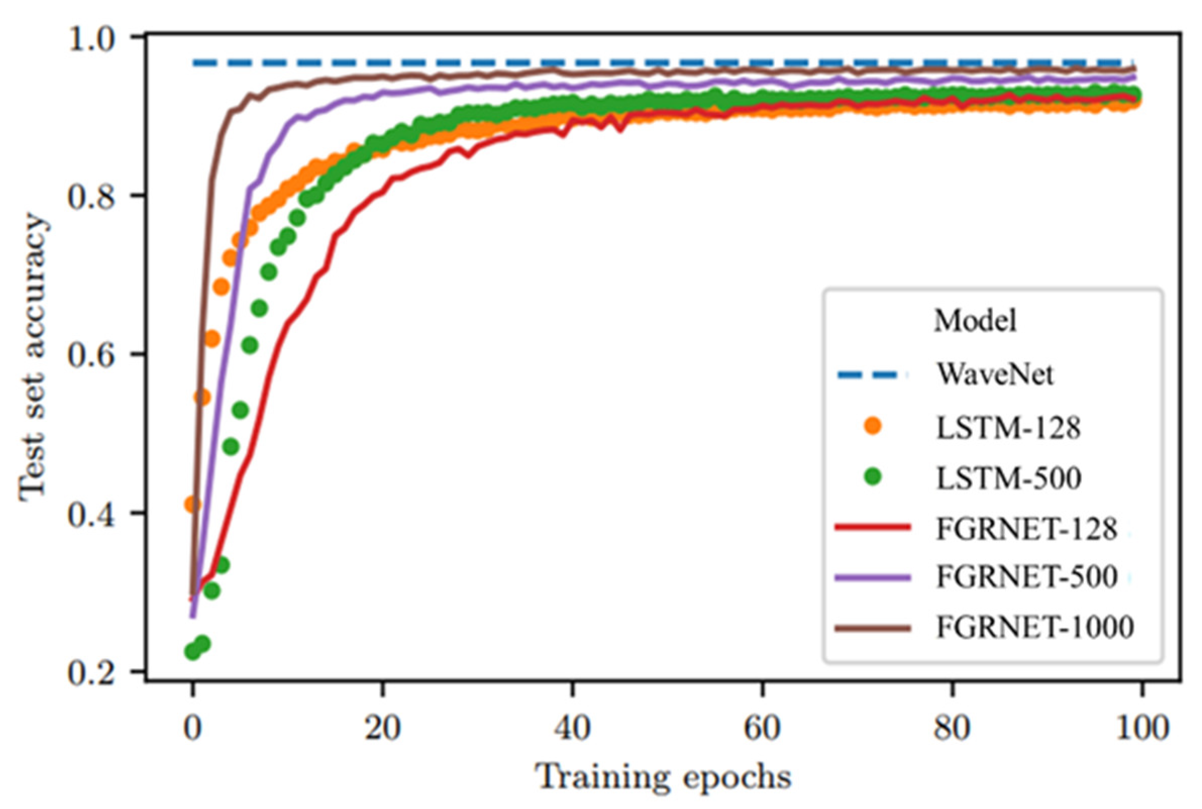
32]. The combination of fewer nonlinearities and chrono-initialization enables skip connections over entries in the input sequence. The skip connections created by the long-range cells allow information to flow unimpeded from the elements at the start of the sequence to memory cells at the end of the sequence. For the standard LSTM, however, these skip connections are less apparent and an unimpeded propagation of information is unlikely due to the multiple possible transformations at each time step. The fully connected layer is then added into the FGRNET model to assimilate temporal relationships in a group of time series. The FGRNET model is transformed into ConvFGRNET. The second phase is the Attention Mechanism: The lower part is the encoder structure which employs bi-directional recurrent neural network (RNN), the upper part is the decoder structure, and the middle part is the attention mechanism. The proposed model is capable of extracting more specific features for generating an output, compensating the drawbacks of the ConvFGRNET that it is a black box model and improving the interpretability. Hence, a two-phase model is proposed to predict the RUL of equipment. To comprehensively evaluated the performance of the proposed method, the ability of classification of FGRNET is first tested on MNIST (a database of handwritten digits performed) dataset [33], whose result is then compared with RNN, LSTM and WaveNet [34]. Then, the strengthen of RUL prediction is demonstrated through experiments dependent on a widely used dataset, and comparisons with other methods. To further evaluate, an experiment based on ball screw is conducted and proposed method is tested.
The main innovations of the proposed model are summarized as follows:
  • The proposed AM-ConvFGRNET simplifies the original LSTM model, in which the input and output gates are removed and only a forget gate is retained to correlate data accumulation and deletion. The simplified gate structure ensures the model could construct complex correlations between device history data and its remaining life, and to achieve faster gradient descent and increased computing power.
  • The attention mechanism is embedded into the ConvFGRNET model, which can increase the receptive field for feature extraction, increasing the prediction accuracy.
The article is developed as follows. The AM-ConvFGRNET is discussed in Section 2. The data features and the data processing are discussed in Section 3. The experiments and validation of the model is discussed in Section 4. The conclusion is addressed in Section 5.

2. The Proposed Model

The model proposed contains four major parts: data input, FGRNET feature learning, health status assessment, and RUL prediction. The accuracy of the prediction is characterized by calculating the RMSE. Detailed calculation is shown as follows, and the process is in Figure 3.

2.1. Initialization of the Input Data

Given the input data, Ω = { ( x i t j , y i ) } i = 1 N , where Ω represents the dataset; N represents the number of training samples; x i t j T × D represents a time window with D eigenvalues and a timeseries range of T ;   y i represents the Remaining Useful Life of the turbo fan since x i t j .

2.2. Initialization of Training Model Parameters

Maximum likelihood estimation was used to select the parameters θ = { w 1 ,   w 2 ,   ,   w n } . Assuming that the N training samples are independently co-distributed. By inserting a Gaussian transform with several large likelihood functions, the distribution of model parameters obeys the function shown as follows:
l ( θ ) = i = 1 N log [ ( 1 2 π σ 2 ) 1 2 exp ( 1 2 π σ 2 ( y i μ ( x i ) ) 2 ) ] = 1 2 σ 2 ( x ) i = 1 1 ( y i μ ( x i ) ) 2 N 2 log ( 2 π σ 2 ( x ) )
The model proposed itself is a learning process through which the dataset Ω = { ( x i t j , y i ) } i = 1 N is input and then is mapped as x i T × D y i . Moreover, Ω can be used first for learning the a priori model P ( y   | x ,   θ ) and then for training the AM-FGRNET model:
x i y i * + ε i = argmax   log   P ( y i x i , μ ( x i ) , σ 2 ( x i ) )

2.3. Model Training

First, running the AM-ConvFGRNET model, then mapping the historical run data to the RUL predicted value, y i , and finally building the loss function as follows:
E n = i = 1 B ( y i y i * ) 2
where B is the size of each batch split by the training sample size, y i is the model predicted RUL value, and y i * is the real RUL. The gradient descent method is then used to optimally adjust the model parameters selected based on the maximum likelihood estimation.

2.4. RUL Prediction

The dataset to be processed according to Equations (1)–(3) will first be constructed with a data matrix, and then the constructed matrix will be entered into the AM-ConvFGRNET network to calculate the RUL of the equipment. All the symbols used in the equations can be found in Table 1.

2.5. FGRNET Structure

A recurrent neural network (RNN) creates a lossy sequence summary h T , The main reason why h T is lossy is that RNN maps an arbitrarily long sequence x 1   :   T to a vector of fixed lengths. Greff and Jozefowicz proposed the addition of a forget gate to the LSTM in 2015 to address such issues [35]:
i t = σ ( U i h t 1 + W i x t + b i )
o t = σ ( U o h t 1 + W o x t + b o )
f t =   σ ( U f h t 1 + W f x t + b f )
c t = f t c t 1 + i t tanh ( U c h t 1 + W c x t + b c )
h t = o t tan h ( c t )
In the formulas, x t is the input vector of the time node, t , moment; U i ,   U o ,   U f , and U c are the regular weight matrix between the input and the hidden layer; W i ,   W o ,   W f , and W c are a matrix of recursive weights between the hidden layer and itself at the adjacent time step; vectors b i ,   b o ,   b f , and b c are bias parameters which allow each node to learn bias; h t represents the vector, of which hidden layer is at time node, t ; h t 1 is the value of the previous output of each memory cell in the hidden layer; represents dot-multiply; σ is the sigmoid function; and i t and o t represent the vectors of input gate and output gate at the t moment, respectively.
To better develop the advantages of the forget gate, based on classical LSTM model [36], FGRNET model is proposed. Such a model removes the input gate and output gate, and only set a forget gate. Jos and Joan then combined the input and forget mechanism modulation to achieve the pheromone accumulation and association.
On the one hand, because the t a n h activation function of h t causes the gradient to shrink during back propagation, thus exacerbating the vanishing gradient problem on the other hand, because the weight value U * may accommodate values outside the range [−1,1], we can remove the unnecessary, potentially problematic t a n h nonlinear function. The structure of FGRNET is shown as below:
f t = σ ( U f h t 1 + W f x t + b f )
c t = f t c t 1 + ( 1 f t ) tanh ( U c h t 1 + W c x t + b c )
h t = c t
In commonplace, having the accumulation of information slightly more than that of forgotten is feasible, making the analysis of time sequence more easily. According to the empirical evidence, it is feasible to subtract a predetermined value of β from the component of the input control variable:
f t = U f h t 1 + W f x t + b f
  c ˜ t = tanh ( U c h t 1 + W c x t + b c )
c t = σ ( s t ) c t 1 + ( 1 σ ( s t β ) )   c ˜ t
h t = c t
where f t represents the forget gate;   c ˜ t is the representation of new storage cells acquired by the model from forgotten information; c t is the information storage cells before forgetting; h t is the hidden layer in the model.
In the FGRNET model, β is often independent of the dataset, Westhuizen et al. proved that, when β = 1 , the performance of the model is the best [37].
The flowchart of the FGRNET model is shown in Figure 4, in which the information fluxes in the loop unit is demonstrated as well. Unlike the RNN and LSTM models, FGRNET is only able to share information in the hidden state:

2.5.1. Initialization of Forget Gate

Focusing on the forget gate bias of LSTM, Tallec and Ollivier [32] proposed a more appropriate initialization method called chrono-initialization, which begins with the improvement of the leakage unit of the RNN [38]:
h t + 1 = α tan h ( Uh t + Wx t + b ) + ( 1 α ) h t
Through the first-order Taylor expansion, h ( t   +   δ t ) h ( t ) + δ t d h ( t ) d t , and the addition of the discrete units δ t = 1 , we get the following formula:
d h ( t ) d t = α tanh ( Uh ( t ) + Wx ( t ) + b ) α h ( t )
Tallec [32] proved that in the free regime, after a certain time node t 0 , the input stops, we have x ( t ) = 0 ,   ( t > t 0 ) ; then we set b = 0 ,   U = 0 , and Formulas (12)–(14) turn into the following:
dh ( t ) d t = α h ( t )
t 0 t 1 h ( t ) dh ( t ) = α t 0 t d t
h ( t ) = h ( t 0 ) exp ( α ( t t 0 ) )
According to the Formulas (18)–(20), the hidden state h will reduce to e 1 of its original value in the time proportional to 1 / α , where 1 / α can be viewed as the characteristic forgetting time, or a constant, of the recurrent neural network. Hence, when modeling a timeseries that has dependencies in the range [ T m i n ,   T m a x ] , the forgetting time of the model used should lie in roughly the same time frame, i.e., the α [ 1 T m a x ,   1 T m i n ] d , where d is the hidden cell.
As to the LSTM, the time-varying approximation of α and ( 1 α ) are respectively learned by the input gate i and the forget gate f .
Then we apply the chrono-initialization on the forget gate of the FGRNET, whose active function is as follows:
σ ( log ( T m a x 1 ) ) = 1 1 + exp ( log ( T m a x 1 ) T m a x 1
The chrono-initialization can fulfill the skip-like connections between the memory cells, mitigating the vanishing gradient problem.

2.5.2. Gradient Descent Function of FGRNET

Combining the Equations (1)–(8), the pre-activation function can be written as follows:
S i , o , f , c = U i , o , f , c h t + W i , o , f , c x t + 1 + b i , o , f , c
The memory units of single-layer FGRNET is compared with single-layer LSTM, and then make an analysis through calculating the objective function J and the differential J c t of an arbitrary memory vector c t . The Functions (6) and (7) can be rewritten as follows:
f t + 1 = σ ( s f )
c t + 1 = f t + 1 c t + ( 1 f t + 1 ) tanh ( s c )
The gradient descent function of the objective function J is characterized as follows:
J c t = J c T k = t T 1 [ c k + 1 c k ]
where
c t + 1 c t = U f σ ( s f ) c t + σ ( s f ) + ( 1 σ ( s f ) ) ( U c tanh ( U c c t ) ) σ ( s f ) ( U f tanh ( U c c t ) )
As the time series follows, both the input and the hidden layer converge wirelessly to 0, which means that σ ( s f ) converges to 1. Hence, Equation (26) can be reduced to c t + 1 c t 1 , which means that the gradient of the memory unit c t is not affected by the length of the time series.
For example, a network whose structure is n 1 × n 2 and the numbers of the input and the hidden cells are n 1 and n 2 respectively. Classical LSTM model contains 4 elements: input gate, output gate, forget gate, and the memory vector, j = { i ,   o ,   f ,   c } , and the number of the total elements are 4 ( n 1 n 2 + n 2 2 + n 2 ) . Compared with the LSTM, FGRNET contains only two elements, the forget gate and the memory vector, j = { f ,   c } , and the number of total elements is 2 ( n 1 n 2 + n 2 2 + n 2 ) , which is reduced to a half to that of the LSTM.
To demonstrate the superb characteristics of FGRNET, an experiment based on a public dataset is conducted. Because later the prediction part will be discussed, the MNIST experiment shows the superb ability of FGRNET for classification, making a pre-validation for the feasibility of FGRNET.
These public data contain the MNIST, permuted MNIST (pMNIST) [33], and MIT-BIH (a database for the study of cardiac arrhythmias provided by the Massachusetts Institute of Technology) arrhythmia datasets [39]. Through BioSPPy package, single heartbeats are extracted from longer filtered signals on channel 1 of the MIT-BIH dataset [40]. The signals were filtered by using a bandpass FIR filter between 3 and 45 Hz. Four heartbeat classes which can present different patients are chosen: normal, right bundle branch block, paced, and premature ventricular contraction. The dataset contains 89,670 heartbeats, each of length 216 time steps. The dataset is set according to the rule (70:10:20), which is also applied on MNIST dataset.
For the MNIST dataset, a model with two hidden layers of 128 units is performed, whereas a single layer of 128 units was used for the pMNIST. The networks are trained through Adam [41] with the learning rate of 0.001 and a mini-batch whose size is 200. The output of the recurrent layers is set as 0.1 and the weight decay factor is used as   1 × 10 5 . The training epoch is set as 100 and the best validation loss was employed to determine the performance of the model. Furthermore, the gradient norm was clipped at a value of 5.
Table 2 presents the results of three datasets. In additional to FGRNET and LSTM, RNN and other RNN modifications are demonstrated as well. The means and standard deviations from 10 independent runs are reported.
It is indicated that FGRNET is better than the standard LSTM, and is among the top performing models of the analyzed dataset.
Larger layer sizes are experimented. In Figure 5, the test set accuracies during training for different layer sizes of the LSTM and the FGRNET are illustrated. Moreover, a well-performed accuracy (96.7%) achieved by WaveNet is also demonstrated [34]. The FGRNET clearly improves with a larger layer and performs almost as well as the WaveNet.
The effectiveness of FGRNET could be attributed to the combination of fewer nonlinearities and chrono initialization. This combination enables skip connections over entries in the input sequence. the skip connections created by the long-range cells allow information to flow unimpeded from the elements at the start of the sequence to memory cells at the end of the sequence. For the standard LSTM, these skip connections are less apparent and an unimpeded propagation of information is unlikely due to the multiple possible transformations at each time step.

2.6. Convolutional FGRNET

To enhance the ability of LSTM to deal with sequence data and make the feature extraction better, Graves proposes a fully connected LSTM (FC-LSTM) [45]. However, FC-LSTM layer, on the one hand, adopted by the model does not take spatial correlation into consideration; Although the FC-LSTM layer has proven powerful for handling temporal correlation, it contains too much redundancy for spatial data on the other.
Based on FC-LSTM, Shi et al. proposes the Convolutional LSTM (ConvLSTM), which appears with the purpose that a LSTM network takes into account nearby data, both spatially and temporally [46]. The mechanism of ConvLSTM is shown from Formulas (27)–(29):
(1)
When an input X t arrives, the input gate i t , the forget gates f t , the new memory cell C t are obtained.
i t = σ ( W i X t + Ui H t 1 + V i C t 1 + b i )
f t = σ ( W f X t + U f H t 1 + V f C t 1 + b f )
C t = tanh ( W c x t + U c h t 1 + b C )
where * is the convolutional operation and is the Hadamard product.
(2)
The output gate, O t , is computed as follows:
O t = σ ( W o X t + U o H t 1 + V o C t 1 + b o )
(3)
Hidden state, h t j , is calculated as follows:
H t = O t tanh ( C t )
In the same way that the ConvLSTM has been proposed, the ConvFGRNET is proposed, which is used to assimilate temporal relationships in a group of time series.
(4)
An input X t arrives, and the forget gate, f t j , is obtained as follows:
f t = σ ( W f X t + U f H t 1 + b f )
(5)
The new memory cell is created and added:
C t = f t C t + ( 1 f t ) tanh ( W c X t + U c H t 1 + b c )
(6)
The state of the hidden layer is calculated as follows:
H t = C t
The active function of fully connected layer is chosen as s i g m o i d , which is used to evaluate the health of the equipment, estimating the RUL. The calculation of fully connected layer can be defined as follows:
p = σ ( w f · H ( t ) + b p )
where the output is the decimal between 0 and 1, indicating the health status of the equipment; H ( t ) is the output of the hidden layer; w f is the weight value of the fully connected layer; and b p is the bias.
The structure of ConvFGRNET is shown in Figure 6.

2.7. AM-FGRNET

Although the ConvFGRNET can achieve better generalization than the LSTM does on synthetic memory tasks, it cannot process multi-data series simultaneously. Hence, it is difficult for ConvFGRNET to learn the relationships among time series, meaning that RUL prediction in sophisticated equipment cannot be accurately performed because it cannot deal time series and relations between variables.
In view of those considerations, attention mechanism is employed and embedded into ConvFGRNET model. The AM-ConvFGRNET model is shown as Figure 7.
In the attention mechanism, the lower part is the decoder structure, which is composed by bi-directional RNN, with forward RNN inputting signal in order, while backward RNN inputting signal verse order. Splicing the hidden states of two RNN units at the same time to form the final hidden state output h t , which contains not only the information of the previous moment of the current signal, but also contains that of the next moment. The upper part is the Encoder structure, which is a uni-directional RNN. The middle part is attention structure, which is calculated as follows:
c i = j = 1 T x a i j h j
The weight α i j of each annotation h j is computed by the following:
a i j exp ( e i j ) k = 1 T x exp ( e i k )
where e i j = a ( s i 1 ,   h j ) .

2.8. Health Status Evaluation

After combing the information and calculating, the learned feature information is smoothed into 1D feature data, and then the data are input into the fully connected network and calculated as follows:
p = σ ( w f · H t + b p )
where p is the output of the fully connected layer, and is a number between 0 and 1, indicating the health status of the equipment; σ is the active function which is chosen as s i g m o i d ; w f is the weight value in the fully connected layer; H t   i s   t h e   i n p u t ,   a n d   i s   t h e   o u t p u t   o f   h i d d e n   l a y e r ;   b p is the bias.

2.9. RUL Prediction

The remaining life of the current equipment can be predicted based on its performance parameters and historical operation data. Combined with the health status p of the equipment, the historical operating time series can be used to predict the RUL. y i represents the remaining life of the current equipment at t moment. y i is calculated as follows:
y i = inf ( y : p ( H t ) γ ) + ε
where inf ( · ) is the lower limit of the variable; f ( H t ) is the health status of the equipment at the moment H t ; γ is the failure threshold; ε represents the errors arising from network models. According to Sateesh Babu [47], Li [48], and Zhang et al. [49], ε obeys the normal distribution:
ε ~ N ( f ( H t ) ,   σ 2 ( x i ) )
where   σ 2 ( x i ) is the variance of prediction error.
The health state of the equipment is characterized by a number between 0 and 1, with 1 being the failure threshold. t is the current running time, and p ( H t ) is the current health state of the machine. Hence, RUL can be written as follows:
y i = t p ( H t ) t
Because the remaining life of the equipment is influenced by various factors, the predictions are probabilistically distributed. Moreover, the values and the distributions of the predictions can be obtained through multi-calculations, from which the accuracy of the tested model can be achieved as well.

2.10. Evaluation Indications

RMSE and Score [50] are chosen as the evaluation benchmark of the prediction results, whose definitions are shown as below.
RMSE:
i = 1 n ( d ) 2 n
This matric is used to evaluate prediction accuracy of the RUL. It is commonly used as a performance measure since it gives equal weights for both early and late predictions.
Score:
s = { i = 1 n e ( d a 1 ) 1   for   d < 0   i = 1 n e ( d a 2 ) 1   for   d 0
where s is the score (cost) of the model; n is the is the number of units in the test set; d is the difference between the predicted values and the real values, d = R U L i ¯ R U L i (estimated RUL − true RUL, with respect to the i t h data point). a 1 and a 2 are the constant coefficients and are set as 10, 13 respectively. The higher the score, the greater the deviation of the model prediction from the true value.
The characteristic of this scoring function lean towards early predictions (i.e., the estimated RUL value is smaller than the actual RUL value) more than late predictions (i.e., the estimated RUL value is larger than the actual RUL value) since late prediction may result in more severe consequences.
Using RMSE in conjunction with the scoring function would avoid to favor an algorithm which artificially lowers the score by underestimating it but resulting in higher RMSE.
Figure 8 illustrates the differences between the scoring function and the RMSE function.

3. Case Study

3.1. Commercial Modular Aero-Propulsion System Simulation (C-MAPSS) Dataset

Considering the difficulty of collecting the operating data during the full life cycle of a turbo engine, NASA uses a software called Commercial Modular Aero-Propulsion System Simulation (C-MAPSS) to simulate the working condition of turbofan and then to generate the data. C-MAPSS is able to simulate the Pratt & Whitney F100 turbofan under different operating conditions and different types of failure modes, and it can simulate the degradation of different turbofan components by varying the operating conditions of the equipment, controlling the equipment parameters, and adding different levels of noise in each simulation.
C-MAPSS then generates four sets of time series with sequential increases in complexity. In each time series, the behavior of the turbofan is shown for 21 parameters of sensors of the system and other three parameters that show turbofan’s operating conditions. The number of failure modes and operating conditions are summarized in the Table 3.
Included in FD001 are 21 sensor signals and three parameters. Those features consist of four temperature measurements, four pressure measurements, and six angular velocity measurements. Comprehensively, those 24 measurements reflect the operation conditions of subsystems in the turbofan. Hence, from the C-MAPSS dataset, RUL can be predicted. The detailed list is shown in Table 4.
Each turbofan begins with different degrees of initial use and unknown manufacturing conditions although this initial use and manufacturing conditions are considered normal, i.e., it is not considered a failure condition [51].
Hence, turbofan’s sequences shown normal or nominal behavior at the beginning of each time series and in some point begin to degrade until predefined limit in which it is considered that the turbofan can no longer be used.
In this work, the method which retains RUL greater than a certain number of cycles as constant is considered feasible. This makes sense because the parameters showing turbofan behavior would show normal operating conditions at those points, i.e., the data show a slight variation, reducing the feasibility of making different and accurate predictions for each point.
In contrast, the data since the failure reveal a lot of information and allow for the best results. It is then assumed that there is a time from the start of the run, so that with 99% probability the turbofan is working properly.

3.1.1. Parameter Analysis

Figure 9 and Figure 10 demonstrate that signals can have different characteristics based on the operation stage of the turbofan. For example, outlet temperature of high-pressure compressor generally increases with the number of operating cycles, while the actual angular velocity of core machine decreases. Hence, when considering improve the RUL prediction of the turbofan, elements should be comprehensively employed since different elements reflect the status of the engine.
In each dataset, the correlations between parameters influence the health status evaluation, so as the RUL prediction. Given the complex structure of the turbofan engine, the correlations between each element during operation vary. Figure 11 shows the Pearson correlation coefficient between each element in FD001. The white and black part indicate the strong positive and negative correlations; the red part means weak correlation.
From Figure 11, it is obvious that in FD001, inlet temperature of fan ( C 1 ) is correlated strongly with bypass pressure of pipeline ( C 6 ), oil to gas ratio of combustion chamber ( C 16 ), while outlet temperature of low-pressure compressor ( C 2 ) is with outlet temperature of low-pressure turbine ( C 4 ), ratio of fuel flow to static pressure of high-pressure-compressor outlet ( C 12 ), and cooling flow of low-pressure turbine ( C 21 ). To better exploit the dispersion among samples and to generalize the model, improving the accuracy, dataset reconstruction is necessary.

3.1.2. Dataset Reconstruction

Since the complexity of the C-MAPSS dataset increases sequentially from FD001 to FD004, with the FD001 the simplest and the FD004 the most complex. Hence, FD001–FD003 can be considered as special cases of FD004, obtaining better results and making network model more generalized.
Therefore, in order to increase the data size of the more complex case FD004 dataset, to obtain better training effect and to enhance the generalization of the network, the simple dataset can be crossed with the complex dataset. However, test sets will not be joined because the idea is to compare the Neural Networks separately with the previous results of other works, even so, as it has to FD004 covers the greatest amount of possibilities, it is also that its results show in a consistent way the generalization that a model has when it has been trained with the set with all the datasets. Therefore, the training datasets for each testing dataset are as follows (Table 5):
However, despite the fact that in the cases FD001 and FD003 have the same amount of training examples, the truth is when the time window approach is applied to each of these examples of time series of a turbofan, the least number of temporary windows generated, i.e., examples, is in the dataset FD001. Then the number of parameters that networks should have cannot be greater than the number of points in this dataset, in otherwise it would incur over-fitting.
In this way, the training-set size of FD001 is maintained in only 100 examples of units, since this is also useful to test the generalization capacity of the models in the simplest and smallest case of training sets. Moreover, the models must also be able to generalize the more complex cases such as FD002 and FD004 in which all the datasets are used for their training and where the biggest obstacle lies in the number of faults that the Neural Network must assimilate. Moreover, in the particular case of the dataset FD004, there are units with time series smaller than those of the rest; these time series are simply omitted for the training of FD002, because, in the testing of this dataset, the minimum is 21, and it is simply considered that they are examples that do not contribute to that particular test.
For training of FD003, it is not considered FD002 or FD004 but FD001, because it is wanted to see the capacity of the models to assimilate different quantities of operating settings, and not if this particular simple case can be integrated into the training of FD002 or FD004.
In conclusion, with FD001, it is seen that the feasibility of the size of the networks when training is with a small dataset and if they are able to generalize well in that case. With FD003 it is seen the capacity of the networks to assimilate the operating settings. Finally, the ability to integrate more than one failure mode is measured with FD002 and FD004 datasets as well as they are the largest of all datasets.
From the considerations above, the dimensions of the databases used in FD001 and FD003 are as follows: Cycles, Sensor Measurement 2, Sensor Measurement 3, Sensor Measurement 4, Sensor Measurement 7, Sensor Measurement 8, Sensor Measurement 9, Sensor Measurement 11, Sensor Measurement 12, Sensor Measurement 13, Sensor Measurement 14, Sensor Measurement 15, Sensor Measurement 17, Sensor Measurement 20, and Sensor Measurement 21. Meanwhile in FD002 and FD004 cases, in addition to the previous dimensions, the three operating settings given are also included.
The feature scaling method is employed to normalize the dataset, as shown below:
x = x x m i n x x m a x
Finally, all input datasets are divided into training and validation sets. The validation set accounts for 15% of the original training set and is used to adjust the hyperparameters of the neural network.
Figure 12 shows the outlet temperature of low-pressure compressor and the outlet temperature of high-pressure compressor in reconstructed FD002, where the gray is the original data in FD002, and the blue, red, and green lines represent the merged data, respectively. Though all the signals have the same trend, the performance in each cycle is different, making the dataset have more conditions and elements.

3.2. Ball Screw Experiment

3.2.1. Experiment Setup

To further validate the proposed model, an experiment based on the operating ball screw is conducted. The experimental test platform is first built up to investigate the degradation behavior of the ball screw. The specification of the test platform is list in Table 6, and the schematic and photograph of the ball screw test platform are shown in Figure 13a,b.
To validate the performance of the proposed AM-FGRNET method, one accelerated degradation test (ADT) is designed based on a completely new ball screw. In order to accelerate the degradation process, the ball screw is kept running at 400 mm/s constantly with an 800 mm reciprocating stroke. Throughout the ADT, an external load (50 kg) is applied to the worktable, which is located on the ball screw nut. In addition, no further lubrication is applied to the ball screw except at the beginning stage, and the linear guides are lubricated every 50 h to ensure the ball screw wears faster than the guide. At the end of ADT, a total of 550 h vibration data of the ball screw are collected with a sampling rate of 25,600 Hz. The details and equipment of data acquisition of accelerated degradation process is shown in Figure 14.

3.2.2. Validation of the State Function

It is difficult to measure the real wear depth of ball screw during the ADT process, so the proposed wear state equation by Deng et al. is used and verified through the recorded positioning accuracy [22]. The difference d h between the positioning accuracy with wear condition and original condition can be formulated by the cumulative wear depth [52], which can be defined as follows:
d h = V ( t ) π a b L s s i n α d t
where π a b is the contact ellipse area of screw and ball, a and b represent the half lengths of the major axis and the minor axis, respectively, and L s is the total sliding distance of ball screw during the period d t . The initial parameters of the testing ball screw are given in Table 7.
According to Deng et al., the parameter in Table 6 can be used to calculate the theoretical wear depth [22]. The theoretical wear value calculated by the state equation and the positioning accuracy are demonstrated in Figure 15, in which the equivalent wear coefficient K at the initial point, middle point and the final point during ADT is marked according to Tao et al. [53]. It shows that the state function roughly reflects the degradation process of the ball screw, and then reflects the RUL.

3.2.3. Dataset Preparation

The size of the raw measurement data is tremendous, with 550 × 256,000. Firstly, the sliding window with 2560 points is used to iterate over the raw data. Secondly, a total 16 types of features are obtained, whose details are shown in Table 8.
The features from ball screw contain the noisy elements and are correlated, making them are not all suitable for RUL prediction. For example, the Monotonicity low frequency and Rms correlated strongly. The correlations of features as shown in Figure 16 Hence, feature selection is first conducted, and the top three features (RMS, wavelet energy#1 and wavelet energy#2 in the low frequency band) are selected as the measurement variables according to the method proposed by Deng et al. [22].

4. Results and Discussion

4.1. Results Based on C-MAPSS Dataset

4.1.1. Model Training

For all the different datasets, 0.001 is set as the learning rate, to avoid increasing the number of steps required for network training and evaluation. All simulated experiments under all datasets are used 1024 as the batch size.
The number of examples used in FD002 and FD004 are close to triple and double what they would be if only their respective datasets will be used.
Moreover, two parallel cases can be compared, such as FD001 and FD004, with the first being a simple and small-size set (10% of the size of FD004), and the second a complex and large set. In this way, it can be seen the feasibility of the models for the particular use of prognosis. The overview of the training parameters is shown in Table 9.
The overall structure of proposed model for FD001 is shown in Table 10.
We first make a comparison between the original ConvFGRNET and improved AM-ConvFGRNET, the results are shown in Table 11. The accuracy and calculation speed of AM-FGRNET are better than that of FGRNET because the attention mechanism has the flexibility to capture global and local connections. In the other way, attention mechanism compares the element in time series with the other, a process in which the distance between each element is 1. Hence, the processed results are better than those performed by RNN and other methods which get good long-term dependencies through recuring step by step.
Taking the result of FD001 as an example, its training results are shown in Figure 17, which shows the distribution of the predicted and true remaining life values, and it can be seen that the values predicted by AM-ConvFGRNET model are similar to the true values, and the accuracy of the model is improving as the number of training steps increases.

4.1.2. Comparative Experiment

To further validate AM-ConvFGRNET, methods are chosen to compare with the proposed model, including LSTM, GRU, Multi-Layer Perceptron (MLP), support vector machine (SVM), CNN, and auto-encoder bi-directional long short-term memory (BiLSTM), proposed by Zhou et al. [54]; multi-objective deep belief networks ensemble (MODBNE), proposed by Zhang et al. [55]; LSTM + feedforward neural network (FNN), proposed by Zheng et al. [56].
From Table 12, it can be obtained that model with attention mechanism generally outperforms the structure without that. If it is by measured RMSE and Score, AM-FGRNET is the one that gets the best results. On the one hand, the smaller number of parameters that it uses decreases the entropy of the model because in general it should have a smaller number of redundant parameters. The attention mechanism is able to process the entered data with greater property. Therefore, using a smaller number of parameters, the attention mechanism is capable of even obtaining better results than normal cases that have a greater number of parameters. Moreover, it is also notable that the AM-FGRNET takes a longer time to train, this possibly has to do with the fact that its number of parameters is also lower than in normal cases.
By comparing the scores, the results of GRU, Auto-BiLSTM, and AM-ConvFGRNET are the top three among comparison methods. In FD001 and FD002, AM-ConvFGRNET demonstrates the second best and the best performance, indicating that in relatively less complex working condition, AM-ConvFGRNET is feasible. From Figure 18, it is also noticeable that in FD003, the difference between prediction and true RUL is the greatest. In the case of testing in the dataset FD003, as to RMSE and Score, it can be seen that the worst performance of the model is AM-ConvFGRNET. It can be believed that in this particular case the number of convolutional filters takes precedence over the processing that a Decoder can give, and the lack of parameters in the model AM-ConvFGRNET is the cause of this discrepancy. In spite of this, it is also observed that, in three of four cases, the AM-ConvFGRNET model presents the best results in terms of RMSE, and in two of four, with respect to score. Thus, it can be thought that the AM-FGRNET model is the best proposed model since in most cases it presents the best results both when evaluating and evaluating Score. It can also be thought that this model can be improved by increasing the number of convolutional filters, along with using the regularization-dropout technique. The comparison of predicted scores and calculation time of GRU, Auto-BiLSTM, and AM-ConvFGRNET is shown in Figure 19.

4.2. Results Based on Ball Screw Experiment

The learning rate is chosen as 0.001 and the training time is set to 20. The dataset is selected from a randomly 80% of the training database for training, while 20% for validation. The predicted RUL and true RUL of the ball screw are shown in Figure 20.
To further verify the performance and competence of the proposed model, RNN and LSTM are chosen to test the dataset.
From Table 13, it can be observed that the RMSE and Score of comparative methods are close. Hence, the main comparison is focused on the running time.
Because every calculation in each time step depends on the results from the previous time step, making the processing time especially long in dealing with the long-time sequence, a problem that limits the number of RNN stacked by the deep RNN model. Moreover, RNN has the problem of gradient disappearance and gradient explosion. To deal with such problems, LSTM, which can forget some unimportant information, was proposed. However, LSTM contains three gates, which can complicate the structure, slowing the processing time. The proposed model takes less time to perform and is well-suited for applications to continuous time series.
Modern neural networks move towards the use of more linear transformations [57,58]. These make optimization easier by making the model differentiable almost everywhere, and by making these gradients have a significant slope almost everywhere. Effectively, information is able to flow through many more layers provided that the Jacobian of the linear transformation has reasonable singular values. Linear functions increase in a single direction, meaning that modern neural networks are designed for local gradient information which corresponds to moving to a distant solution. What this means for the LSTM, is that, although the additional gates should provide it with more flexibility than the proposed model, the highly nonlinear nature of the LSTM makes this flexibility difficult to utilize and so potentially of little use.

5. Conclusions

With the continuous development of smart manufacturing, it becomes increasingly important to use massive historical data to predict the remaining life of equipment, detect potential problems as early as possible, and reduce the cost of manual inspection. The four classes of datasets of C-MAPSS is firstly learnt through the AM-ConvFGRNET model. The four classes of databases have different levels of complexity, and the simpler dataset, such as FD001, is a subset of the most complex data, such as FD004. The datasets are first crossed, so that each type of dataset contains multiple failure modes and working scenarios, and the generalization ability of the model is enhanced; then the constructed data matrix is input into the AM-ConvFGRNET model, to calculate the remaining life of the turbofan, and the accuracy is analyzed and compared with other methods; finally, the AM-ConvFGRNET model is improved by the code–decoding structure. The experimental results show the following: (1) The AM-FGRNET model has a better prediction accuracy than LSTM, other machine learning methods, and other deep learning methods; (2) compared with LSTM, the AM-ConvFGRNET model reduces the number of forgetting gates and performs better in terms of computational power and computational speed; and (3) the improved FGRNET model with the attention mechanism improves the accuracy of computation, but the computational speed decreases slightly, and the future AM-ConvFGRNET model is expected to be more accurate.
The second case is based on the ball screw experiment. Though the results show the nearly equal accuracy of RNN, LSTM, and the proposed method, the training time of the proposed model is shorter, verifying its calculation anility.
With some success, many studies have proposed models more complex than the LSTM. This has made it easy, however, to overlook a simplification that also improves the LSTM. The AM-FGRNET provides a network that is easier to optimize and therefore achieves better results. Much of this work showcased how important parameter initialization is for neural networks.
In future work, the model can be improved by increasing the number of convolutional nuclei and hidden neurons in the full connective layer and using the dropout technique. It is also known that in measurements there are rare, inconsistent observations with the largest part of population of observations, called outliers. Because the raw vibration signals are directly used as the input, the model for diagnosis needs more complex network structure to ensure the accuracy of results, causing a large calculation load. Hence, the model combing deep learning with signal preprocessing method will be researched to discard redundant information and attain characteristics of faults.
Furthermore, the two cases used here do not consider the uncertainty of the RUL prediction, only point prediction is estimated. The point prediction, however, point prediction is volatile in non-linear noisy environments and provides limited value to guide maintenance decisions in practical engineering applications. RUL prediction considering uncertainty is the process of incorporating multiple sources of uncertainty and individual variability into the RUL prediction distribution to obtain confidence intervals for the predicted results. Some researchers have attempted to develop Bayesian neural network-based RUL prediction models to solve the uncertainty problem [59,60]. A Bayesian neural network converts parameters in an ordinary neural network from deterministic values into random variables that obey a specific distribution in order to estimate the uncertainty of the model. A Bayesian neural network can be used to obtain the distribution of predictions and thus the confidence interval, which is given to ensure confidence in the prediction, provide information about the accuracy of the RUL prediction, and is valuable for maintenance of equipment systems and scientific decision making. Although Bayesian neural networks can be used to solve the uncertainty problem of RUL prediction, the high cost of training has limited the practical application of Bayesian neural networks. In future research, on the one hand, the application of Bayesian neural networks can be further studied to try to solve some of the shortcomings of Bayesian neural networks; on the other hand, we can try to introduce uncertainty research methods based on deep learning from other fields into this field, such as the Monte Carlo dropout and loss function improvement method proposed in the field of computer vision [61,62]. The dropout layer could bridge the gap of lacking the model uncertainty quantification when utilizing data-driven model and enhance the robustness of the measurement equation.

Author Contributions

Z.X. and S.D. designed the structure of AM-FGRNET; J.L. and Y.D. set the parameters of the AM-FGRNET model; S.J. validated the results of the experiment. All authors have read and agreed to the published version of the manuscript.

Funding

This research was funded by National Natural Science Foundation of China (Grant No. 51775343) and Shanghai Pujiang Program (Grant No. 18PJC031).

Institutional Review Board Statement

Not applicable.

Informed Consent Statement

Not applicable.

Data Availability Statement

No new data were created or analyzed in this study. Data sharing is not applicable to this article.

Conflicts of Interest

The authors declare no conflict of interest.

References

  1. Lee, J.; Kao, H.A.; Yang, S. Service Innovation and Smart Analytics for Industry 4.0 and Big Data Environment. Procedia CIRP 2014, 16, 3–8. [Google Scholar] [CrossRef] [Green Version]
  2. Vachtsevanos, G.; Lewis, F.L.; Roemer, M.; Hess, A.; Wu, B. Intelligent Fault Diagnosis and Prognosis for Engineering Systems; Wiley: Hobeken, NJ, USA, 2006. [Google Scholar]
  3. Hoeppner, D.W.; Krupp, W.E. Prediction of component life by application of fatigue crack growth knowledge. Eng. Fract. Mech. 1974, 6, 47–70. [Google Scholar] [CrossRef]
  4. Mohanty, J.R.; Verma, B.B.; Ray, P.K. Prediction of fatigue crack growth and residual life using an exponential model: Part I (constant amplitude loading). Int. J. Fatigue 2009, 31, 418–424. [Google Scholar] [CrossRef]
  5. Cunha, D.J.S.; Benjamin, A.C.; Silva, R.C.C.; Guerreiro, J.N.C.; Drach, P.R.C. Fatigue analysis of corroded pipelines subjected to pressure and temperature loadings. Int. J. Press. Vessel. Pip. 2014, 113, 15–24. [Google Scholar] [CrossRef]
  6. Nguyen, T.L.; Ro, S.-K.; Park, J.-K. Study of ball screw system preload monitoring during operation based on the motor current and screw-nut vibration. Mech. Syst. Signal Process. 2019, 131, 18–32. [Google Scholar] [CrossRef]
  7. Yan, W.; Yu, L. On accurate and reliable anomaly detection for gas turbine combustors: A deep learning approach. Presented at the Annual Conference of the Prognostics and Health Management Society, San Diego, CA, USA, 19–24 October 2015. [Google Scholar]
  8. Yan, W.; Qiu, H.; Iyer, N. Feature extraction for bearing prognostics and health management (PHM)—A survey. In Proceedings of the MFPT 2008, Virginia Beach, VA, USA, 6–8 April 2008. [Google Scholar]
  9. McFadden, P.D.; Smith, J.D. Vibration monitoring of rolling element bearings by the high-frequency resonance technique—A review. Tribol. Int. 1984, 17, 3–10. [Google Scholar] [CrossRef]
  10. Chang, J.-L.; Chao, J.-A.; Huang, Y.-C.; Chen, J.-S. Prognostic experiment for ball screw preload loss of machine tool through the Hilbert-Huang Transform and Multiscale entropy method. J. Chin. Soc. Mech. Eng. Trans. Chin. Inst. Eng. Ser. C 2010, 32, 376–380. [Google Scholar] [CrossRef]
  11. Hinton, G.E.; Osindero, S.; Teh, Y.-W. A fast learning algorithm for deep belief nets. Neural Comput. 2006, 18, 1527–1554. [Google Scholar] [CrossRef]
  12. Saha, B.; Goebel, K.; Poll, S.; Christophersen, J. Prognostics methods for battery health monitoring using a Bayesian framework. IEEE Trans. Instrum. Meas. 2009, 58, 291–296. [Google Scholar] [CrossRef]
  13. Zaidi, S.S.H.; Aviyente, S.; Salman, M.; Shin, K.-K.; Strangas, E.G. Prognosis of gear failures in DC starter motors using hidden Markov models. IEEE Trans. Ind. Electron. 2010, 58, 1695–1706. [Google Scholar] [CrossRef]
  14. Lei, Y.; Li, N.; Guo, L.; Li, N.; Yan, T.; Lin, J. Machinery health prognostics: A systematic review from data acquisition to RUL prediction. Mech. Syst. Signal. Process. 2018, 104, 799–834. [Google Scholar] [CrossRef]
  15. Wang, B.; Lei, Y.; Li, N.; Li, N. A hybrid prognostics approach for estimating remaining useful life of rolling element bearings. IEEE Trans. Reliab. 2020, 69, 401–412. [Google Scholar] [CrossRef]
  16. Byington, C.; Watson, M.; Edwards, D. Data-driven neural network methodology to remaining life predictions for aircraft actuator components. IEEE Aerosp. Conf. Proc. 2004, 6. [Google Scholar] [CrossRef]
  17. Huang, C.-G.; Huang, H.; Li, Y.-F. A Bidirectional LSTM prognostics method under multiple operational conditions. IEEE Trans. Ind. Electron. 2019, 66, 8792–8802. [Google Scholar] [CrossRef]
  18. Guo, L.; Li, N.; Jia, F.; Lei, Y.; Lin, J. A recurrent neural network based health indicator for remaining useful life prediction of bearings. Neurocomputing 2017, 240, 98–109. [Google Scholar] [CrossRef]
  19. Ordóñez, C.; Sánchez-Lasheras, F.; Roca-Pardiñas, J.; Juez, F.J.d.C. A hybrid ARIMA–SVM model for the study of the remaining useful life of aircraft engines. J. Comput. Appl. Math. 2019, 346, 184–191. [Google Scholar] [CrossRef]
  20. Zhang, Y.; Tang, B.; Xiao, X. Time-frequency interpretation of multi-frequency signal from rotating machinery using an improved Hilbert-Huang transform. Measurement 2016, 82, 221–239. [Google Scholar] [CrossRef]
  21. Yu, W.; Kim, Y., II; Mechefske, C. An improved similarity-based prognostic algorithm for RUL estimation using an RNN autoencoder scheme. Reliab. Eng. Syst. Saf. 2020, 199. [Google Scholar] [CrossRef]
  22. Deng, Y.; Shichang, D.; Shiyao, J.; Chen, Z.; Zhiyuan, X. Prognostic study of ball screws by ensemble data-driven particle filters. J. Manuf. Syst. 2020, 56, 359–372. [Google Scholar] [CrossRef]
  23. Wang, H.; Ma, X.; Zhao, Y. A mixed-effects model of two-phase degradation process for reliability assessment and RUL prediction. Microelectron. Reliab. 2020, 107, 113622. [Google Scholar] [CrossRef]
  24. Elsheikh, A.; Yacout, S.; Ouali, M.-S. Bidirectional handshaking LSTM for remaining useful life prediction. Neurocomputing 2019, 323, 148–156. [Google Scholar] [CrossRef]
  25. Yan, H.; Qin, Y.; Xiang, S.; Wang, Y.; Chen, H. Long-term gear life prediction based on ordered neurons LSTM neural networks. Measurement 2020, 165, 108205. [Google Scholar] [CrossRef]
  26. Cho, K.; Van Merrienboer, B.; Gulcehre, C.; Bahdanau, D.; Bougares, F.; Schwenk, H.; Bengio, Y. Learning phrase representations using RNN encoder-decoder for statistical machine translation. arXiv 2014, arXiv:1406.1078. [Google Scholar]
  27. Li, X.; Zhang, W.; Ding, Q. Understanding and improving deep learning-based rolling bearing fault diagnosis with attention mechanism. Signal Process. 2019, 161, 136–154. [Google Scholar] [CrossRef]
  28. Zhou, B.; Cheng, C.; Ma, G.; Zhang, Y. Remaining useful life prediction of lithium-ion battery based on attention mechanism with positional encoding. IOP Conf. Ser. Mater. Sci. Eng. 2020, 895, 012006. [Google Scholar] [CrossRef]
  29. Bressel, M.; Hilairet, M.; Hissel, D.; Bouamama, B.O. Remaining useful life prediction and uncertainty quantification of proton exchange membrane fuel cell under variable load. IEEE Trans. Ind. Electron. 2016, 63, 2569–2577. [Google Scholar] [CrossRef]
  30. Chen, X.; Xiao, H.; Guo, Y.; Kang, Q. A multivariate grey RBF hybrid model for residual useful life prediction of industrial equipment based on state data. Int. J. Wirel. Mob. Comput. 2016, 10, 90. [Google Scholar] [CrossRef]
  31. Cho, K.; Van Merrienboer, B.; Bahdanau, D.; Bengio, Y. On the Properties of Neural Machine Translation: Encoder-Decoder Approaches. arXiv 2014, arXiv:1409.1259. [Google Scholar]
  32. Tallec, C.; Ollivier, Y. Can recurrent neural networks warp time. In Proceedings of the International Conference on Learning Representations, Vancouver, BC, Canada, 20 April–3 May 2018. [Google Scholar]
  33. LeCun, Y.A. The MNIST Database of Handwritten Digits. 1998. Available online: http://yann.lecun.com/exdb/mnist/ (accessed on 24 June 2020).
  34. Van Den Oord, A.; Dieleman, S.; Zen, H.; Simonyan, K.; Vinyals, O.; Graves, A.; Kalchbrenner, N.; Senior, A.; Kavukcuoglu, K. WaveNet: A generative model for raw audio. arXiv 2016, arXiv:1609.03499. [Google Scholar]
  35. Greff, K.; Srivastava, R.K.; Koutník, J.; Steunebrink, B.R.; Schmidhuber, J. LSTM: A search space odyssey. arXiv 2015, arXiv:1503.04069. [Google Scholar] [CrossRef] [Green Version]
  36. Lipton, Z.C.; Berkowitz, J.; Elkan, C. A Critical review of recurrent neural networks for sequence learning. arXiv 2015, arXiv:1506.00019. [Google Scholar]
  37. Jozefowicz, R.; Zaremba, W.; Sutskever, I. An empirical exploration of recurrent network architectures. In Proceedings of the International Conference on Machine Learning, New York, NY, USA, 19–25 June 2016; pp. 2342–2350. [Google Scholar]
  38. Jaeger, H. Tutorial on Training Recurrent Neural Networks, Covering BPPT, RTRL, EKF and the Echo State Network Approach; GMD-Forschungszentrum Information Technik: Bonn, Germany, 2002; Volume 5. [Google Scholar]
  39. Arjovsky, M.; Shah, A.; Bengio, Y. Unitary evolution recurrent neural networks. In Proceedings of the International Conference on Machine Learning, Lille, France, 6–11 July 2015; pp. 1120–1128. [Google Scholar]
  40. Carreiras, C.; Alves, A.P.; Lourenco, A.; Canento, F.; Da Silva, H.P.; Fred, A.L.; Aidos, H.; Bulo, S.R.; Sanches, J.M.; Pellilo, M. BioSPPy: Biosignal Processing in Python. 2015. Available online: https://github.com/PIA-Group/BioSPPy/ (accessed on 28 March 2018).
  41. Kingma, D.P.; Ba, L.J. Adam: A method for stochastic optimization. In Proceedings of the International Conference on Learning Representations, San Diego, CA, USA, 7–9 May 2015. [Google Scholar]
  42. Le, Q.V.; Jaitly, N.; Hinton, G.E. A simple way to initialize recurrent networks of rectified linear units. arXiv 2015, arXiv:1504.00941. [Google Scholar]
  43. He, K.; Zhang, X.; Ren, S.; Sun, J. Deep Residual Learning for Image Recognition. arXiv 2015, arXiv:1512.03385. [Google Scholar]
  44. Zhang, S.; Wu, Y.; Che, T.; Lin, Z.; Memisevic, R.; Salakhutdinov, R.R.; Bengio, Y. Architectural complexity measures of recurrent neural networks. In Advances in Neural Information Processing Systems; Curran Associates, Inc.: Red Hook, NY, USA, 2016; pp. 1822–1830. [Google Scholar]
  45. Alex, G. Generating Sequences with Recurrent Neural Networks. arXiv 2013, arXiv:1308.0850. [Google Scholar]
  46. Shi, X.; Chen, Z.; Wang, H.; Yeung, D.; Wong, W.; Woo, W. Convolutional LSTM Network: A Machine Learning Approach for Precipitation Nowcasting. arXiv 2015, arXiv:1506.04214. [Google Scholar]
  47. Babu, G.S.; Zhao, P.; Li, X.-L. Deep convolutional neural network based regression approach for estimation of remaining useful life. In Database Systems for Advanced Applications; Navathe, S.B., Wu, W., Shekhar, S., Du, X., Wang, X.S., Xiong, H., Eds.; Springer International Publishing: Cham, Switzerland, 2016; pp. 214–228. [Google Scholar]
  48. Li, X.; Ding, Q.; Sun, J.-Q. Remaining useful life estimation in prognostics using deep convolution neural networks. Reliab. Eng. Syst. Saf. 2018, 172, 1–11. [Google Scholar] [CrossRef] [Green Version]
  49. Zhang, Y.; Hutchinson, P.; Lieven NA, J.; Nunez-Yanez, J. Remaining Useful Life Estimation Using Long Short-Term Memory Neural Networks and Deep Fusion. IEEE Access 2020, 8, 19033–19045. [Google Scholar] [CrossRef]
  50. Saxena, A.; Goebel, K.; Simon, D.; Eklund, N. Damage propagation modeling for aircraft engine run-to-failure simulation. In Proceedings of the 2008 International Conference on Prognostics and Health Management, Denver, CO, USA, 6–9 October 2008; IEEE: New York, NY, USA, 2008; pp. 1–9. [Google Scholar]
  51. Xiong, X.; Yang, H.; Cheng, N.; Li, Q. Remaining useful life prognostics of aircraft engines based on damage propagation modeling and data analysis. In Proceedings of the International Symposium on Computational Intelligence & Design, Hangzhou, China, 12–13 December 2015; IEEE: New York, NY, USA, 2016. [Google Scholar]
  52. Zhou, C.-G.; Ou, Y.; Feng, H.-T.; Chen, Z.-T. Investigation of the precision loss for ball screw raceway based on the modified Archard theory. Ind. Lubr. Tribol. 2017, 69, 166–173. [Google Scholar] [CrossRef]
  53. Tao, W.; Zhong, Y.; Feng, H.; Wang, Y. Model for wear prediction of roller linear guides. Wear 2013, 305, 260–266. [Google Scholar] [CrossRef]
  54. Zhou, P.; Shi, W.; Tian, J.; Qi, Z.; Li, B.; Hao, H.; Xu, B. Attention-based bidirectional long short-term memory networks for relation classification. In Proceeding of the 54th Annual Meeting of the Association for Computational Linguistics, Berlin, Germany, 7–12 August 2016; pp. 207–212. [Google Scholar]
  55. Zhang, C.; Lim, P.; Qin, A.K.; Tan, K.C. Multi-objective deep belief networks ensemble for remaining useful life estimation in prognostics. IEEE Trans. Neural Netw. Learn. Syst. 2017, 28, 2306–2318. [Google Scholar] [CrossRef]
  56. Zheng, S.; Ristovski, K.; Farahat, A.; Gupta, C. Long short-term memory network for remaining useful life estimation. In Proceedings of the 2017 IEEE International Conference on Prognostics and Health Management (ICPHM), Dallas, TX, USA, 19–21 June 2017; IEEE: New York, NY, USA, 2017; pp. 88–95. [Google Scholar]
  57. Bishop, C.M. Model-based machine learning. Philos. Trans. R. Soc. A Math. Phys. Eng. Sci. 2013, 371, 20120222. [Google Scholar] [CrossRef] [Green Version]
  58. Goodfellow, I.; Bengio, Y.; Courville, A. Deep Learning; MIT Press: Cambridge, MA, USA, 2016. [Google Scholar]
  59. Peng, W.; Ye, Z.-S.; Chen, N. Bayesian deep-learning-based health prognostics toward prognostics uncertainty. IEEE Trans. Ind. Electron. 2020, 67, 2283–2293. [Google Scholar] [CrossRef]
  60. Kim, M.; Liu, K. A Bayesian deep learning framework for interval estimation of remaining useful life in complex systems by incorporating general degradation characteristics. IISE Trans. 2020, 53, 326–340. [Google Scholar] [CrossRef]
  61. Kendall, A.; Gal, Y. What uncertainties do we need in bayesian deep learning for computer vision. In Advances in Neural Information Processing Systems; MIT Press: Cambridge, MA, USA, 2017; pp. 5574–5584. [Google Scholar]
  62. Gal, Y.; Ghahramani, Z. Dropout as a bayesian approximation: Representing model uncertainty in deep learning. In Proceedings of the International Conference on Machine Learning, New York, NY, USA, 20–22 June 2016; ACM: New York, NY, USA, 2016; pp. 1050–1059. [Google Scholar]
Figure 1. The condition-based maintenance/prognostics and health management (CBM/PHM) cycle.
Electronics 10 00039 g001
Figure 2. Classification of Remaining Useful Life (RUL) prediction method.
Electronics 10 00039 g002
Figure 3. Flowchart of the proposed model.
Electronics 10 00039 g003
Figure 4. Forget-gate recurrent network (FGRNET) structure.
Electronics 10 00039 g004
Figure 5. Comparison of classification accuracy of MNIST datasets by different network models (%).
Electronics 10 00039 g005
Figure 6. ConvFGRNET structure.
Electronics 10 00039 g006
Figure 7. Structure of AM-FGRNET.
Electronics 10 00039 g007
Figure 8. Illustration of the scoring function vs. RMSE.
Electronics 10 00039 g008
Figure 9. Outlet temperature of high-pressure compressor.
Electronics 10 00039 g009
Figure 10. Actual angular velocity of core machine.
Electronics 10 00039 g010
Figure 11. Correlation between elements in FD001.
Electronics 10 00039 g011
Figure 12. Visualization of the reconstructed FD002.
Electronics 10 00039 g012
Figure 13. (a) Schematic of the ball screw test platform. (b) Photograph of the ball screw test platform.
Electronics 10 00039 g013
Figure 14. Data acquisition of accelerated degradation process.
Electronics 10 00039 g014
Figure 15. Accumulated wear value of ball screw during accelerated degradation test (ADT).
Electronics 10 00039 g015
Figure 16. Correlations between elements in the ball screw dataset.
Electronics 10 00039 g016
Figure 17. Comparison of results predicted by FGRNET and AM-FGRNET for the FD001. (a,b) Predicted results of FGRNET and AM-FGRNET, respectively.
Electronics 10 00039 g017
Figure 18. Comprehensive comparison of prediction RUL of AM-FGRNET. (ad) Represent the FD001–FD004 datasets, respectively.
Electronics 10 00039 g018
Figure 19. Comparison of predicted scores and calculation time of GRU, Auto-BiLSTM, and AM-FGRNET.
Electronics 10 00039 g019
Figure 20. Comparison between prediction RUL and the true RUL of ball screw data.
Electronics 10 00039 g020
Table 1. Nomenclature.
CharactersDetail
Ω Dataset
N Number of training samples
x t Input
y i RUL of the equipment
b * Bias parameter
σ Sigmoid function
W * Recursive weight
U * Weight value
h t Hidden state
f t Forget gate
C t Memory cell
C ˜ t New storage cell
f ( · ) Output of the fully connected layer
Table 2. Comparison of accuracy of training results of different networks against dataset (%).
ModelMNISTpMNISTMIT-BIH
FGRNET99.0 ± 0.12092.5 ± 0.76789.4 ± 0.193
LSTM91.0 ± 0.51878.6 ± 3.42187.4 ± 0.130
RNN98.5 ± 0.18387.4 ± 0.13073.5 ± 4.531
uRNN [39]95.191.4-
iRNN [42]97.082.0-
tLSTM [43]99.294.6-
stanh RNN [44]98.194.0-
MNIST, a database of handwritten digits performed; pMNIST, permuted MNIST; MIT-BIH, a database for the study of cardiac arrhythmias provided by the Massachusetts Institute of Technology; LSTM, long short term memory; RNN, recurrent neural networks; uRNN, unitary evolution recurrent neural networks; iRNN, an RNN that is composed of ReLUs and initialized with the identity matrix; tLSTM, Tensorized LSTM.
Table 3. Commercial Modular Aero-Propulsion System Simulation (C-MAPSS) dataset details.
DatasetOperating ConditionsFaults ModelTraining SamplesTesting Samples
FD00111100100
FD00212259260
FD00361100100
FD00462248249
Table 4. Features from operating turbofan considered in this case.
FeatureDescriptionUnit
C 1 Inlet temperature of fanRankine degree (°R)
C 2 Outlet temperature of low-pressure compressorRankine degree (°R)
C 3 Outlet temperature of high-pressure compressorRankine degree (°R)
C 4 Outlet temperature of low-pressure turbineRankine degree (°R)
C 5 Inlet pressure of fanPound force/square inch (psi)
C 6 Bypass pressure of pipelinePound force/square inch (psi)
C 7 Outlet pressure of high-pressure compressorPound force/square inch (psi)
C 8 Actual angular velocity of fanRevolution/minute (rpm)
C 9 Actual angular velocity of core machineRevolution/minute (rpm)
C 10 Ratio of engine pressureN.A.
C 11 Outlet statistic pressure of high-pressure compressorRevolution/minute (rpm)
C 12 Ratio of fuel flow to static pressure of high-pressure-compressor outlet(Pulse/second)/(pound force/square inch)
C 13 Speed of fan conversionRevolution/minute (rpm)
C 14 Speed of core machineRevolution/minute (rpm)
C 15 Bypass ratioN.A.
C 16 Oil to gas ratio of combustion chamberN.A.
C 17 Enthalpy of extractionN.A.
C 18 Required angular velocity of fanRevolution/minute (rpm)
C 19 Required conversion speed of fanRevolution/minute (rpm)
C 20 Cooling flow of high-pressure turbinePound/second (lb/s)
C 21 Cooling flow of low-pressure turbinePound/second (lb/s)
C 22 Flight altitude×1000 feet (ft)
C 23 Index of machineN.A.
C 24 Throttling parser anglePound (lb)
N.A., no physical unit.
Table 5. The reconstructed dataset of C-MAPSS.
DatasetOperating ConditionsFaults ModeTraining SampleTesting Sample
FD00111100100
FD001–412707260
FD001–361200100
FD001–462707249
Table 6. Specification of the ball screw test platform.
CSpecificationMain Parameters
Ball screwBNK2020-3.6G0-C5-742Dynamic load: 7 kN
Linear guideSV2R-MX33-760Dynamic load: 11.7 kN
MotorA5II-MSMJ082G1UPower: 750 W
ControllerMCDKT3520E/
PLCFX3U-32MT/ES-A/
AccelerometerHD-YD-216Axial sensitivity: 100 mV/g
PLC, programmable pogic controller.
Table 7. Initial parameters of the ball screw.
ParametersValueUnit
Nominal radius, R 10.375mm
Helix pitch, L 20mm
Distance between the contact point and ball center, r s ,   r N 1.651mm
Semi-major axis in the contact ellipse, a 1.3mm
Semi-minor axis in the contact ellipse, b 0.14mm
Contact angle, θ N , θ S 45degree
Helix angle, α 17.4degree
Axial load, F a 150.3N
Rotation angular velocity of the screw, ω 20rad/s
Ball number, Z 36/
Ball screw hardness62HRC
Sliding-to-rolling ratio at the screw contact point, R b s 0.23/
Sliding-to-rolling ratio at the nut contact point, R b n 1.55/
Wear coefficient, K 3.3 × 10 7 /
HRC, the the C-scale of the Rockwell scale for measuring the indentation hardness of a material.
Table 8. Extracted tri-domain features.
Time Domain FeatureEquations
Root Mean Square x mean = i = 1 N x ( i ) / N
Peak Value x peak = max [ x ( i ) ] min [ x ( i ) ]
Maximum Absolute Value x m a = m a x | x ( i ) |
Skewness Factor x skewenss = i = 1 N [ x ( i ) x 1 ] 3 / [ ( N 1 ) x 2 3 ]
Kurtosis Factor x kurtosis = i = 1 N [ x ( i ) x 1 ] 4 / [ ( N 1 ) x 2 4 ]
Frequency Domain FeatureEquations
Central Frequency f cf = i = 1 N f ( i ) d f
Spectrum Kurtosis f skewness = i = 1 N [ f ( i ) f ( i ) ¯ σ ] 3 S [ f ( i ) ]
Spectrum Power f power = i = 1 N f ( i ) 3 S [ f ( i ) ]
Time–Frequency Domain FeatureEquations
Wavelet Energy w energy = i = 1 N wt ϕ 2 ( i ) / N
Table 9. Overview of the training parameters proposed and obtained from validation.
FD001FD002FD003FD004
Training samples15,071111,73833,618111,738
Testing samples265919,718593219,718
Window size30 × 1521 × 1830 × 1519 × 18
Batch size1024
Learning rate0.001
Steps200030,00020,00030,000
Table 10. Structure of AM-FGRNET based on FD001.
LayerOutput Data SizeNumbers of Parameters
conv1d_1(batch_size, 30, 15)416
max_pooling1d_2(batch_size, 30, 15)0
conv1d_2(batch_size, 30, 30)544
max_pooling1d_2(batch_size, 30, 30)0
fgrnet_1(batch_size, 30, 30)374,400
activation_1(batch_size, 30, 1024)0
dropout_1(batch_size, 30, 1024)0
fgrnet_2(batch_size, 1024)963,200
attention_layer(batch_size, 1024)160,400
activation_2(batch_size, 1024)0
dropout_2(batch_size, 1024)0
fc_1(batch_size, 50)20,050
activation_3(batch_size, 50)0
dropout_3(batch_size, 50)0
fc_2(batch_size, 1)51
activation_4(batch_size, 1)0
Table 11. Comparison between FGRNET and AM-FGRNET.
DatasetModelRMSEScoreTraining Time (s)
FD001FGRNET 12.8 ± 0.37 321.25 ± 26.9 0 18.28 ± 0.14
AM-FGRNET 12.67 ± 0.27 262.71 ± 18.93 40.02 ± 0.25
FD002FGRNET 16.66 ± 0.60 1542.49 ± 238.6 0 267.42 ± 0.98
AM-FGRNET 16.19 ± 0.23 1401.95 ± 251.11 527.43 ± 0.52
FD003FGRNET 11.79 ± 0.48 246.97 ± 27.12 189.49 ± 0.81
AM-FGRNET 12.82 ± 0.45 333.79 ± 60.79 395.84 ± 0.34
FD004FGRNET 19.55 ± 0.33 2259.53 ± 185.71 255.40 ± 0.51
AM-FGRNET 19.15 ± 0.28 2282.23 ± 226.58 490.95 ± 0.63
Table 12. Model performance comparison for RUL prediction.
ModelRMSEScore
FD001FD002FD003FD004FD001FD002FD003FD004
RNN
LSTM12.9217.5912.3920.75336.641645.92288.992513.57
GRU12.7516.4811.6420.23262.131457.82238.962265.37
SVM20.9624.5422.1327.75285.351947.32274.222632.85
MLP37.6545.9436.3244.57285.892213.35295.232799.47
CNN18.4522.5719.3126.04353.311843.21271.582612.49
Auto-BiLSTM12.8616.6611.7919.55321.251542.49246.972259.53
MODBNE15.0425.0512.5128.66334.361596.03422.712483.42
LSTM + FNN16.1424.4916.1828.17375.921671.94386.922463.25
AM-ConvFGRNET12.6716.1912.8219.15262.711401.95333.792282.23
GRU, gate recurrent unit; SVM, support vector machine; MLP, MultiLayer Perceptron; CNN, convolutional neural network; AM-ConvFGRNET, attention-convolutional; Auto-BiLSTM, auto-encoder bi-directional long short-term memory; MODBNE, multi-objective deep belief networks ensemble; LSTM + FNN, long short-term memory and feedforward neural network.
Table 13. Model performance comparison for RUL prediction based on ball screw dataset.
MethodRMSEScoreTime (Second)
RNN0.01520.016831.55
LSTM0.01360.014121.43
AM-ConvFGRNET0.01490.014516.78
Publisher’s Note: MDPI stays neutral with regard to jurisdictional claims in published maps and institutional affiliations.

