Article

Modelling Hazard for Tailings Dam Failures at Copper Mines in Global Supply Chains

by
Sören Lars Nungesser
and
Stefan Pauliuk
*
Industrial Ecology Group, Faculty of Environment and Natural Resources, University of Freiburg, D-79106 Freiburg, Germany
*
Author to whom correspondence should be addressed.
Resources 2022, 11(10), 95; https://doi.org/10.3390/resources11100095
Submission received: 23 August 2022 / Revised: 27 September 2022 / Accepted: 28 September 2022 / Published: 18 October 2022

Abstract

:
The global mining industry generates several billion tons of waste every year. Much of it is stored in liquid form, known as tailings, in large impoundments. Recent dam failures at tailing ponds with catastrophic outcomes have raised public concern, such that industry initiatives and investors are beginning to address the problem. So far, a lack of publicly available data makes an independent and comprehensive risk assessment challenging. We introduce a simple and transparent hazard indicator built from environmental proxy variables and screen a global sample of 112 copper mines for natural hazards regarding tailings dams. In a second step, material footprints of copper for the European Union and five major economies are estimated and compared using a Multi-Regional Input–Output model, shedding light on the regions of origin. Finally, hazard scores are linked to regional copper footprints to identify hotspots in supply chains of final consumption. The most hazardous mines are located in Chile and Peru including some of the world’s largest copper producers. China and the US have the largest copper ore footprints and per capita values in the US were 25 times larger than in India. The United States’ and European footprints are satisfied by domestic extraction to about 66 and 40 percent respectively. Copper from Poland contributes around 19 and 28 percent to supply chains of German and European final demand respectively and, as a consequence, Poland constitutes the main hazard hotspot for Europe’s copper supply chain.

1. Introduction

1.1. The Ambiguous Role of Mining in Modern Societies

Global extraction and processing of natural resources has more than tripled in the past fifty years, accounting for around 50 percent of greenhouse gas emissions as well as 90 percent of water stress and biodiversity loss [1]. As part of this global trend of increased resource use, metal ore extraction has doubled over the past two decades [1,2]. Future demand scenarios project continuous growth of mineral and metal extraction, mainly caused by urbanization and the transition towards renewable energy systems [1,3]. However, metal mining has severe impacts on ecosystems especially with regard to land use, waste production, water quality and species richness. In 2019, 80% of global metal extraction occurred in the world’s most species-rich biomes while 90% of mining sites were in areas of relative water scarcity [2]. In addition, mining produces ever-growing quantities of waste as average ore grades continue to decline globally, resulting in greater ore turnover per ton of metal [4,5,6,7].
Many mining processes require large amounts of water to separate the minerals from the rock. Together with fine-grained solid residues, they form a toxic slurry known as tailings, which are stored behind embankment dams built from loose material [8,9]. Dam failures at such tailings storage facilities (TSFs) constitute the biggest environmental thread related to mining [9], often resulting in serious disasters like the Mount Polley spill in Canada in 2014 or the Brumadinho dam breach of 2019, where a mudflow claimed more than 259 lives [10]. Dam failures are usually not single-cause events, but rather caused by a complex array of factors including poor risk management, lack of regulation and environmental hazards such as heavy rainfall and earthquakes [8,11,12].

1.2. Assessing, Managing, and Governing Mining-Related Risks

Communities and ecosystems downstream of TSFs are the ultimate risk-takers of a mining project as numerous spills have shown. Despite industry initiatives to improve tailings management [13,14,15] these risks are so far neither adequately managed nor transparently disclosed to the public by a majority of mining companies, leaving host communities with a gaping lack of agency [16]. Mitigating tailings risks to the degree of zero catastrophic incidents is considered pivotal, achievable but expensive [9,13,17]. Future increases in demand and price rises of metals are likely to incentivize mining of previously uneconomic ore bodies at the cost of dealing with increasingly complex risks [7,18]. Therefore, mine operators can hardly be trusted to effectively mitigate all risks linked to their projects on a voluntary basis. Further, some economies such as Chile heavily rely on metal exports, making more stringent and potentially prohibitive legislation less likely. For these reasons, a holistic governance scheme is needed.
The World Resource Institute developed a framework for mapping the environmental and social risks of mining [19]. It captures waste management, water quantity and quality as well as habitat destruction as the key environmental challenges. ESG—an acronym for environmental, social and governance—is a concept typically used by investors to evaluate corporate behavior beyond generic financial performance measures. While mining companies have already integrated ESG assessment into investment decisions concerning the feasibility of new projects, the concept has only recently gained traction in the evaluation of existing tailings storage facilities [16,20,21]. So far, risk assessment of TSFs has widely been regarded as a standalone engineering problem, directly related to the geotechnical stability of dams [16]. To broaden this view, Owen et al. [16] proposed a set of ESG indicators across eight categories to identify TSFs with high ESG risk. Table A4 provides a literature overview of other recent contributions to quantitative ESG risk assessment of TSFs.

1.3. Geopolitical Dimension of Mining-Related Risks

The theory of ecologically unequal exchange posits that industrialized nations appropriate natural resources and generate monetary surplus through asymmetric international trade [22]. The largest profits are generally yielded in high-income countries, at later stages of the value chain where actors rely on the availability of cheap metals and metal products [23]. Simultaneously, the financial impacts on ecosystem services caused by mining are estimated at 5.4 billion USD per year [24]. These environmental costs occurring at early stages of the supply chain are usually externalized, obscuring them to profiteers and consumers.
Environmental footprints attribute impacts on the environment to economic activities. Quantifying these impacts on the level of countries, industries, processes, materials, and consumer products can help to inform and communicate decisions about eco-efficient and socially responsible production and consumption [25,26]. First applied to carbon emissions, the idea has been expanded to other impact categories such as water, resource and land use [27]. Traditionally, production-based footprints account for impacts within geographic boundaries while consumption-based models account for international trade, allocating burdens to the final demand in that country where a product or service is consumed [28]. This widens the system boundaries to include all upstream impacts in the global industrial network.
It is well-established that consumption patterns in industrialized societies are a major driver of climate change and the overall degradation of the biosphere. Improvements in spatial resolution of footprints and transparency in supply chains can arguably trigger the adaption of higher social and environmental standards in producing regions [29,30]. To this end, Moran and Kanemoto [31] and Green et al. [32] connect biodiversity threats to final consumption using Multi-Regional Input–Output (MRIO) modelling and biodiversity hotspot maps. In the area of metals, Tisserant and Pauliuk [33] use a hybrid MRIO model to trace cobalt through global supply chains and assess its criticality under future demand scenarios. Moran et al. [34] combine MRIO with Life Cycle Assessment to quantify the social impact of coltan using consumption-based footprints.
Likewise, visualizing tailings risk by means of consumption footprints can support arguments for shared producer and consumer responsibility. Ultimately, this could add a new angle to the discussion about liability for tailings pond disasters and the risks associated with mining in general. Quick action and fair distribution of mitigation costs would therefore not only respect the lives and livelihoods of host communities but possibly even facilitate a more efficient handling of resources in the industrialized world through price signals.

1.4. Research Gap, Goal and Scope

Tailings governance with the tools introduced above requires a scientific risk assessment as a quantitative basis. Risk is commonly defined as “the combination of the probability of an event and its negative consequences” [35]. The term “hazard”, on the other hand, is mostly used to describe a potential for harm [36].
Actuarial risk assessment of TSFs requires mine-specific information, which is currently not disclosed to the public. While certainly useful for initial screening, global-scale, multi-dimensional risk indicators may lose relevance when eventually replaced with precise, project-specific data. Therefore, this study focusses on natural hazards, as they can be measured more robustly than governance or vulnerability indicators. We aim to provide environmental baseline data which are relevant for risk assessments but usually poorly incorporated.
The focus of this work was placed on tailings hazard from copper mines for two main reasons: copper mining generates 46 percent of the global volume of tailings, followed by gold (21%) and iron (9%) [37]. Demand for copper continues to grow globally and, while resource endowment is abundant, environmental, social and economic factors will determine future supply [6,7,18].
Although well established in other fields, a consumer perspective is so far missing from tailings risk analysis. No research that estimates risk or hazard footprints for copper sourced from mines with tailings storage facilities is known to the authors. Thus, adding a footprint perspective to the existing tailings risk literature could provide a scientific basis for a discussion about sharing the liability and financial burden of risk mitigation that goes beyond the sphere of operators, investors, and regulators. However, detailed footprints with a spatial resolution at the level of individual mines require fine-grained, sub-national economic data including production, trade, customs and transportation [29]. Here, spatially coarse but readily available Multi-Regional Input-Output data were statistically related to mine-level production volumes as a first approach. In summary, our methodology was designed to answer the following research questions:
  • RQ1: How can natural hazards related to tailings dam failures be quantified in a robust and transparent manner using publicly available, global datasets?
  • RQ2: How can these hazards be integrated into a single mine-specific indicator?
  • RQ3: Where in the world are copper-related tailings hazards located, both at the mine and at the regional level?
  • RQ4: Where are the hazard hotspots for copper ore entering major supply chains of final consumption?
  • RQ5: How can this knowledge facilitate sound tailings management as well as fair distribution of risk mitigation costs?
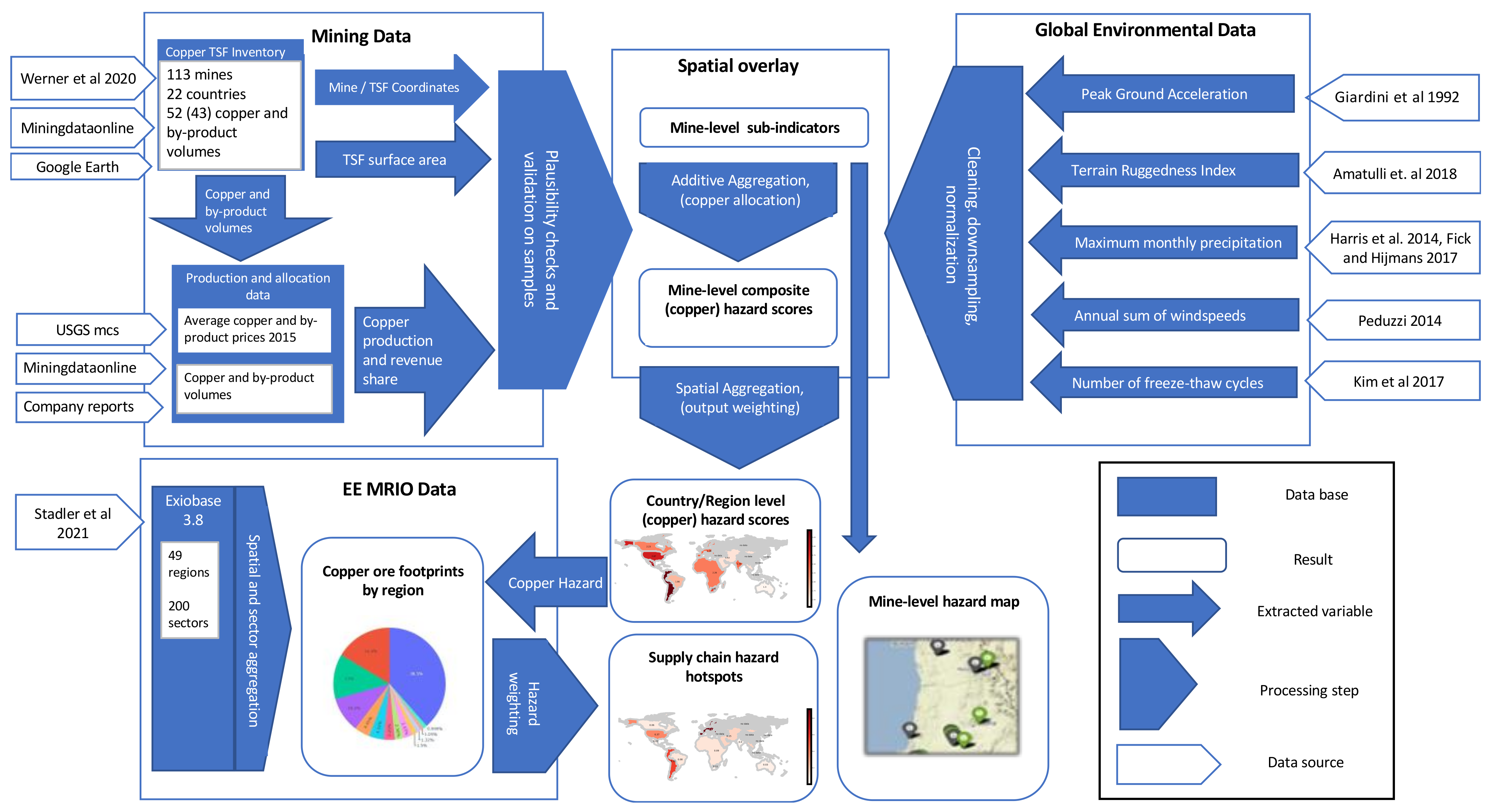
2. Methods and Data

Section 2.1 describes which environmental variables characterizing natural hazards were used (RQ1). Their selection was based on a literature survey of tailings dam failure causes [11,12,38] and previous work concerning quantitative ESG assessment [16,18,39]. Mining data and processing thereof are described in Section 2.2. A composite hazard score was built, aggregated and mapped to answer RQ2 and RQ3. Natural hazards were allocated to copper production and spatially overlaid with TSF coordinates (Section 2.3). Then, consumption-based copper ore footprints were estimated using an MRIO model and supply chain hotspots were identified by weighting ore extraction with regionally aggregated hazard scores (RQ4, Section 2.4). Finally, the effects of different modelling choices and regional differences were examined (Section 2.5). RQ5 was approached in the discussion part. Figure 1 gives an overview of the workflow and data sources.

2.1. Environmental Variables and Composite Indicator Design

Lèbre et al. [39] mapped tailings hazards using a composite score containing seismic activity, terrain ruggedness, precipitation, wind speed and cyclone intensity, all of which have been acknowledged as external factors contributing to tailings dam failures [11,12,50]. Their work served as a basis for this study. Unusual rainfall causing overtopping of TSFs has been identified as the most relevant environmental cause of tailings dam failures [11,12]. Maximum precipitation values from a global time series between the years 2000 and 2018 [46,47] were extracted and used as a proxy.
Seismic activity has been recognized as the second most important environmental cause of tailings dam failures [12]. Here, peak ground acceleration (PGA) values from the global seismic hazard potential map [44] were used. They denote the anticipated maximum ground motion during an earthquake, based on the assessment of previous earthquakes.
High topographic variation contributes to slope instability, erosion and difficult foundation conditions, posing a challenge to tailings dam design [16]. Amatulli et al. [45] used remote sensing data to develop a Terrain Ruggedness Index (TRI), denoting the absolute differences in elevation between a focal cell and its eight surrounding cells. The TRI is provided as summary statistics for spatial grains between 1 km and 100 km. Median values for 10 km grains were chosen.
Tropical cyclones have also contributed to tailings dam failures in the past [39]. Thus, average annual sums of wind speed, based on measurements from official cyclone warning centers and local meteorological agencies [48] entered our model.
Repeated freeze-thaw cycles were experimentally observed to decay the mechanical strength of tailings dams [51] and they have repeatedly been reported as actual causes of tailings dam failures in cold areas [12,52]. Kim et al. [49] used satellite remote sensing to infer information on the earth’s surface freeze-thaw state dynamics. We used their data between the years 2000 and 2017 at a daily resolution for counting the number of transitions between frozen and thawed states. The raw freeze-thaw indicator is the sum of transitions for every grid cell.
TSF size entered the composite indicator as the only man-made hazard. For lack of data on storage volumes, surface area was used as a proxy. Storage volume is well correlated with tailings outflow–runout, on average, amounts to one fifth of the stored tailings volume [11,53]. Concerning likelihood, failures were found to predominantly occur in small to medium-sized TSFs [11,12,38], which suggests that the probability of this hazard to materialize decreases with the size of a TSF. This relationship between probability and hazard was modelled in a first approximation by log-transforming TSF area, which also conforms with the approach used by Kovacs et al. [54]. This way, small TSFs have a relatively high influence compared to large TSFs while maintaining a monotonic relationship between size and hazard.
Prior to aggregation, all hazard variables were normalized to a common scale between zero and one, by replacing each value with its percentile rank. Normalized variables are non-dimensional quantities and are henceforth called ‘sub-indicators’. Applying a generic formula for additive aggregation returns the weighted sum of the six sub-indicators v ^ as a measure of mining hazard MH:
MH = j = 1 6 w j   v ^ j v ^ , w 0 , 1
Bearing in mind the purpose of the indicator as a baseline model, equal weights w were assumed. More sophisticated methods such as participatory weighting require public opinion polls or involvement of experts. Thus, judgement about the relative importance of sub-indicators at a given TSF location was outside the scope of this study and seemed more useful at a later stage of risk assessment.

2.2. Mining Data Selection and Processing

Open data were generally preferred over commercial data for reasons of transparency and reproducibility. To this end, supporting data from recent academic literature on tailings and copper were screened. Werner et al. [40] list coordinates, TSF surface areas, and commodity type as well as main- and by-product volumes for several commodities including 109 entries for copper mines from 23 countries. Their dataset fulfilled all relevant selection criteria and was used as a basis for our analysis.
Data gaps for ore production were filled with figures from Mining Data Online [41] where possible. The remaining gaps were closed using company reports for the year 2015 for consistency with the original data. In twelve cases, where production volumes were not directly reported, they were estimated using ore head grades and recovery rates, nominal production capacities or by extrapolating data from previous years.
Each country’s copper output was compared to the summary figures reported by U.S. Geological Survey [42] and World Mining Data [55]. This was done to ensure that an adequate share of national copper production was covered in the dataset. For countries where only a small fraction of total output was represented, further mines were added after searching the internet and company reports for relevant projects. Table A3 and Table A4 show the outputs of countries and regions that were covered in the dataset after completing this process. Data for China were scarce, covering only six percent of national production, while data for mines in Russia could not be found at all. Both countries were therefore omitted despite being major copper producers. The above treatment yielded a final dataset with n = 112 mines.
Data gaps for TSF surface area were filled by visual inspection and delineation using Google Earth’s measurement tool on images from August 2021 (Figure A3).

2.3. Spatial Overlay and Allocation Model

All environmental variables were obtained as raster data with different granularity. Spatial reference was provided as geographic coordinates in the World Geodetic System 84 (WGS84), where each point denoted the center of a grid cell. For spatial overlay with TSF locations, they were rounded to the first decimal place, resulting duplicate values were averaged and datasets were merged on their coordinates. An accuracy of one decimal place corresponds to a spatial resolution of 11.1 km for both latitude and longitude at the equator [56]. The resolution in longitude is multiplied with the cosine of latitude and hence increases for higher latitudes. Heavy rainfall and earthquakes tend to act on scales of several kilometers while grid cells measured 1 km for rainfall and 10 km for seismicity. Therefore, this accuracy was considered sufficient, bearing in mind both data granularity and the nature of the examined phenomena.
Many copper deposits contain significant amounts of gold, silver, zinc, molybdenum and other by-products [41]. Gold processing, for example, also generates wet tailings which were assumed to equally contribute to TSF size as a hazard component. To avoid a systematic misattribution of hazard to copper supply chains, an allocation model was used. Physical by-product volumes are often several orders of magnitude smaller than those of copper, while their economic value can be four orders of magnitude greater in the case of gold. For this reason, economic allocation was chosen over physical allocation. However, revenues from copper and by-products were found to be mostly reported as summary data for entire company portfolios, unlike physical production volumes, which were often reported on the mine level. Therefore, annual production of copper and by-products was translated into monetary units using global average commodity prices from 2015 [42]. Hazard scores were then attributed to copper according to its share in a mine’s approximated total revenue Ri:
MH Cu , i = j = 1 6 w j v ^ j   R Cu , i R i i = 1 ,   ,   N v ^ 0 , 1 w 1 = w 2 = = 1
where R Cu is the estimated revenue generated from copper production. The approximated revenue of a mine Ri is the sum of known copper and relevant by-product output Pc (including gold, silver, molybdenum, cobalt, nickel and zinc) multiplied with their respective average prices pc as stated in U.S. Geological Survey [42]:
R i = c = 1 7 P c   p c i = 1 ,   ,   N

2.4. Copper Ore Footprints and Supply Chain Hotspots

An Input-Output framework is well suited and often used for large scale environmental footprints [25,26]. It describes the distribution of products in an industry as a set of linear equations which can be used to calculate the entire industrial output needed to satisfy a given final demand. In a multi-regional Input-Output (MRIO) table, national inventories are complemented with bilateral trade data, so it contains an aggregated description of the global economy [25]. The underlying Leontief inverse, also known as the total requirements matrix, is derived from a series expansion of the direct requirements matrix containing the technological coefficients or ‘recipes’ of production:
L = I A 1 = I + A + A 2 + A 3 +
where I is the identity matrix and A is the direct requirements matrix so every power of A represents one tier in the supply chain. L has the dimensions industry by region × product by region. This can be thought of as a multi-index, with each entry denoting an industry or product in a specific region, for example the mining industry in the United States.
Environmental extensions link so-called stressors to the industrial output of a certain industry in a specific region. A well-known environmental stressor is the emission of carbon dioxide into the air. Another such stressor is the domestic extraction of copper ores. Sector-specific, consumption-based, direct and indirect emissions are generally computed as:
b = S Ly ^
where S is the matrix of stressor coefficients with the dimensions environmental stressor × industry by region, L is the Leontief inverse and y the final demand vector of a given region of consumption. The hat symbolizes diagonalization of the product of L and y which is needed to suppress summation over the industry by region dimension of S and L. This way, ore extraction occurring anywhere in the world, driven by direct and indirect copper imports in a given country, was calculated. By linking regional extraction volumes with the respective hazard scores, RQ4, which asks how much tailings-related hazards propagate through a country’s supply chains, could be addressed. An MRIO model does not allow tracing of copper ores back to individual mines, only to the resolution of countries or regions. Still, the chance that copper ore from a specific region was extracted in a particular mine is directly proportional to this mine’s share in the region’s total copper output under the assumption that ore grades and recovery rates are similar within a region. A mine’s hazard score was therefore weighted with its share in copper output upon aggregating hazard to the regional level:
RH Cu = i = 1 n MH Cu , i P Cu , i i = 1 n P Cu , i
where PCu,i stands for the physical production of copper in mine i, n is the number of mines in a given region and MH, RH ∈ [0,6]. The index ‘Cu’ denotes the share of a mine’s total hazard which can be allocated to copper production, as outlined in Section 2.3.
EXIOBASE version 3.8.1 [43] was chosen as an MRIO database for its detailed data on resource extraction, featuring 200 industrial sectors and product groups from 49 regions. Sectors and regions were aggregated into seven summary sectors and eleven regions to facilitate computation as well as meaningful interpretation and visualization of results. Sector and regional aggregation are documented in the Supplementary Materials.
The domestic extraction of copper ores by region was then calculated according to Equation (5), first for the European Union’s final demand, then for the final demand of China, the US, Japan, Germany and India as the world’s five largest economies. The resulting consumption-based copper ore footprints include all copper ores embodied in their supply chains. Finally, hazard hotspots were calculated by weighting the copper ore footprint in each region of ore extraction with its respective regional hazard score:
HFP Cu , i = OFP i i = 1 m OFP i   RH Cu , i
where HFP is the hazard-weighted footprint of a specific region, i.e., a hotspot or ‘coldspot’ in a supply chain, i is the region of ore extraction, m the number of regions of ore extraction in the supply chain of a country, OFP is the demand driven copper ore footprint and RH the regional hazard score.

2.5. Robustness and Uncertainty

Aggregation of sub-indicators can be carried out using additive, geometric or non-compensatory aggregation methods [57,58]. For additive and geometric aggregation, sub-indicators need to fulfil two necessary criteria: first, they are treated as mutually preferentially independent, meaning that they contribute linearly to the composite indicator without interdependencies. Correlation analysis was done in order to check this assumption. Second, aggregation weights are substitution rates rather than coefficients of importance, which means that low scores in one sub-indicator can be at least partially offset by high scores from another [57]. Here, different natural hazards for an individual mine were assumed to both accumulate linearly and substitute for each other. They were added with equal weights in accordance with similar work [54,57,59].
Three different normalization techniques and their effects on both regional scores and relative influence of sub-indicators were compared. Min–Max normalization does not change the shape of the original distribution but it is sensitive to outliers, unlike ranking, which is unaffected by outliers but changes the shape of the original distribution and relative distances between values [58]. In this study, environmental variables could be ranked in two different ways: before and after spatial overlay with TSF data. The first variant computes percentile ranks on the full environmental dataset and then assigns these values to TSF locations. This way, statements about the relative position of a value within the absolute range of all measured values on earth can be made. The second method computes percentile ranks on a subset of the full data, after spatial overlay with TSF locations. Thus, it makes a statement about natural hazards relative to all other TSF locations in the dataset. While neither method allows ad-hoc conclusions about whether a mine is objectively hazardous, pre-overlay ranking contains information about the actual magnitude of a value while post-overlay ranking merely allows for sorting of values within the dataset.
Figure A2 shows histograms of all variables under different ranking and normalization schemes.

3. Results

3.1. Mine-Level Hazard Scores

Hazard scores for the twenty most hazardous mines in the dataset and corresponding raw values of environmental variables are shown in Table 1. Mines from Peru and Chile scored highest in overall hazard: seventeen of the twenty worst-scoring projects are located either in Peru (10) or in Chile (7).
In the full dataset (Table A2), eight mines had a TRI value greater than 45, which is the high-risk threshold defined by Owen et al. [16] while seventeen mines passed their threshold of 3.2 m s 2 for PGA and six mines reached both. Some of the most productive mines were also among the most hazardous, including Escondida, El Teniente, Los Bronces, Collahuasi, Los Pelambres and Las Bambas.

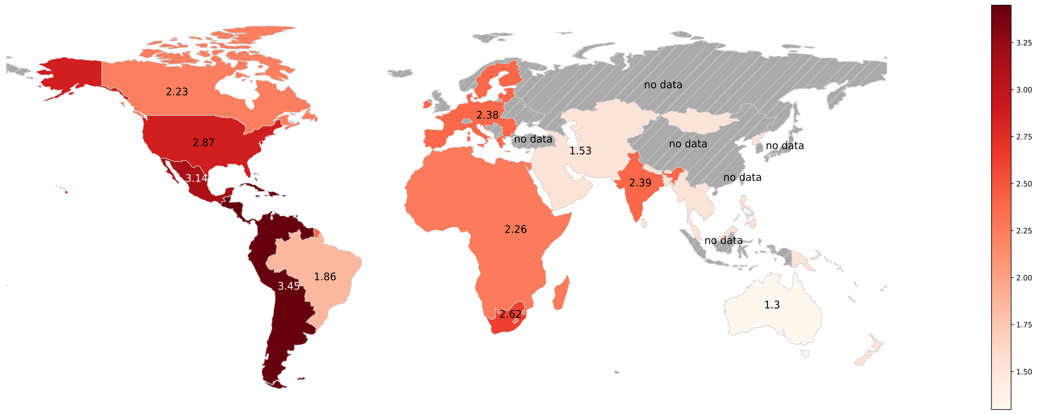
3.2. Regional Hazard Scores

Mine-level results from the previous section were aggregated and output-weighted according to Equation (6). The resulting hazard scores varied between regions (Figure 2). South America and Mexico had the highest average hazard, followed by the United States. Copper mines in Australia scored distinctly lower. The Rest of Asia and Pacific region also scored comparatively low, but data coverage was poor with six mines, covering only 40 percent of the region’s total output (Table A4). Canada, the EU, the Rest of Africa region and India all scored mid-table between 2.23 and 2.39.

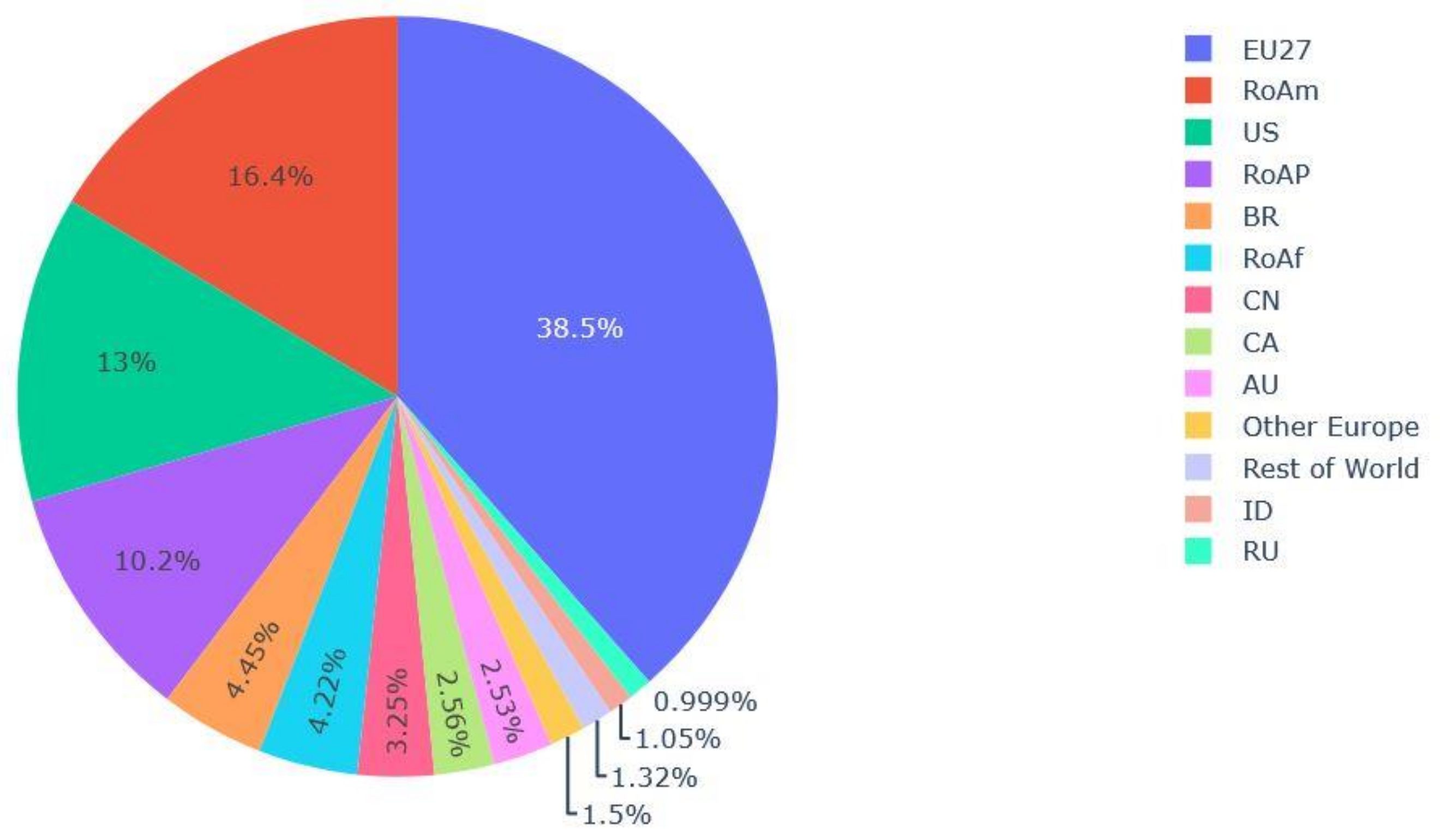
3.3. EU Footprint and Supply Chain Hotspots

The European Union’s copper ore footprint was computed according to Equation (5) and amounts to 151 Mt or 164 Mt depending on the aggregation scheme used (c.f. Discussion); 38.5 percent of embodied copper ores are sourced domestically and another 39.6 percent come from Chile, Peru, the US or the Rest of Asia and Pacific Region (Figure 3).
Weighting the ore footprint with regional hazard scores according to Equation (7), reveals hotspots of tailings-related hazard in Europe’s supply chain (Figure 4). Here, a different picture to the one presented in Figure 2 emerges: copper-related hazard is mainly ‘imported’ from within the EU. Other relevant hotspots are South America and the United States, while almost no copper from Mexico, a high-hazard region, is embodied in European supply chains.

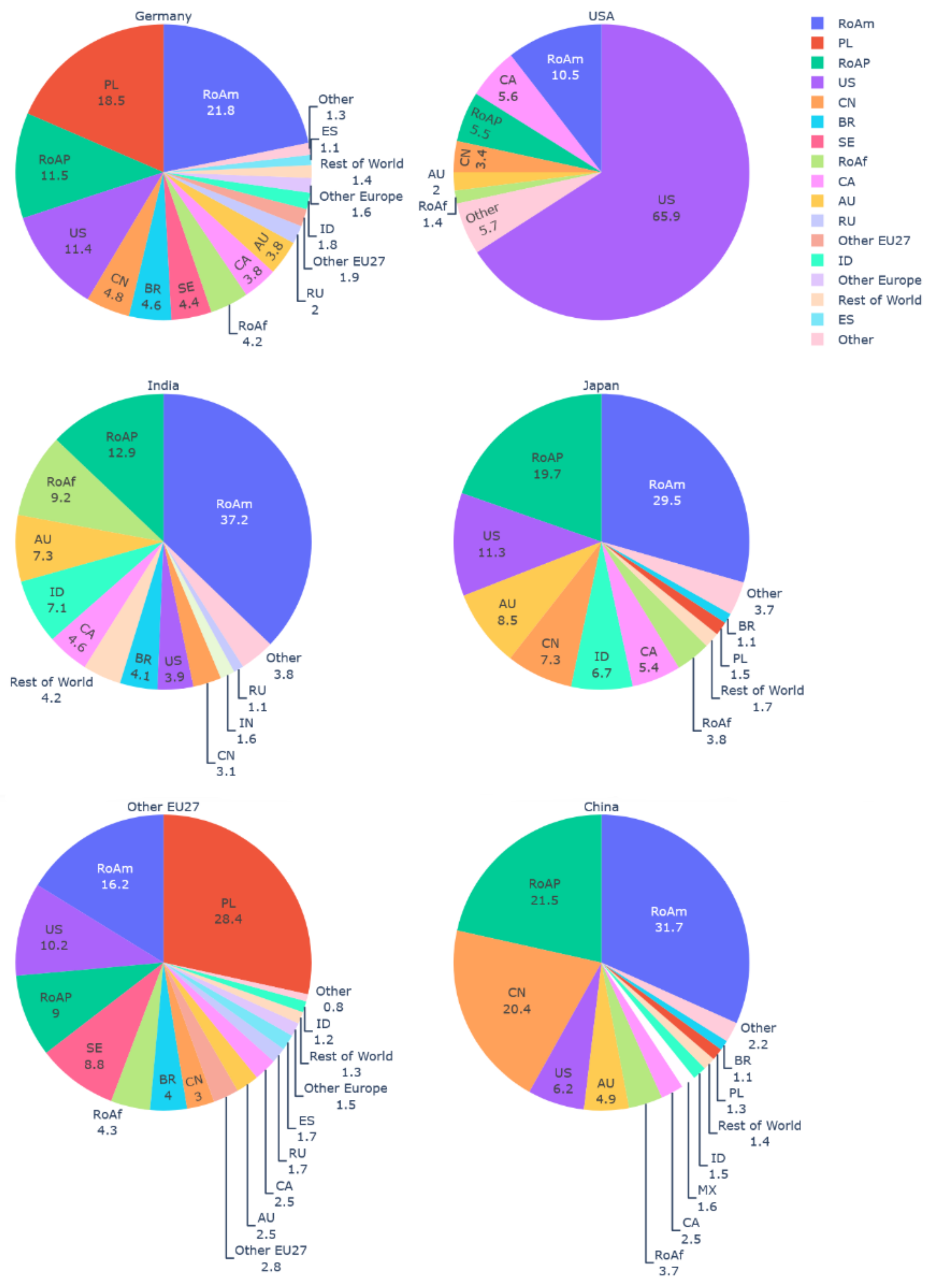
3.4. Footprint Disaggregation and Comparison

For comparison with the European Union, copper ore footprints for the world’s five largest economies were calculated by inserting the respective final demand vectors into Equation (5). Here, the resolution of the MRIO table was set to EU country level to get a more detailed picture (c.f. aggregation table in Supplementary Materials). From this resulted a new table with 25 regions and 16 product groups. The consumption-based footprints are depicted in Figure A1. In 2015, nearly two thirds of copper in US supply chains were supplied by domestic extraction, while India and Japan have little or no national copper resources to extract.
Chile and Peru (RoAm) have substantial shares in every supply chain, between 10.5 percent (US) and 37.2 percent (India). Copper extraction in Poland contributes more than 28 percent to Europe’s supply chain and 18 percent to Germany’s. The Rest of Africa region, including the Democratic Republic of Congo and Zambia as major copper producers, contributes little, usually around four percent, except to the supply chains of India (9 percent).
Total global copper ore extraction in 2015 was around 1.5 Gt, 58 percent of which is embodied in supply chains for the final demand of the world’s five largest economies (China, USA, India, Japan and Germany) (Table 2).
If the remaining EU27 countries are included, two thirds of the world’s copper extraction can be attributed to these six economic entities. To put this number in perspective, these countries also represent nearly half of the world’s population. The annual per capita copper ore footprint was highest in the US with 790 kg, more than twice the values of China and Europe. India’s per capita footprint was around one order of magnitude lower than any of the other national economies under comparison.
An example may illustrate how the findings presented in this chapter can be used to approximately trace ores and hazard to individual mines with little additional information: according to EXIOBASE, about 151 Mt of copper ores were extracted globally in 2015 to satisfy final demand in the European Union, including 28.3 Mt for final demand in Germany (Table 2). About 18.5 percent of the German and 28.4 percent of the remaining EU’s copper ore footprint were sourced in Poland (Figure A1). This amounts to 5.2 Mt of ores for German final demand and 34.7 Mt for the remaining EU. These ores are most likely mined from the Legnica-Glogów copper belt in southwestern Poland where KGHM, Poland’s biggest mining company, operates several large projects [60]. More precisely, 12.7 Mt of ore at a grade of 1.7 percent were extracted at Rudna, 12.4 Mt at 1.7 percent from Polcowice-Sieroszowice and 8.1 Mt at 0.9 percent from Lubin [60]. This yields a theoretical copper output of 499 kt for all three mines, which is roughly in line with the total amount of 426 kt reported by World Mining Data [55], considering recovery rates and losses. The remaining 6.8 Mt of Polish copper ores in Europe’s footprint could either be due to uncertainties in the MRIO table or contributed by other mines if losses at Rudna, Lubin and Polcowice-Sieroszowice were high. Satellite images from Google Earth show that waste from these three facilities is stored at Zelazny Most, Europe’s largest tailings reservoir. Since Poland contributes little to supply chains of other major economies (Figure A1), responsibility for Zelazny Most can be attributed to European countries, both from a producer’s and from a consumer’s perspective. Hazard scores for Zelazny Most were mainly driven by freeze-thaw cycles (Table A1) which should be considered in on-site safety assessments.

3.5. Robustness and Uncertainty

Sensitivity analysis was done for several model configurations prior to computing the final results. The relative influences of different sub-indicators varied across regions (Figure 5a). Precipitation had the highest influence in tropical regions such as Brazil, India and the Rest of Africa. Freeze-thaw cycles contributed little or nothing to the scores of Brazil, India, the Rest of Africa, South Africa and Australia while they had a stronger influence in Canada, the US, Europe, and the Rest of America Region. Cyclones had little or no influence across regions, except for Australia, Mexico and the Asia and Pacific region. Note that especially values for South Africa, India and Brazil are by no means representative of the climate and topography of the entire country since only few mines were contained in the dataset (Table A3).
Correlation analysis was performed to validate the choice of environmental variables used in the composite hazard score (Figure 5b). The values of around 0.5 for earthquakes, terrain ruggedness and freeze-thaw cycles can be explained as follows: 55 mines, 49 percent of the data, are located in the American Cordillera, a chain of mountain ranges including the Andes, the Rocky Mountains and the Sierra Madre in Mexico. They feature a rugged topography (TRI) and high variations in temperature which can cause freeze-thaw events (FT). The American Cordillera is part of the Circum-Pacific-Belt, also known as the Ring of Fire, where the world’s highest seismic activity takes place [61]. An analysis conducted by Lèbre et al. [39] on the full global dataset of TRI and PGA showed that both variables are generally uncorrelated. Their correlations were therefore regarded as a geographic property of the TSF dataset, not as a sign of inherent interdependency. Freeze-thaw cycles may indeed be correlated with TRI for the reason explained above. However, they also occur in flat deserts and generally in regions at high latitude, which is why both variables were kept in the model.
Normalization methods were investigated during the model building process to estimate their effect on final results. Pre-overlay ranking generated the highest scores across all regions, followed by post-overlay ranking (Figure 5c). Min–Max normalization produced distinctly lower scores, often around half the values of pre-overlay ranking. For all three methods, India and Australia had the lowest hazard scores while mines in the Rest of America region scored highest. Wherever a region scored lower than another with one method, this was also true for other methods in most cases with some exceptions: for Min–Max normalization, the Rest of Asia and Pacific region scored distinctly higher than Mexico, Canada, and the US. For pre-overlay ranking, it scored slightly lower than the other three regions and for post-overlay ranking it squared with Mexico but exceeded the US and Canada. Brazil scored lower than the EU27 using pre-overlay ranking but reached higher values for post-overlay ranking and Min–Max normalization.
Tropical cyclone windspeed has a small influence on overall score, irrespective of the normalization method (Figure 5d). TSF size has a disproportionate share of roughly 40 percent when using Min–Max normalization. Pre-overlay ranking puts slightly more emphasis on seismicity (PGA), precipitation (PRE) and terrain ruggedness (TRI) while post-overlay ranking gives more weight to TSF size and cyclone wind speed (CYC). Thus, the influences of sub-indicators are not only a result of their occurrence in the dataset–that is, if more mines are exposed to, e.g., seismic hazard than heavy rainfall–but also of the normalization method used. This is a direct consequence of their altered frequency distributions after normalization (Figure A2).
Ranking was chosen over Min–Max normalization, so scores were not disproportionally influenced by TSF area. Pre-overlay ranking was considered more useful than post-overlay ranking since it contains information about the relative magnitude of a variable compared to all values in the global dataset, not only in relation to other known TSF sites. Further, it allows slightly more influence for seismicity and precipitation, which are the predominant natural causes of dam failures [12].

4. Discussion

4.1. Results

Our method quantified hazards for a global sample of 112 copper mines using five indicators of natural hazards as well as TSF surface area. This way, around two thirds of global copper production were covered and rated. While far from capturing all relevant drivers of actuarial risk, our approach may help to prioritize on-site risk assessments or complement existing efforts by mining companies. The latter are usually narrowly focused on dam stability, so our hazard scores can provide additional context of what Owen et al. [16] call ‘situated risk’. Their study also identified many projects with high ESG risk in Chile, Peru and the USA as opposed to overall low ESG risks in Australia.
Other global-scale, quantitative and transparent risk or hazard assessments of individual mines could not be found in the literature, which was the motivation for constructing an indicator in the first place. However, a dataset compiled by the Global Tailings Review [62] contains qualitative TSF hazard ratings by mining companies, based on the consequences of failure. For 16 of the 25 most hazardous mines identified in our study, additional company ratings were available. They are not directly comparable among each other since different companies used different risk guidelines [62]. A comparison to our hazard score, however, showed that many of the worst-scoring mines also had a high company hazard rating: 15 mines scored either significant, major, high, very high, or extreme. These mines are predominantly located in Chile and Peru including Escondida, Los Bronces, Las Bambas, Los Pelambres, Constancia, Antapaccay, Antamina, and Cerro Verde. Together, they produced around 3 Mt of copper in 2015, 15 percent of the global total. Although disaster prevention should be an end in itself, the possibility of high-consequence failures at any of these mines may also raise concerns about shortages in the global supply network.
MRIO modelling revealed how much copper ore was extracted from which regions to satisfy final demand in the EU, China, India, Japan, Germany, and the USA. This includes direct imports of copper, for example the coils and cables of consumer products as well as embodied copper such the copper inside machinery used to harvest soybeans in Brazil, which are later exported to the EU. However, it does not describe the origin of a particular physical unit of copper. Instead, the likelihood that a unit comes from a particular mine was assumed to be directly proportional to this mine’s share in the national or regional copper output, establishing merely a statistical relation. Weighting the EU’s copper ore footprint with the respective regional hazard scores thus helped to understand through which supply chains tailings-related hazards propagate. Our method showed that Poland is a major hazard hotspot in Europe’s supply chain. In terms of due diligence, this means that European actors seeking to minimize tailings risk in their copper supply chain should look no further than Zelazny Most for a start.
However, the exact origins of raw materials at the first step of supply chains remain difficult to trace, making it impossible to attribute their environmental and social burdens directly to consumers [34]. Gathering and managing the information on global copper production necessary to that end will require substantial work. Our review of available mining data confirms the urgent need for standardized, public and timely risk disclosures which others have demanded already [16,38]. To ensure our material footprint and hotspot approach can eventually be refined with local-scale data, tailings databases should also include production volumes of main and by-products. Until such detailed and up-to-date records are provided, an MRIO analysis disaggregating the copper ore footprint not only by region, but also by product and industry would be a next step to learn more about specific supply chains.

4.2. Model Strengths, Limitations and Uncertainties

Our indicator was designed to capture the most relevant hazards concerning tailings dam failures and used to demonstrate how material footprints can help in tracing this hazard through supply chains. Uncertainty analysis showed that the method employed to normalize variables influences the relative importance of sub-indicators as well as the magnitude of the composite score. Still, the relative positions on the spectrum between low and high hazard remained largely the same between regions across methods. Therefore, absolute scores have little practical use, while they help to compare hazards from different mines and regions on a global scale. Condensing a complex phenomenon into a one-dimensional number naturally bears the risk of oversimplification and misinterpretation. However, a composite score including several dimensions of hazard was considered more helpful for hotspot screening than using a highly disaggregated footprint for every sub-indicator. We preserve and report the individual components of our composite hazard score to allow for scientific scrutiny. Transparent and detailed data on individual hazards are needed to enable different weighting schemes and to allow for an overlap with mine-specific impact estimates, such as earthquake or rainfall simulations.
While Owen et al. [16] covered a broader set of ESG variables and risk dimensions, they used conservative parameters such as project age and thresholds in a multi-level selection process to narrow down their global sample of mines. This allowed proceeding to local-scale GIS analysis for exposure and vulnerability assessment. Our approach, on the other hand, aimed to keep the sample as large, unbiased and transparent as possible as a first step towards a back-end database containing raw data relevant for risk assessment. So far, it fails to capture the intricate factors that determine the actual risk level of a project, including exposure and vulnerability of people and the environment.
Dam failures constitute a major hazard in mining, yet a low failure risk must not be mistaken for generally safe mining practices. There are many other concerns, such as landslides, land grabbing or chronic pollution by seepage of toxic waste. A low ranking on the tailings hazard score does not, therefore, imply that a mine is safe for workers, host communities or the environment. Conversely, a high score does not allow the assertion that a project is particularly risky, but merely suggests that a mine is located in an area featuring potentially detrimental environmental factors concerning dam failure.
Some major copper producers are not represented in the dataset. Mines from China, Russia and Indonesia are entirely missing, even though these countries produced 1710 kt, 732 kt and 587 kt of copper in 2015, respectively [42,55]. Kazakhstan produced around 468 kt of copper in 2015 [55], but only Orlovsky mine with a production of 254 kt was included in the dataset. Consequently, hazard scores for copper from the Asia and Pacific region in the current analysis are not useful. With the remaining data, tailings hazard accompanying two thirds of the world’s copper production could be quantified. South Africa, Mexico and the Rest of Africa region had the poorest coverage, while copper from the USA, Australia, Canada and the Rest of America region was well captured, increasing the robustness of the hazard estimates for these regions. Copper ore footprints, on the other hand, were computed directly from the MRIO table (including entries for China, Russia and Indonesia). They are robust within the uncertainty range of EXIOBASE 3.8, which will be discussed below.
Our analysis depicts a snapshot of the years 2013 or 2015 for MRIO data and production volumes of mines, respectively. Since then, the copper landscape has changed; Kazakhstan, for example has increased its copper production by 20 to 30 percent [55,63] and the Dem. Rep. Congo has recently started the high-grade Kamoa-Kakula project. With an estimated average annual production of almost 1 Mt of concentrated copper, it would become the world’s second largest copper mine [41].
Mines tend to be less efficient towards the end of their life cycle when high ore grades have already been extracted. This often results in over-proportional growth of TSFs which was not anticipated in the planning and approval process, so old mines can pose a particularly high risk [38]. To reflect this in the footprints, a life cycle perspective on tailings risk could be incorporated by linking MRIO time series with mining data and integrating ore footprints and production volumes over time. Finally, climate models should be taken into account when quantifying natural hazards with respect to the future, as demonstrated in [64].
It is important to note the consequences of applying different aggregation schemes to the MRIO table: using the original 11 regions × 7 products MRIO table, the EU’s copper ore footprint was 164 Mt, while using the disaggregated 25 regions × 16 products table yielded 151 Mt, a difference of eight percent. Koning et al. [65] quantified errors in the material footprints of countries when resolving the product dimension of EXIOBASE from 200 to 60 products. They found percentage changes between −29 and +14 percent. The same study showed that spatial aggregation from 48 countries to four regions changes the results for material footprints by between −2.7 and +2.1 percent. Therefore, it is generally advisable to calculate emissions with a disaggregated background MRIO table first and then aggregate the results for meaningful interpretation and display [65,66].
Giljum et al. [67] investigate deviations between three different MRIO databases (EXIOBASE, Eora, ICIO) and their effects on material footprints. They find the footprints for China, USA, India and Germany to be insensitive to the MRIO table used, while Japan’s material footprint was 12 t per capita when calculated with EXIOBASE, 19 t using ICIO and 20 t when calculated with Eora. Therefore, Japan’s copper ore footprint is likely to be underestimated in this study, explaining its distinctly lower value.
Wiedmann et al. [68] also compare the overall material use of nations and find that China has the largest footprint, followed by the USA, Japan and India. According to their study, the United States’ per capita material footprint was around 28 t, whereas people in India use on average 3.7 t of materials per year. This difference is bigger for copper, where the USA’s footprint is 25 times larger than India’s, and can be explained by the technology-intensive lifestyle in high-income countries.
Setting aside the case of Japan, the differences between countries seem realistic considering their GDP and average material standard of living. Still, a disaggregated, sector-specific analysis would be interesting as well as a breakdown by production, imports, and exports. Comparing footprints from other major economies would also help to see a more complete picture.

4.3. Policy Relevance and Future Research

From a due diligence perspective, withdrawing from risk hotspots would be a poor strategy for several reasons: first, there is currently no way of replacing major copper producers such as Chile and Peru in the global supply network, not to mention the potentially devastating effects on their economies. Copper deposits are immobile assets that cannot be mined elsewhere, and mining projects are planned with long time horizons. Secondly, withdrawal would not at all address the necessity of mitigating tailings risk from existing or new tailing deposits.
Instead, the basis for a new tailings risk policy should be to close the knowledge gaps with publicly available risk assessments including on-site dam inspections as well as broader and transparent ESG considerations. From there, a prioritization scheme could be set up, directing investments into risk mitigation to those mines and communities where it is needed most urgently. Following the footprint logic, a share of these costs must be ascribed to consumers.
To this end, a global fund could be installed into which countries and companies pay according to their ore footprint or imported tailings risk. Investments from this fund would be directed to support mine operators and regulators in establishing and enforcing best practices for tailings management. Country-scale solutions would need to be based on voluntary international agreements while industry behavior can be stirred with national due diligence laws.
The general problem of assigning responsibility for environmental impacts is not new, but is still actively discussed in the literature [23,28,69,70,71]. Traditionally, production-based accounts as required by the United Nations Framework Convention on Climate Change (UNFCCC) and reported by the IPCC quantify impacts within geographic boundaries. Many have argued that this often results in unfair national emission inventories for countries with a low standard of living producing goods mostly intended for export [28,70,71]. Besides, asymmetrical policies between countries can cause leakage effects such as outsourcing of emission-intensive industries [72]. In the case of tailings risk, leakage should be less relevant since raw material extraction is mainly determined by geological factors, while fairness remains a central and unresolved issue.
Consumption-based models, on the other hand, account for international trade, allocating environmental burden entirely to the final demand in that country where a product or service is consumed [28]. It increases fairness compared to production-based accounts, considering that consumption and wealth in the industrialized world are the main drivers of environmental pressure [70].
On the downside, consumption-based accounting can mute incentives for cleaner production in producing countries since the environmental ‘bill’ is assigned entirely to consumers [71]. Besides, Peters [28] argues that production-based accounting is more likely to be taken up by policy makers considering its lower uncertainty, established reporting and consistency with political and local environmental boundaries.
Attempting to consolidate both approaches, Lenzen et al. [70], developed a concept of shared responsibility assigning weights to national emission inventories derived from value added along the supply chain. Bastianoni et al. [71,72,73,74] propose a similar, hybrid approach of dividing the supply chain into multiple producer–consumer tiers and assigning responsibility based on the carbon emissions added. Piñero et al. [23] compare the value-added approach to producer, consumer and income responsibility for material footprints. They argue that a shared responsibility model could be perceived as fairer and thus receive better support from actors strongly affected by either of the full allocation approaches. A shared responsibility model mapping both value-added and economic externalities such as tailings risk in material supply chains should be investigated in future work.

5. Conclusions

Our research adds a new angle to the discussion about tailings risk by estimating copper ore footprints and tailings-related hazard hotspots for the European Union and five major economies. A unique and transparent indicator of tailings hazard was developed and applied to a global dataset of copper mines. The results are not definitive but rather represent a step towards holistic tailings management. Building on our work and the findings of others, researchers may soon make an educated guess about which tailings storage facilities are most likely to fail next. Meanwhile, mining corporations must immediately begin to increase transparency, encourage independent assessments and mitigate risks. Eventually, this could lead to a change of perception of tailings disasters, shifting from the occasional misfortune to a severe yet preventable systemic risk.
The strength of the footprint approach is to reveal and quantify the environmental impacts associated with human consumption. We showed how, as in the case of Poland, regionally coarse footprint data can be refined with readily available, mine-level production data. This sheds light on the specific origins of copper embodied in Europe’s supply chain with little additional information required. However, this heuristic approach will not be applicable as easily for other regions where production is spread across a larger portfolio of mines and whose copper is exported to a variety of countries.
There is currently no such thing as safe mining and raw materials are embodied in virtually every supply chain. Therefore, withdrawal from certain risk hotspots alone will neither work in practice nor acknowledge the existing legacy of tailings ponds. Instead, joint efforts could help to direct financial means and expertise to where they are needed most urgently for risk mitigation. New risk policies and mitigation strategies should consider a shared responsibility approach, dividing the costs between both producers and consumers.

Supplementary Materials

The following supporting information can be downloaded at: https://www.mdpi.com/article/10.3390/resources11100095/s1, Table S1: Tailings data; Table S2: Sector_aggregation; Table S3: Master_v2.

Author Contributions

Conceptualization, S.L.N. and S.P.; methodology, S.L.N.; software, S.L.N. and S.P.; investigation, S.L.N.; resources, S.P.; data curation, S.L.N. and S.P.; writing—original draft preparation, S.L.N.; writing—review and editing, S.P.; visualization, S.L.N.; supervision, S.P. All authors have read and agreed to the published version of the manuscript.

Funding

This research received no external funding.

Data Availability Statement

Publicly available datasets were analyzed in this study. This data can be found under the following URLs: Seismic hazard data: http://gmo.gfz-potsdam.de/pub/download_data/download_data_frame.html (accessed on 16 October 2022); Precipitation data: https://www.worldclim.org/data/monthlywth.html (accessed on 16 October 2022); Terrain Ruggedness: https://www.earthenv.org/topography (accessed on 16 October 2022); Cyclone Data: https://wesr.unepgrid.ch/?project=MX-XVK-HPH-OGN-HVE-GGN&language=en (accessed on 16 October 2022); Freeze thaw cycles: https://nsidc.org/data/NSIDC-0477 (accessed on 16 October 2022); Raw material output of countries: https://www.world-mining-data.info/?World_Mining_Data___Data_Section (accessed on 16 October 2022).

Acknowledgments

We thank Nikolaus Geiler for sharing his expertise on water policy and his guidance throughout the project.

Conflicts of Interest

The authors declare no conflict of interest.

Appendix A

Figure A1. Consumption-based copper footprints of the world’s five largest economies and the EU27 by region of ore extraction for the year 2015. Countries and regions that contributed less than one percent to the footprint were aggregated for better readability. Mass-based, not hazard-weighted.
Resources 11 00095 g0a1
Figure A2. Frequency distributions of raw environmental variables, pre-overlay rank and Min–Max scaled sub-indicators. Post-overlay ranking yields uniform distributions for all sub-indicators and is therefore not shown.
Resources 11 00095 g0a2
Figure A3. (a) Cairn Hill mine, Australia: No TSF was visible on satellite imagery. Dry stacking of tailings was assumed, and the mine was omitted from the dataset since only wet tailings were considered relevant for dam failures. (b) Presumably shared TSF between Chuquicamata, Radomiro Tomic and Ministro Hales mines in Chile. The measured surface area of 66.5 km2 was split according to the relative copper output of each mine. Vice versa, in cases where multiple TSFs belonged to a single mine, their surface areas were added. The image also illustrates how TSF boundaries could not always be clearly distinguished. Areas which looked as if they had run dry (dark brown) were not included. Differences to TSF areas from 2015 reported by Werner et al. [40] were found to be small and therefore acceptable.; Images: Google, © 2022 Maxar Technologies, CNES/Ai.rbus.
Resources 11 00095 g0a3
Table A1. Mine-level results. For an explanation of acronyms and variables refer to Table 1 in the main part.
MineCountryRegionCopper Production [kt]Overall HazardCopper-Related HazardPGATRIPRECYCFTTSF Area
El TenienteChileRoAm471.164.734.413.4747.69499.810.002076.017.0
ToromochoPeruRoAm182.294.314.313.8549.061700.150.002164.02.3
AntaminaPeruRoAm107.704.293.253.2342.81699.670.001359.65.1
Las BambasPeruRoAm453.754.193.782.2440.75412.310.002848.52.6
PadcalPhilippinesRoAP17.244.164.163.1571.75807.06329.000.01.6
Bingham CanyonUSAUS92.024.162.651.9034.31133.700.001643.131.8
ConstanciaPeruRoAm105.904.153.812.1730.59439.260.003396.02.5
YauliPeruRoAm2.504.150.123.6845.691686.550.002260.01.1
AndinaChileRoAm224.264.123.854.264.25298.150.001537.819.2
Marcapunta NortePeruRoAm32.064.023.503.345.751166.210.002347.72.7
El SoldadoChileRoAm36.003.973.974.6765.88284.730.001537.81.8
Tintaya/AntapaccayPeruRoAm202.103.963.452.1413.88379.200.003350.02.3
MorocochaPeruRoAm8.163.881.593.7641.191637.930.002164.00.1
Los BroncesChileRoAm401.703.883.883.7190.31231.410.002228.01.0
ToquepalaPeruRoAm143.003.833.832.9240.75225.440.00516.514.5
Cerro CoronaPeruRoAm30.043.821.763.3239.75545.710.001022.01.0
EscondidaChileRoAm1226.503.703.613.0012.135.820.002594.450.7
Los PelambresChileRoAm363.203.673.333.6657.19179.920.002093.20.5
CollahuasiChileRoAm433.103.673.522.4425.5695.060.001508.714.4
Highland ValleyCanadaCA151.403.573.310.8515.6190.130.001211.021.6
Carmen de AndacolloChileRoAm68.303.533.074.2628.38108.870.001384.52.6
Toledo-Carmen/LutopanPhilippinesRoAP34.213.423.042.3330.00394.0832.500.01.1
Boddington+HedgesAustraliaAU37.993.380.621.008.13238.891.00201.916.4
Radomiro TomicChileRoAm315.753.333.302.6517.3119.990.00945.824.3
Cerro VerdePeruRoAm199.363.323.323.4128.5673.790.001361.44.0
ChuquicamataChileRoAm308.633.322.802.6517.3119.990.00945.823.8
GibraltarCanadaCA63.963.303.300.6212.94106.460.001154.08.1
Ministro HalesChileRoAm238.313.302.962.6517.3119.990.00945.818.4
HuckleberryCanadaCA19.633.283.070.4526.63234.340.001319.71.4
Phoenix (mill+heap leach)USAUS21.003.281.141.7315.1960.940.001818.03.0
RobinsonUSAUS57.003.282.490.8714.8163.420.001610.06.6
Buenavista (Cananea)MexicoMX284.003.273.180.1717.00340.310.00242.117.7
Copper Mountain (Similkameen)CanadaCA35.383.272.771.1529.38136.790.001336.01.4
La CaridadMexicoMX131.003.273.240.2726.81307.430.0076.416.7
Mount PolleyCanadaCA3.633.221.690.6219.13141.660.001285.32.2
PunitaquiChileRoAm8.163.203.204.4437.13135.720.001287.50.2
Cadia GroupAustraliaAU73.703.201.090.9013.56210.320.00343.68.0
BagdadUSAUS95.253.183.180.7127.38125.430.00647.97.4
Rudna Polkowice LudinPolandEU27499.603.142.570.234.19170.230.00972.912.5
MorenciUSAUS480.813.123.120.6316.94113.580.00778.37.8
BolivarMexicoMX9.983.103.100.7351.97402.922.83280.00.1
SudburyCanadaCA98.003.101.410.322.81169.171.001343.47.8
CuajonePeruRoAm178.003.073.072.8944.09247.000.00516.50.3
KansanshiZambiaRoAf226.673.052.710.755.88431.010.000.012.8
Centinela (mill+heap leach)ChileRoAm145.203.032.412.886.387.110.00995.19.9
LumwanaZambiaRoAf130.183.033.030.727.63396.920.000.011.0
Duck PondCanadaCA6.103.002.140.334.75199.2016.11910.00.9
Pinto ValleyUSAUS60.332.992.940.6830.44167.490.00158.54.8
Bajo de la Alumbrera-Bajo el DuraznoArgentinaRoAm61.802.991.831.7920.2581.960.00536.05.4
TelferAustraliaAU23.122.990.521.021.75243.7768.130.05.0
Phu KhamLaosRoAP71.162.982.450.8841.94786.000.000.01.6
Mount MilliganCanadaCA32.212.971.410.3111.59110.110.001196.73.3
Kamoto GroupDem. Rep. CongoRoAf147.772.941.950.525.25340.670.000.017.5
Mount CarltonAustraliaAU1.142.890.150.9216.38458.9210.500.00.3
NchangaZambiaRoAf24.372.852.850.354.63476.830.000.012.7
Sierra GordaChileRoAm87.002.842.363.064.254.930.00995.17.3
AitikSwedenEU2767.132.831.960.264.06122.450.00749.112.0
ContinentalUSAUS31.752.832.830.5532.25169.190.00774.70.4
Mopani (Nkana+ Mufulira)ZambiaRoAf92.002.812.810.224.63486.790.000.014.5
MissionUSAUS68.302.812.810.554.88199.320.0099.09.6
SierritaUSAUS85.732.802.800.524.06193.710.00161.511.2
Mount IsaAustraliaAU86.612.790.740.374.94434.580.000.010.1
Kidd CreekCanadaCA40.102.791.620.381.38173.600.00784.612.6
Afton+New AftonCanadaCA39.012.791.750.6721.8873.290.001367.50.8
Candelaria-Ojos del SoldadoChileRoAm144.832.782.454.0826.1613.200.00351.04.4
ZaldivarChileRoAm98.882.772.772.9613.885.890.002594.40.2
PalaboraSouth AfricaZA49.102.752.630.116.81224.010.007.517.0
Trident-SentinelZambiaRoAf32.972.742.740.733.13351.230.000.010.7
La RondeCanadaCA4.942.740.210.494.25162.250.00835.52.1
KonkolaZambiaRoAf40.222.702.700.483.25463.590.000.08.9
Cerro ColoradoChileRoAm99.842.692.692.8214.4432.510.001841.50.1
El ChinoUSAUS142.432.672.670.532.88126.610.00774.75.2
Boliden AreaSwedenEU273.852.670.190.234.00128.630.00798.55.0
Boss Mining Group (Kakanda-Luita-Lubumbashi)Dem. Rep. CongoRoAf75.502.672.670.7612.19371.560.000.01.9
Tenke FungurumeDem. Rep. CongoRoAf203.962.671.900.7011.63368.700.000.02.1
RayUSAUS75.002.652.650.6618.25111.050.00158.54.1
Voisey’s bayCanadaCA32.002.640.580.316.66122.530.00771.92.9
MutandaDem. Rep. CongoRoAf216.002.631.900.685.50349.210.000.03.5
SeponLaosRoAP89.252.602.600.3814.86744.621.000.00.6
El SalvadorChileRoAm48.582.562.563.6214.388.360.001615.00.1
SossegoBrazilBR104.002.552.200.0118.31444.580.000.07.9
Neves CorvoPortugalEU2755.832.511.701.194.56261.770.004.41.8
Oyu TolgoiMongoliaRoAP202.202.440.100.691.8151.190.001135.84.2
MintoCanadaCA16.522.432.000.5517.0090.580.00840.00.2
MalanjkhandIndiaIN26.202.432.430.144.63742.710.000.03.0
SaloboBrazilBR155.002.361.710.0120.22385.540.000.04.1
FrontierDem. Rep. CongoRoAf65.882.362.360.233.13467.340.000.03.7
ManitobaCanadaCA41.382.341.000.004.13150.510.00785.84.7
ChapadaBrazilBR59.422.331.670.016.25397.000.000.08.8
Las CrucesSpainEU2770.032.322.320.955.44257.190.0024.70.3
CozaminMexicoMX15.652.301.660.468.19179.911.0177.00.3
Mantos BlancosChileRoAm53.502.262.263.579.880.000.00195.51.5
NorthparkesAustraliaAU49.962.211.870.811.63137.510.00332.13.0
Silver BellUSAUS19.002.172.170.564.88115.880.0017.72.4
KanmantooAustraliaAU17.312.131.940.909.13111.500.0089.40.4
RuashiDem. Rep. CongoRoAf35.062.131.330.722.63420.270.000.00.8
PyhäsalmiFinlandEU2712.052.091.290.192.50137.780.00646.41.4
EtoileDem. Rep. CongoRoAf25.002.061.460.722.63420.270.000.00.3
KinsevereDem. Rep. CongoRoAf80.172.042.040.762.00411.110.000.00.7
Khetri GroupIndiaIN2.332.042.040.651.38313.540.004.01.4
Ernest HenryAustraliaAU70.731.991.570.270.63437.960.000.03.9
Chibuluma SouthZambiaRoAf12.731.951.950.263.50489.320.000.00.3
Olympic DamAustraliaAU124.501.921.610.901.3877.470.003.06.6
Golden GroveAustraliaAU25.601.830.891.011.88101.902.001.60.5
OsborneAustraliaAU19.301.831.440.341.50246.910.003.01.3
OrlovskyKazakhstanRoAP254.001.771.660.341.00106.330.00614.11.6
TrittonAustraliaAU30.251.751.750.511.88122.890.0027.41.4
Cobar-CSAAustraliaAU48.661.671.620.392.00106.070.003.92.0
Prominent HillAustraliaAU130.311.621.350.641.3877.300.004.02.4
PeakAustraliaAU6.351.570.390.412.00103.330.0038.70.9
De GrussaAustraliaAU70.021.421.130.580.75153.951.000.00.3
Guelb MoghreinMauritaniaRoAf45.001.070.830.150.8866.940.000.02.1
Table A2. Literature survey of previous work on quantitative ESG risk assessment in the context of mining. The table is not exhaustive but aims to capture recent and relevant contributions on which this study was built.
PublicationESG DimensionsRisk DimensionsIndicatorsScaleTailings Specific 1Resource Focus
Miranda et al. (2003)E, S, G 2Natural hazard, Vulnerability 3 Protected areas, areas of high conservation value, intactness of ecosystems, (ground)water availability, seismic hazard, chemical weathering, Capacity for informed decision making, construction standards for mine structures, Voice and accountability, corruption, political stability, government effectiveness, rule of law, type of operation, waste disposal methodCoarse,
Global & local
(US, Papua New Guinea, Phillipines)
noHardrock mining (metals and precious gemstones)
Kovacs and Lehunova (2020)E, SNatural and man-made hazards, exposureTailings capacity, tailings toxicity, seismic hazard, flood hazard, activity status/management conditions, dam factor of safety, human population exposure, potentially exposed waterwaysRegional (Danube river basin), nationalyesunspecific
Owen et al. (2019)E, S, GNatural hazards, vulnerability, exposureSeismic hazard, terrain ruggedness
index, aqueduct water risk, key biodiversity areas
World Database on protected areas, Human Footprint, Indigenous Peoples Land, Fragile State Index, Resource Governance
Index, Policy Perception Index, Ease of Doing Business Index
Global → localyesGold, copper, iron, bauxite
Newland Bowker (2021)GMan-made hazardsHost country failure history (%worldwide failures/%world mineral production), tailings capacity, activity status/management conditions, facility age, design typeglobalyesunspecific
Luckeneder et al. (2021)EVulnerability, exposureSpecies richness, protected areas, available water remaining index (AWaRe),Global, fine grainednobauxite, copper, gold, iron, lead, manganese, nickel, silver and zinc
Lebre et al. (2019)E, S, GNatural hazards, vulnerability, exposureSame as Owen et al. (2019)globalnoIron, copper, aluminium
Lebre et al. (2020)E, S, GNatural hazards, vulnerability, exposureSeismic risk, average wind speed, terrain ruggedness, cyclone risk, maximum annual precipitation, baseline water stress, inter-annual water variability, Key Biodiversity areas, Biodiversity Hotspots maps, Total Species Richness maps, Global human settlement, population density in 100km radius, indigenous peoples map, global farmland and pastures map, forest extent map, Human Development index, Gini coefficient, Total dependency ratio, Worlwide Governance Indicators (World Bank)globalnoEnergy transition metals, including iron, copper, aluminium, nickel, lithium, cobalt, platinum, silver, rare earths
Northey et al. (2017)ENatural hazards (water risk), vulnerabilityWater criticality (CRIT), supply risk (SR), vulnerability to supply restrictions (VSR), environmental implications (EI) of water use, watershed or sub-basin scale data for blue water scarcity (BWS), water stress index (WSI), available water remaining (AWaRe), basin internal evaporation, recycling (BIER) ratios, water depletion index (WDI)globalnoCopper, lead-zinc, nickle
1 Indicates whether the study was particularly concerned with tailings risks as opposed to a broader view incorporating other risks and detriments associated with mining, such as freshwater depletion or habitat fragmentation by mining infrastructure. 2 The authors acknowledge limitations due to lack of data and fuzziness of concepts especially in the governance dimension, which results in different subsets of indicators for different countries, limiting their comparability. 3 Here defined as: the likelihood of destruction or degradation arising from a natural or environmental hazard, such as destruction of an intact ecosystem or damages to an aquatic system from water pollution.
Table A3. Cumulative copper production for the year 2015, by country in thousand metric tons. Percentages of national production were derived from values reported by World Mining Data (2021) and USGS (2017). Peru’s portfolio was extended by the Las Bambas project, which started production in late 2015, with data from 2017 (453 kt) to obtain a more realistic representation of the country’s situation. A coverage of 100 percent was hardly possible since only copper mines producing wet tailings were considered. This way, copper produced by solvent extraction and electrowinning as well as by-product copper was excluded.
CountryTotal ProductionDataset
n MinesProductionPercent of Total
Chile576019477382.9
China17103112.96.6
Peru1700 (+453)121644.976.4
USA1380121228.689
Dem. Rep. Congo10208849.383.2
Australia97116815.584
Russia732000
Zambia7127559.178.5
Canada69714584.383.8
Mexico5944440.674.2
South Africa77149.163.8
Brazil351331890.6
India34228.583.3
Poland4261499 1117.2
Argentina62162100
Finland4211228.5
Spain13017053.8
Laos1682160.495.5
Mauritania45145100
Mongolia336120260.1
Philippines84251.461.1
Portugal83155.867.2
Kazakhstan468125454.2
Other1818
World19100 (+453)115(−3)12,77565.3
1 Number estimated using ore grades and ore volume as reported in KGHM (2015), excluding losses.
Table A4. Copper production by region for the year 2015 in thousands of metric tons. Data resolution in EXIOBASE 3.8 differs between world regions: while each country in the European Union represents an entity of its own, South America is divided into Brazil and all other countries. In contrast, the mining dataset contained only six mines from five countries within the European Union but 19 mines from Chile and 12 from Peru. To account for this imbalance, regional aggregation was done using the following scheme: countries remained a unique entity when sufficient copper data as well as Input–Output data were available. This applied to Australia, Canada, USA, Mexico, Brazil, India and South Africa. Whenever copper data were available while Input–Output data were not, countries were aggregated into regions. This was the case for Chile, Peru, Argentina, Dem. Rep. Congo, Zambia, Laos, Philippines, Kazakhstan, Mauritania, and Mongolia. They were aggregated into Rest of South America, Rest of Africa and Rest of Asia and Pacific respectively. Since no copper data were available for most European countries, all EU27 countries were initially regarded as an economic entity and aggregated as EU27. Later, European copper producers were disaggregated from the EU27 region to further refine the picture. Percentages of regional production were derived from the values reported by World Mining Data [55] and U.S. Geological Survey [42]. A coverage of 100 percent was hardly possible since only copper mines producing wet tailings were considered. This way, copper produced by solvent extraction and electrowinning as well as by-product copper was excluded.
EXIOBASE RegionTotal ProductionDataset
n MinesProductionPercent
Rest of America7556.932648085.7
Rest of Africa1945.216145374.7
Australia97116815.583.9
Canada69714584.383.8
USA138012122989.1
EU27878.26708.580.7
Rest of Asia & Pacific1652666840.4
Mexico5944440.674.2
Brazil3513318.490.7
India34.2228.583.3
South Africa77149.163.8

References

  1. International Resource Panel. Global Resources Outlook 2019: Natural Resources for the Future We Want. 2019. Available online: https://www.resourcepanel.org/reports/global-resources-outlook (accessed on 17 September 2022).
  2. Luckeneder, S.; Giljum, S.; Schaffartzik, A.; Maus, V.; Tost, M. Surge in global metal mining threatens vulnerable ecosystems. Glob. Environ. Change 2021, 69, 102303. [Google Scholar] [CrossRef]
  3. Lèbre, É.; Owen, J.R.; Corder, G.D.; Kemp, D.; Stringer, M.; Valenta, R.K. Source Risks As Constraints to Future Metal Supply. Environ. Sci. Technol. 2019, 53, 10571–10579. [Google Scholar] [CrossRef] [PubMed]
  4. Calvo, G.; Mudd, G.; Valero, A.; Valero, A. Decreasing Ore Grades in Global Metallic Mining: A Theoretical Issue or a Global Reality? Resources 2016, 5, 36. [Google Scholar] [CrossRef] [Green Version]
  5. Bowker, L.; Chambers, D. In the Dark Shadow of the Supercycle Tailings Failure Risk & Public Liability Reach All Time Highs. Environments 2017, 4, 75. [Google Scholar] [CrossRef] [Green Version]
  6. Northey, S.; Mohr, S.; Mudd, G.M.; Weng, Z.; Giurco, D. Modelling future copper ore grade decline based on a detailed assessment of copper resources and mining. Resour. Conserv. Recycl. 2014, 83, 190–201. [Google Scholar] [CrossRef]
  7. Mudd, G.M.; Weng, Z.; Jowitt, S.M. A Detailed Assessment of Global Cu Resource Trends and Endowments. Econ. Geol. 2013, 108, 1163–1183. [Google Scholar] [CrossRef]
  8. ICOLD. Tailings Dams Risk of Dangerous Occurrences: Lessons Learnt from Practical Experience; Bulletin 121; International Commission on Large Dams (ICOLD): Paris, France, 2001. [Google Scholar]
  9. Roche, C.; Thygesen, K.; Baker, E. Mine Tailings Storage: Safety Is No Accident: A UNEP Rapid Response Assessment. Nairobi and Arendal. 2017. Available online: www.grida.no (accessed on 22 September 2022).
  10. Silva Rotta, L.H.; Alcântara, E.; Park, E.; Negri, R.G.; Lin, Y.N.; Bernardo, N.; Mendes, T.S.G.; Souza Filho, C.R. The 2019 Brumadinho tailings dam collapse: Possible cause and impacts of the worst human and environmental disaster in Brazil. Int. J. Appl. Earth Obs. Geoinf. 2020, 90, 102119. [Google Scholar] [CrossRef]
  11. Azam, S.; Li, Q. Tailings Dam Failures: A Review of the Last 100 years. Geotech. News 2010, 28, 50–54. [Google Scholar]
  12. Rico, M.; Benito, G.; Salgueiro, A.R.; Díez-Herrero, A.; Pereira, H.G. Reported tailings dam failures. A review of the European incidents in the worldwide context. J. Hazard. Mater. 2008, 152, 846–852. [Google Scholar] [CrossRef] [Green Version]
  13. ICMM. Mining Principles: Performance Expectations. 2020. Available online: https://www.icmm.com/en-gb/about-us/member-requirements/mining-principles/mining-principles (accessed on 17 September 2022).
  14. Global Tailings Review. Global Industry Standard on Tailings Management. 2020. Available online: https://globaltailingsreview.org/global-industry-standard/ (accessed on 17 September 2022).
  15. The Mining Association of Canada. A Guide to the Management of Tailings Facilities. 2017. Available online: https://s23.q4cdn.com/405985100/files/doc_downloads/MAC-Guide-to-the-Management-of-Tailings-Facilities-2017.pdf (accessed on 17 September 2022).
  16. Owen, J.R.; Kemp, D.; Lèbre, É.; Svobodova, K.; Pérez Murillo, G. Catastrophic tailings dam failures and disaster risk disclosure. Int. J. Disaster Risk Reduct. 2019, 42, 101361. [Google Scholar] [CrossRef]
  17. WMTF. State of World Mine Tailings Portfolio: Supporting Global Research in Tailings Failure Root Cause, Loss Prevention and Trend Analysis. Available online: https://worldminetailingsfailures.org (accessed on 17 September 2022).
  18. Valenta, R.K.; Kemp, D.; Owen, J.R.; Corder, G.D.; Lèbre, É. Re-thinking complex orebodies: Consequences for the future world supply of copper. J. Clean. Prod. 2019, 220, 816–826. [Google Scholar] [CrossRef]
  19. Miranda, M.; Burris, P.; Bingcang, J.F.; Shearman, P.; Briones, J.O.; La Vina, A.; Menard, S. Mining and Critical Ecosystems: Mapping the Risks; World Resources Institute: Washington, DC, USA, 2003; Available online: https://www.wri.org/research/mining-and-critical-ecosystems (accessed on 17 September 2022).
  20. Woolard, T.; Tillotson, S.; Gibbons, S. Navigating the ESG of Tailings Management. Available online: https://www.erm.com/insights/navigating-the-esg-of-tailings-management/ (accessed on 25 September 2021).
  21. Innis, S.; Kunz, N.C. The role of institutional mining investors in driving responsible tailings management. Extr. Ind. Soc. 2020, 7, 1377–1384. [Google Scholar] [CrossRef]
  22. Lèbre, É.; Stringer, M.; Svobodova, K.; Owen, J.R.; Kemp, D.; Côte, C.; Arratia-Solar, A.; Valenta, R.K. The social and environmental complexities of extracting energy transition metals. Nat. Commun. 2020, 11, 4823. [Google Scholar] [CrossRef]
  23. Tailings Management: Leading Practice Sustainable Development Program for the Mining Industry; Department of Industry, Science, Energy and Resources, Australian Government: Canberra, Australia, 2016.
  24. Dorninger, C.; Hornborg, A.; Abson, D.J.; von Wehrden, H.; Schaffartzik, A.; Giljum, S.; Engler, J.-O.; Feller, R.L.; Hubacek, K.; Wieland, H. Global patterns of ecologically unequal exchange: Implications for sustainability in the 21st century. Ecol. Econ. 2021, 179, 106824. [Google Scholar] [CrossRef]
  25. Piñero, P.; Bruckner, M.; Wieland, H.; Pongrácz, E.; Giljum, S. The raw material basis of global value chains: Allocating environmental responsibility based on value generation. Econ. Syst. Res. 2018, 31, 206–227. [Google Scholar] [CrossRef]
  26. Tost, M.; Murguia, D.; Hitch, M.; Lutter, S.; Luckeneder, S.; Feiel, S.; Moser, P. Ecosystem services costs of metal mining and pressures on biomes. Extr. Ind. Soc. 2020, 7, 79–86. [Google Scholar] [CrossRef]
  27. Miller, R.E.; Blair, P.D. Input–Output Analysis: Foundations and Extensions, 2nd ed.; Cambridge University Press: Cambridge, UK, 2009; ISBN 978-0-511-65103-8. [Google Scholar]
  28. Matthews, H.S.; Hendrickson, C.T.; Matthews, D. Life Cycle Assessment: Quantitative Approaches for Decisions that Matter; Self Published, 2014. [Google Scholar]
  29. Galli, A.; Wiedmann, T.; Ercin, E.; Knoblauch, D.; Ewing, B.; Giljum, S. Integrating Ecological, Carbon and Water footprint into a “Footprint Family” of indicators: Definition and role in tracking human pressure on the planet. Ecol. Indic. 2012, 16, 100–112. [Google Scholar] [CrossRef]
  30. Peters, G.P. From production-based to consumption-based national emission inventories. Ecol. Econ. 2008, 65, 13–23. [Google Scholar] [CrossRef]
  31. Moran, D.; Giljum, S.; Kanemoto, K.; Godar, J. From Satellite to Supply Chain: New Approaches Connect Earth Observation to Economic Decisions. One Earth 2020, 3, 5–8. [Google Scholar] [CrossRef]
  32. Escobar, N.; Tizado, E.J.; zu Ermgassen, E.K.; Löfgren, P.; Börner, J.; Godar, J. Spatially-explicit footprints of agricultural commodities: Mapping carbon emissions embodied in Brazil’s soy exports. Glob. Environ. Chang. 2020, 62, 102067. [Google Scholar] [CrossRef]
  33. Moran, D.; Kanemoto, K. Identifying species threat hotspots from global supply chains. Nat. Ecol. Evol. 2017, 1, 23. [Google Scholar] [CrossRef]
  34. Green, J.M.H.; Croft, S.A.; Durán, A.P.; Balmford, A.P.; Burgess, N.D.; Fick, S.; Gardner, T.A.; Godar, J.; Suavet, C.; Virah-Sawmy, M.; et al. Linking global drivers of agricultural trade to on-the-ground impacts on biodiversity. Proc. Natl. Acad. Sci. USA 2019, 116, 23202–23208. [Google Scholar] [CrossRef] [Green Version]
  35. Tisserant, A.; Pauliuk, S. Matching global cobalt demand under different scenarios for co-production and mining attractiveness. Econ. Struct. 2016, 5, 4. [Google Scholar] [CrossRef] [Green Version]
  36. Moran, D.; McBain, D.; Kanemoto, K.; Lenzen, M.; Geschke, A. Global Supply Chains of Coltan. J. Ind. Ecol. 2014, 19, 357–365. [Google Scholar] [CrossRef]
  37. OECD. OECD Due Diligence Guidance for Responsible Business Conduct; OECD: Paris, France, 2018. [Google Scholar]
  38. BMZ. Das Lieferkettengesetz ist Da. Available online: https://www.bmz.de/de/entwicklungspolitik/lieferkettengesetz (accessed on 22 September 2022).
  39. UNDRR. Terminology on Disaster Risk Reduction. 2009. Available online: https://www.unisdr.org/files/7817_UNISDRTerminologyEnglish.pdf (accessed on 17 September 2022).
  40. Mesa-Gómez, A.; Casal, J.; Muñoz, F. Risk analysis in Natech events: State of the art. J. Loss Prev. Process Ind. 2020, 64, 104071. [Google Scholar] [CrossRef]
  41. Oberle, B.; Brereton, D.; Mihaylova, A. Towards Zero Harm: A Compendium of Papers Prepared for the Global Tailings Review; Global Tailing Review: St. Gallen, Switzerland, 2022; Available online: https://globaltailingsreview.org/ (accessed on 22 September 2022).
  42. Bowker, L.; Chambers, D.M. The Risk, Public Liability & Economics of Tailings Storage Facility Failures. 2015. Available online: https://www.resolutionmineeis.us/sites/default/files/references/bowker-chambers-2015.pdf (accessed on 22 September 2022).
  43. Harris, I.; Jones, P.D.; Osborn, T.J.; Lister, D.H. Updated high-resolution grids of monthly climatic observations—The CRU TS3.10 Dataset. Int. J. Climatol. 2014, 34, 623–642. [Google Scholar] [CrossRef] [Green Version]
  44. Fick, S.E.; Hijmans, R.J. WorldClim 2: New 1-km spatial resolution climate surfaces for global land areas. Int. J. Climatol. 2017, 37, 4302–4315. [Google Scholar] [CrossRef]
  45. Giardini, D.; Basham, P.; Berry, M. The global seismic hazard assessment program. EOS Trans. AGU 1992, 73, 518. [Google Scholar] [CrossRef]
  46. Amatulli, G.; Domisch, S.; Tuanmu, M.-N.; Parmentier, B.; Ranipeta, A.; Malczyk, J.; Jetz, W. A suite of global, cross-scale topographic variables for environmental and biodiversity modeling. Sci. Data 2018, 5, 40. [Google Scholar] [CrossRef] [PubMed] [Green Version]
  47. Peduzzi, P. Tropical Cyclones Average Sum of Windspeed 1970–2009. Available online: https://wesr.unepgrid.ch/?project=MX-XVK-HPH-OGN-HVE-GGN&language=en (accessed on 17 September 2022).
  48. Jin, J.; Li, S.; Song, C.; Zhang, X.; Lv, X. Ageing deformation of tailings dams in seasonally frozen soil areas under freeze-thaw cycles. Sci. Rep. 2019, 9, 15033. [Google Scholar] [CrossRef] [PubMed] [Green Version]
  49. Kossoff, D.; Dubbin, W.E.; Alfredsson, M.; Edwards, S.J.; Macklin, M.G.; Hudson-Edwards, K.A. Mine tailings dams: Characteristics, failure, environmental impacts, and remediation. Appl. Geochem. 2014, 51, 229–245. [Google Scholar] [CrossRef]
  50. Kim, Y.; Kimball, J.; McDonald, K.; Glassy, J. MEaSUREs Global Record of Daily Landscape Freeze/Thaw Status. Available online: https://nsidc.org/data/nsidc-0477/versions/5 (accessed on 22 September 2022).
  51. Rico, M.; Benito, G.; Díez-Herrero, A. Floods from tailings dam failures. J. Hazard. Mater. 2007, 154, 79–87. [Google Scholar] [CrossRef] [Green Version]
  52. Kovacs, A.; Lohunova, O.; Winkelmann-Oei, G.; Mádai, F.; Török, Z. Safety of the Tailings Management Facilities in the Danube River Basin; Technical Report 118221; German Environment Agency: Dessau-Roßlau, Germany, 2020. Available online: https://www.umweltbundesamt.de/sites/default/files/medien/5750/publikationen/2020_11_30_texte_185-2020_danube_river_basin_0.pdf (accessed on 22 September 2022).
  53. Werner, T.T.; Mudd, G.M.; Schipper, A.M.; Huijbregts, M.A.; Taneja, L.; Northey, S.A. Global-scale remote sensing of mine areas and analysis of factors explaining their extent. Glob. Environ. Chang. 2020, 60, 102007. [Google Scholar] [CrossRef]
  54. Mining Data Online. Mining Data Solutions. Available online: https://miningdataonline.com/ (accessed on 22 September 2022).
  55. USGS. Mineral Commodity Summaries. 2017. Available online: https://pubs.er.usgs.gov/publication/70180197 (accessed on 22 September 2022).
  56. World Mining Data. Production of Mineral Raw Materials of Individual Countries by Minerals. Available online: https://www.world-mining-data.info/?World_Mining_Data___Data_Section (accessed on 22 September 2022).
  57. Open Street Map. Precision of Coordinates. Available online: https://wiki.openstreetmap.org/wiki/precision_of_coordinates (accessed on 22 September 2022).
  58. Stadler, K.; Wood, R.; Bulavskaya, T.; Södersten, C.-J.; Simas, M.; Schmidt, S.; Usubiaga, A.; Acosta-Fernández, J.; Kuenen, J.; Bruckner, M.; et al. EXIOBASE 3: Developing a Time Series of Detailed Environmentally Extended Multi-Regional Input-Output Tables. J. Ind. Ecol. 2018, 22, 502–515. [Google Scholar] [CrossRef] [Green Version]
  59. Gan, X.; Fernandez, I.C.; Guo, J.; Wilson, M.; Zhao, Y.; Zhou, B.; Wu, J. When to use what: Methods for weighting and aggregating sustainability indicators. Ecol. Indic. 2017, 81, 491–502. [Google Scholar] [CrossRef]
  60. OECD. Handbook on Constructing Composite Indicators: Methodology and User Guide; OECD: Paris, France, 2008; ISBN 9789264043459. [Google Scholar]
  61. FDA. Methodological Approach to Developing a Risk-Ranking Model for Food Tracing FSMA Section 204 (21 U.S. Code 2223). 2020. Available online: https://www.fda.gov/media/142247/download (accessed on 22 September 2022).
  62. KGHM. Integrated Report. 2015. Available online: https://kghm.com/en/investors/results-center/integrated-reports (accessed on 1 November 2021).
  63. Hayes, G.P.; Smoczyk, G.M.; Villaseñor, A.H.; Furlong, K.P.; Benz, H.M. Seismicity of the Earth 1900–2018. Sci. Investig. Map 2020. [Google Scholar] [CrossRef] [Green Version]
  64. Global Tailings Review. Global Tailings Portal. Available online: https://tailing.grida.no/ (accessed on 22 September 2022).
  65. USGS. Mineral Commodity Summaries. 2021. Available online: https://pubs.er.usgs.gov/publication/mcs2021 (accessed on 22 September 2022).
  66. Northey, S.A.; Mudd, G.M.; Werner, T.T.; Jowitt, S.M.; Haque, N.; Yellishetty, M.; Weng, Z. The exposure of global base metal resources to water criticality, scarcity and climate change. Glob. Environ. Chang. 2017, 44, 109–124. [Google Scholar] [CrossRef]
  67. De Koning, A.; Bruckner, M.; Lutter, S.; Wood, R.; Stadler, K.; Tukker, A. Effect of aggregation and disaggregation on embodied material use of products in input–output analysis. Ecol. Econ. 2015, 116, 289–299. [Google Scholar] [CrossRef]
  68. Steen-Olsen, K.; Owen, A.; Hertwich, E.G.; Lenzen, M. Effects of Sector Aggregation on CO2 Multipliers in Multiregional Input-Output Analysis. Econ. Syst. Res. 2014, 26, 284–302. [Google Scholar] [CrossRef]
  69. Giljum, S.; Wieland, H.; Lutter, S.; Eisenmenger, N.; Schandl, H.; Owen, A. The impacts of data deviations between MRIO models on material footprints: A comparison of EXIOBASE, Eora, and ICIO. J. Ind. Ecol. 2019, 23, 946–958. [Google Scholar] [CrossRef]
  70. Wiedmann, T.O.; Schandl, H.; Lenzen, M.; Moran, D.; Suh, S.; West, J.; Kanemoto, K. The material footprint of nations. Proc. Natl. Acad. Sci. USA 2015, 112, 6271–6276. [Google Scholar] [CrossRef]
  71. Rodrigues, J.; Domingos, T. Consumer and producer environmental responsibility: Comparing two approaches. Ecol. Econ. 2008, 66, 533–546. [Google Scholar] [CrossRef]
  72. Lenzen, M.; Murray, J.; Sack, F.; Wiedmann, T. Shared producer and consumer responsibility—Theory and practice. Ecol. Econ. 2007, 61, 27–42. [Google Scholar] [CrossRef]
  73. Bastianoni, S.; Pulselli, F.M.; Tiezzi, E. The problem of assigning responsibility for greenhouse gas emissions. Ecol. Econ. 2004, 49, 253–257. [Google Scholar] [CrossRef]
  74. Marcu, A.; Egenhofer, C.; Roth, S.; Stoefs, W. Carbon Leakage: An Overview. 2013. Available online: https://www.ceps.eu/wp-content/uploads/2013/12/Special%20Report%20No%2079%20Carbon%20Leakage_0.pdf (accessed on 22 September 2022).
Figure 1. Methodological framework and workflow including data sources [40,41,42,43,44,45,46,47,48,49], processing steps and (intermediate) results. EE MRIO data is shorthand for Environmentally Extended Multi Regional Input-Output data.
Resources 11 00095 g001
Figure 2. Regional hazard scores RHCu calculated according to Equation (6) and aggregated to the EXIOBASE regional classification. A theoretical maximum score of 6 would be possible if all mines in a region had scored the maximum value of 1 in all six sub-indicators while not producing any by-products. Note that a production perspective based on mining output, not on consumption footprints, is depicted here.
Resources 11 00095 g002
Figure 3. Consumption-based copper ore footprint of the EU27 by region of ore extraction. The total amount was between 151 Mt and 164 Mt in 2015. Values here are purely mass-based and not hazard-weighted. Contributions of less than one percent are not shown for better readability. ISO ALPHA-2 country codes and EXIOBASE acronyms: RoAm (Rest of America), US (United States), RoAP (Rest of Asia and Pacific), BR (Brazil), RoAf (Rest of Africa), CN (China), CA (Canada), AU (Australia), ID (India), RU (Russia).
Resources 11 00095 g003
Figure 4. Copper hazard hotspots in the supply chains of European consumption according to Equation (7). A theoretical maximum value of six would be reached if all copper embodied in Europe’s supply chain came from one or multiple high-hazard regions with RH = 6. Individual hazard hotspots add up to a total of 2.28.
Resources 11 00095 g004
Figure 5. (a) Contributions of sub-indicators to overall hazard score by region. Here, scores are neither weighted with copper revenue nor with a mine’s share in regional output as indicated by Equations (2) and (6), so effects are not masked by varying shares of copper revenue or mine outputs. (b) Spearman correlation between a subset of environmental variables used in this study (n = 112) (c) Average overall hazard scores by region for different methods of normalizing environmental variables. Pre- and post-overlay refers to the computation of ranks on either global scale environmental data or a subset (n = 112) of this data after spatial overlay with mining sites. Again, scores are neither weighted with copper revenue nor with a mine’s share in regional for the same reason as above. Instead, regional totals were divided by the number of mines per region. Note that South Africa is represented by only a single mine. (d) Relative contributions of sub-indicators to overall hazard score for different modelling choices. Again, overall hazard was computed as the sum of all mine hazards MH in all regions, irrespective of copper revenue share and regional output share.
Resources 11 00095 g005
Table 1. Twenty most hazardous mines in terms of overall hazard scores, as well as their copper-related hazard, annual copper production, and raw values for all environmental variables used. Peak ground acceleration (PGA) values are in m s 2 , maximum precipitation (PRE) is in mm, cyclone wind speed (CYC) in k m h and TSF area in km2. Terrain Ruggedness Index (TRI), the number of freeze-thaw cycles (FT) and hazard scores are dimensionless quantities. The full analysis with n = 112 mines is displayed in Table A2.
MineCountryRegionCopper Production [kt]Overall HazardCopper-Related HazardPGATRIPRECYCFTTSF Area
El TenienteChileRoAm471.164.734.413.4747.69499.810.002076.017.0
ToromochoPeruRoAm182.294.314.313.8549.061700.150.002164.02.3
AntaminaPeruRoAm107.704.293.253.2342.81699.670.001359.65.1
Las BambasPeruRoAm453.754.193.782.2440.75412.310.002848.52.6
PadcalPhilippinesRoAP17.244.164.163.1571.75807.06329.000.01.6
Bingham CanyonUSAUS92.024.162.651.9034.31133.700.001643.131.8
ConstanciaPeruRoAm105.904.153.812.1730.59439.260.003396.02.5
YauliPeruRoAm2.504.150.123.6845.691686.550.002260.01.1
AndinaChileRoAm224.264.123.854.264.25298.150.001537.819.2
Marcapunta NortePeruRoAm32.064.023.503.345.751166.210.002347.72.7
El SoldadoChileRoAm36.003.973.974.6765.88284.730.001537.81.8
Tintaya/AntapaccayPeruRoAm202.103.963.452.1413.88379.200.003350.02.3
MorocochaPeruRoAm8.163.881.593.7641.191637.930.002164.00.1
Los BroncesChileRoAm401.703.883.883.7190.31231.410.002228.01.0
ToquepalaPeruRoAm143.003.833.832.9240.75225.440.00516.514.5
Cerro CoronaPeruRoAm30.043.821.763.3239.75545.710.001022.01.0
EscondidaChileRoAm1226.503.703.613.0012.135.820.002594.450.7
Los PelambresChileRoAm363.203.673.333.6657.19179.920.002093.20.5
CollahuasiChileRoAm433.103.673.522.4425.5695.060.001508.714.4
Highland ValleyCanadaCA151.403.573.310.8515.6190.130.001211.021.6
Table 2. Consumption-based copper ore footprints as annual extraction [Mt] and per capita footprints of the world’s five largest economies and the remaining EU27 states. The reference year is 2015.
Economy (Final Consumption)Copper Ore Footprint
Total [Mt]Per Capita [kg]
China529.5386
USA254.9795
India41.932
Japan32.6256
Germany28.3346
Other EU27122.7338
Sum1010
Mean 359
Publisher’s Note: MDPI stays neutral with regard to jurisdictional claims in published maps and institutional affiliations.

