Multi-Objective Resource Scheduling for IoT Systems Using Reinforcement Learning ^†

Abstract

IoT embedded systems have multiple objectives that need to be maximized simultaneously. These objectives conflict with each other due to limited resources and tradeoffs that need to be made. This requires multi-objective optimization (MOO) and multiple Pareto-optimal solutions are possible. In such a case, tradeoffs are made w.r.t. a user-defined preference. This work presents a general Multi-objective Reinforcement Learning (MORL) framework for MOO of IoT embedded systems. This framework comprises a general Multi-objective Markov Decision Process (MOMDP) formulation and two novel low-compute MORL algorithms. The algorithms learn policies to tradeoff between multiple objectives using a single preference parameter. We take the energy scheduling problem in general Energy Harvesting Wireless Sensor Nodes (EHWSNs) as a case example in which a sensor node is required to maximize its sensing rate, and transmission performance as well as ensure long-term uninterrupted operation within a very tight energy budget. We simulate single-task and dual-task EHWSN systems to evaluate our framework. The results demonstrate that our MORL algorithms can learn better policies at lower learning costs and successfully tradeoff between multiple objectives at runtime.

1. Introduction

The deployment of Internet of Things (IoT) devices has increased dramatically in these recent years for a wide variety of applications. A large fraction of these devices are low-power embedded edge devices. In addition to their primary tasks (such as sensing, control, and edge-processing), these devices also need to coordinate auxiliary tasks such as communication, pre-processing, and energy management [1,2]. These embedded systems need to maximize multiple objectives which conflict with each other for limited resources such as energy, bandwidth, and computation time. For instance, in many cases, energy is usually in short supply and needs to be scheduled among many tasks to satisfy different objectives. Take for example a solar-powered temperature sensor that encodes and compresses the sensed data before transmitting it to a server. The nodes need to decide on whether to spend their limited energy on increasing the sensing rate (for more accurate and precise readings) or the transmission power (to compensate for a noisy channel and meet latency requirements) or its CPU frequency (for faster and more efficient data compression). These are multiple task objectives that need to be optimized simultaneously. However, all these tasks share a common limited energy pool which gives rise to resource conflicts. Thus, the user needs to make tradeoffs w.r.t. a preference or priority. This requires Multi-objective Optimization (MOO). Unlike single objective optimization problems, it is not possible to arrive at a globally optimal solution. Instead, there exists multiple optimal solutions with different tradeoffs and the most appropriate one is chosen depending on the user’s preference.

Heuristic MOO solutions (e.g., Evolutionary Algorithms (EA), Particle Swarm Optimization (PSO)) are not very suitable MOOs in embedded devices. This is because optimization problems for embedded systems require dynamic time-variant objective functions, i.e., the problem parameters, constraints, user preferences, and the set of optimal solutions change at each timestep. For example, the solar-powered node mentioned earlier may have to switch to a different energy budgeting policy whenever the energy availability varies. In such cases, traditional MOO energy scheduling methods need to recompute their solutions as soon as the problem parameters change. This is not practical because this requires a lot of computation, and the time required to optimize and converge to a solution may be insufficient before the next change.

An alternative MOO method is to use Multi-objective Reinforcement Learning (MORL) [3]. Reinforcement Learning (RL) methods [4] are preferable over heuristics because a node can learn policies for many diverse application scenarios, with minimal human supervision, with a common learning framework. An RL agent (the IoT node in this case) uses trial-and-error to explore various optimization policies through direct interaction with the environment. The agent learns progressively better policies using a reward signal as feedback. Single objective RL (SORL) solutions are relatively straightforward and have been researched extensively for ENO in EHWSNs [5,6,7,8,9,10,11]. MOO problems are more complex and naive MORL methods have very high computation requirements [12,13] and limited application scope (e.g., discrete state-action spaces [14]) making them unsuitable for embedded systems. Furthermore, both SORL and MORL methods reliably converge to stable solutions only under very idealized conditions. This usually means (i) the interacting environment is a reliably stationary process; (ii) the feedback can be expressed as an easy-to-define reward in a timely manner and (iii) mistakes made during the training phase (exploration) do not have drastic real-world consequences. Video games and board games are good examples of such ideal environments where RL has been very successful and achieved superhuman performance [15,16].

Unfortunately, embedded IoT systems do not have such ideal conditions for learning. They interact in the real environment which is highly unreliable and unpredictable with many one-off events, and the optimality of a policy can be judged only in the long run so the feedback is very delayed and noisy. Furthermore, the nodes have to learn stable convergent policies quickly while avoiding catastrophic mistakes which have real-world consequences as much as possible (e.g., node shutdowns due to energy depletion). Thus, using RL for IoT systems requires two major considerations:

• The RL Markov Decision Process (MDP) must be carefully defined such that it defines the optimization problem accurately and sufficiently, and 
• RL algorithms should be able to learn stable policies within reasonable computational costs using the MDP.

With this in mind, we present a general MORL framework for MOO in IoT embedded systems. For the sake of example, we focus on the energy scheduling problem in Energy Harvesting Wireless Sensor Nodes (EHWSNs). This is because MOO for long-term energy-neutral operation in EHWSNs captures some of the most challenging and interesting aspects of using MORL in IoT embedded systems. EHWSNs are sensor nodes that harvest energy from the environment for long-term sensing applications. EHWSNs have had enormous success in a variety of applications such as animal monitoring, personal health care, disaster prevention, etc. [17]. This is because they have an inexhaustible energy source coupled with wireless connectivity which makes them capable of perpetual autonomous operation. However, the uninterrupted perpetual operation requires judicious management of its limited energy resources. This is referred to as Energy Neutral Operation (ENO) [18]. ENO requires the average consumption of energy to be equal to the average harvested supply. It should also satisfy causality constraints i.e., total consumed energy is always less than or equal to total harvested energy.

ENO for EHWSNs using MORL is a difficult problem because the nodes have very tight energy budgets due to limited battery size and a highly unpredictable and variable ambient energy source. It is necessary for these nodes to intelligently allocate their energy to multiple tasks while remaining energy-neutral (Figure 1). Furthermore, ENO is difficult to express in terms of a reward signal and it requires very long-term planning for energy optimization. It is not clear how the problem should be defined as an MDP, i.e., how to define the states, actions, and rewards; and what RL algorithms are suitable to learn policies that can easily tradeoff over the space of user preferences.

In this work, we implement our proposed MORL framework for EHWSNs and develop MORL methods to derive solutions that

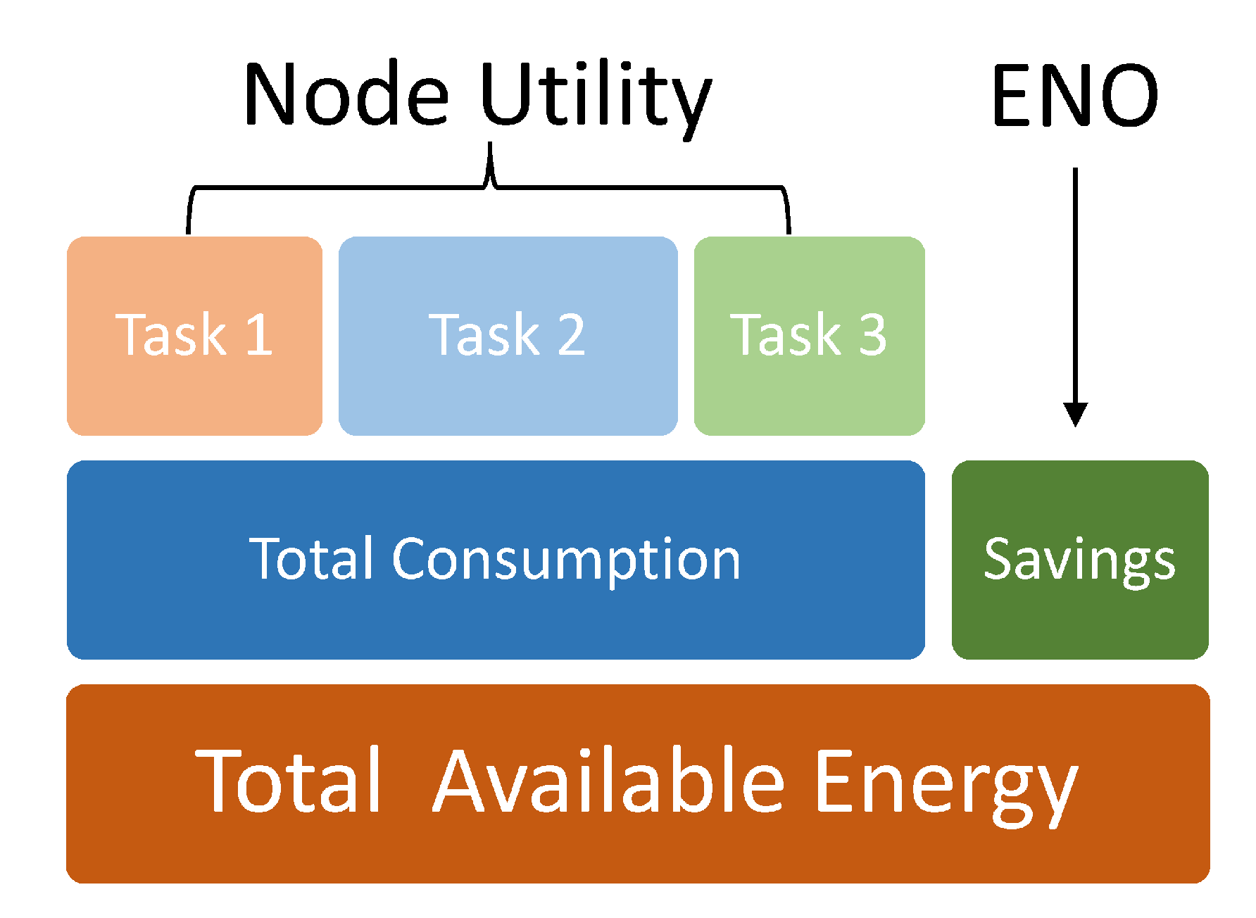
• ensure that the node does not violate energy neutrality in the long-term by regulating the gross node energy consumption
• proportion of the budgeted energy between different tasks.
• dynamically tradeoff between maximization of different objectives w.r.t. user-defined priorities.
• achieve all of this using much fewer computational requirements than existing methods.

We use a general EHWSN model described in [19], and:

• develop a suitable MDP for both SORL and MORL implementations. Furthermore, we perform comprehensive experiments to analyze how our proposed MDP overcomes the limitations of traditional definitions to achieve near-optimal solutions.
• analyze the effect that different reward incentives and environmental factors have on the learning process as well as the resultant policies.
• demonstrate that our proposed algorithms can overcome the limitation of traditional MORL methods for ENO and learn better policies at lower costs.

We organize this work as follows. In Section 2, we briefly discuss previous research in the area and its limitations. We describe the general EHWSN system model in Section 3 for which we develop our MORL framework. We give a brief theoretical background for ENO and RL in Section 4. In Section 5, we describe the MDP and our proposed algorithms that constitute the MORL framework. The experimental setup is explained in Section 6. We then simulate single-task and dual-task EHWSNs extensively using our proposed framework. We give a comprehensive analysis of our results in Section 7 our conclusions in Section 8.

2. Related Work

2.1. Analytical Methods for ENO

Historically, ENO of EHWSNs maximized a single objective using analytical methods. They focused on maximization of either the gross device energy consumption [18,20] or the communication performance [21,22] using linear programming [18], non-linear programming [23,24], search methods [25], control systems [20], dynamic programming [26,27] among other methods. While these approaches had comprehensive problem statements with formal proofs, they were very application-specific and required significant hand-tuning as well as non-causal information. We base our work on the mathematical foundation and the ENO goals in [18]. The authors provide a linear programming optimization approach that makes use of non-causal environmental data. They estimate the anticipated energy output and choose the duty cycle accordingly. They cater to battery inefficiencies and permit duty cycle adjustments to account for any variations in anticipated and actual harvesting circumstances. However, the efficacy of this method is highly dependent on the prediction mechanism and historical data. A non-causal solution proposed in [20] specified a battery-centric objective function. They restate ENO as a control system problem that minimizes the deviations in the battery level and achieves energy neutrality by using a linear quadratic tracker. The control system is reactive and somewhat adaptive to solar energy fluctuations. However, its stability requires careful calibration of hyperparameters depending upon the working environment. Similar control system solutions are also presented in [28,29]. Our RL-based solution relies very little on the prediction mechanism and any hyperparameter tuning required is a one-time effort. It therefore can be applied across many different application domains with little to no change.

In [29], the authors extend the problem statement by incorporating the time-varying utility of the data gathered by the sensor node. They argue that the sensing rate should vary depending on the utility of the sensed data as perceived by the user. They take the example of a soil moisture sensor system that exploits the prior knowledge of the seasonal cycles of rainfall. In this scenario, the utility of sensed data is low when there is no rainfall. Therefore, the authors propose a heuristic solution that conserves energy by reducing the duty cycle when there is little rainfall (low data utility) and increasing the duty cycle when there is rain (high data utility). Although data-utility is an important parameter to consider during energy scheduling, we do not always know how the data utility varies. This work assumes prior knowledge of this variation. Our proposed solution on the other hand does not require any prior information and optimizes the energy policy even if the data utility may vary unexpectedly.

2.2. Single Objective RL Methods for ENO

Analytical methods are unscalable and non-adaptive solutions that require significant design bias. RL methods emerged as an alternative on account of its common algorithmic paradigm to learn adaptive policies that could be applied to a wide variety of applications (i.e., scalable solutions). Early applications of RL in EHWSNs concentrated on optimizing simple communication policies [30,31,32,33,34,35] under the assumption that communication tasks consume the majority of the energy. These methods were superior to analytical methods but required complicated hand-crafted definitions of the states, actions, and reward functions. Since EHWSNs interact with the real world (i.e., an open system), it is very difficult to define the states and actions for an RL MDP that can sufficiently capture the environment dynamics without making the RL problem too complex to solve. More importantly, the ENO reward feedback is very long-term and delayed and so it is difficult to define a reward function for convergent, stable, and robust RL solutions. Non-optimal definitions result in increased learning costs for the nodes which translate to increased learning time, computation requirements, and “catastrophic mistakes” (unsafe exploration actions) made during learning.

Solutions presented in [26,36] use specialized reward functions that are difficult to design. They may also sometimes lead to unexpected behavior due to reward hacking [37,38,39]. In our previous paper [9], we devised a simpler, general reward function capable of learning adaptive policies using tabular RL. The paper also demonstrated the adaptivity of RL algorithms to changes in climate, device parameters, and battery degradation. Other similar research related to RL for ENO include [40,41,42].

2.3. Multi-Objective Optimization Methods

Most research related to ENO of EHWSNs (both analytical and RL-based) approaches usually assume maximization of some single proxy objective such as duty cycle/sampling rate [7,8,9,40,42,43,44] or communication-based metric such as maximizing throughput/bitrate and minimizing packet loss/latency [5,6,45,46,47,48,49]. However, realistic implementations usually require optimizing over multiple objectives. There has not been enough research on energy scheduling among multiple tasks w.r.t. different objectives in EHWSNs. This is very important, especially for modern resource-constrained sensor nodes.

It is still not very clear what is the best way to learn policies using multiple sources of reward signals. One common approach is to employ scalarization techniques to transform the multi-objective problem statement into a single-objective one, and then apply conventional RL algorithms to solve it. Scalarization consolidates the multiple rewards by some function to a single value [7,50,51,52].

One scalarization technique is to multiply the rewards together and scale the product as in [7,50,52]. In such a case, it is not very clear what objective is being emphasized. These methods do not allow for the optimization of any one specific preference; instead, they learn an “average” policy across the space of preferences. Another scalarization approach is to multiply the rewards by different weights and sum them together [51]. This allows the user to specify which rewards the policy should emphasize i.e., tradeoff between different maximization objectives. However, this requires the relative weights of the different rewards to be known before training. The learning process would have to be repeated separately for different weight configurations. Consequently, the user has to store a different policy for each unique preference which is unscalable and resource intensive. Ideally, we would like an RL method that can trade off between the maximization of different objectives during runtime (after the node has been trained and deployed). Thus reward scalarization methods have significant drawbacks that hinder their use for MORL in EHWSNs. This is explored in more detail in [3,52].

Another method to learn from multiple reward signals would be to integrate them into the RL MDP as a reward vector. Such MORL methods are generally available as single-policy methods and multi-policy methods. Interested readers can find a good overview of general MORL methods in [53]. With single policy techniques, the agent learns policies for multiple conflicting objectives whose preferences are not known a priori. However, it is difficult for a single model to learn the best policies for various preference scenarios. These methods generally involve learning an action-value function that takes into account the relative emphasis among the objectives [14,54,55]. For e.g., in [14], the authors modify the Bellman equation to learn a single parametric representation for optimal policies over the space of all possible preferences. They evaluate their method for video game domain problems. A limitation of this work is that the proposed MDP and the corresponding multi-objective Bellman equation are applicable only for discrete action spaces where performing an argmax search over the Q-values is feasible. This does not hold for continuous action spaces. We would like a general MORL method that accommodates both continuous states and action spaces. Multi-policy methods learn a set of policies in order to approximate the Pareto-frontier [12,13,56,57,58]. The computed policies encompass the entire space of possible preferences. These methods require considerable computation resources and have scalability issues because the learned policies can grow significantly with the domain size. For example, in [58], the authors propose to decompose a MOO problem into several simpler single-objective problems and solve for each Pareto solution using DRL. They then propose to generate the Pareto-frontier by combining the different Pareto solutions. Since this is a computationally expensive process, they propose to reuse weights of neighboring sub-solutions to accelerate the convergence of each of the Pareto solutions. Furthermore, they argue that DRL has good generalization properties and can be extended to more complex optimization with no training. This work has a similar approach to MOO as our method in that it interpolates between different Pareto solutions to find a locally optimal one. However, the method in [58] is quite difficult to implement in IoT embedded devices because it employs computationally intensive techniques such as attention mechanism and recurrent NN in addition to the actor-critic model. Furthermore, due to the time-varying objective functions in embedded systems, it would be very difficult to compute the solutions from all the sub-models at every timestep. Our method sidesteps this issue by computing only the greediest Pareto solutions and interpolating between them. While this sacrifices some optimality, our method is less compute-intensive.

Contemporary MORL methods are insufficient to solve the ENO problem for MDPs due to a limited MDP and high computation requirements. We, therefore, use our MORL framework to solve the energy scheduling issue for EHWSNs in this work. Our system uses a standard Deep Deterministic Policy Gradient (DDPG) algorithm [59]. DDPG has been used for single reward maximization in [46,47] for communication tasks. Here, we use DDPG for MORL primarily because it can accommodate continuous states and actions while being comparatively less computationally intensive. More powerful RL algorithms are also available, but they require significantly more computational resources.

In [60], the authors also use DDPG to learn multiple tasks from reward vectors. Similar to our approach, they also use a reward vector to learn multiple value functions simultaneously. This is in contrast to standard single-objective RL methods that use a scalar reward signal to learn a single value function. However, this work focuses on multi-task learning. It assumes the tasks are exclusive (i.e., do not occur simultaneously) and independent (i.e., the objectives are non-conflicting and therefore no tradeoffs are necessary). In short, this work is not a multi-objective optimization problem where tradeoffs need to be made.

Our work is also closely related to [61]. They also use MORL DDPG for an autonomous driving application scenario. In this work, different agents learn policies for different tasks and collectively form a combined policy. However, their method uses a Thresholded Lexicographic Ordering (TLO) method. This requires the user to specify the preferred ordering over objectives and their thresholds prior to training. As explained previously, this is generally not possible because the users usually adjust their preference after the node has been deployed. The alternative of storing policies for all possible orders and thresholds is not scalable.

Our proposed MORL MDP and algorithms can learn intelligent policies at lower costs by using continuous state and action spaces from multiple reward sources using a reward vector. Furthermore, our proposed algorithms can learn to tradeoff between multiple objectives at runtime, similar to single-policy MORL methods but using much less computational resources than single-policy and multi-policy methods.

Since we concentrate on MOO with MORL in this work, we have yet to address issues of intermittent computing, task dependency, and network-based optimizations in IoT systems. An alternative approach for consolidating multiple objectives may be a game-theoretic/multi-agent approach as explored in [62,63].

Although we have focused our discussion on MOO for energy scheduling in EHWSNs until now, MOO solutions are quite popular in IoT systems when they focus on holistic network performance rather than individual node energy-neutrality. These works primarily target issues like sensor node deployment configuration to maximize coverage and lifetime [64,65,66] or optimizing the routing parameters while reducing the latency and energy consumption [67,68]. It is possible to solve these problems with traditional heuristics because they are defined with time-invariant objective functions [69,70]. As to our knowledge, MOO in IoT systems for optimization problems with time-variant objective functions (e.g., duty cycling optimization for EHWSNs) has not been discussed enough. Hence, we propose our low compute MORL framework to optimize problems with time-varying objective functions.

3. System Model

Figure 2 assumes a harvest-store-use solar EHWSN that is required to be always on. Although this system model is specific to multi-task EHWSNs for optimizing energy usage, it can be easily adapted for other resource-scheduling problems in IoT embedded systems. The EHWSN is equipped with an energy harvester and a finite energy buffer. We assume a battery for the sake of example but any other type of energy buffer can also be used (e.g., super-capacitors). The user requests the node to execute various tasks relating to sensing, communication, and processing. Each task request has an associated energy demand to satisfy various performance requirements (e.g., sensing rates [29] and transmission throughputs [6,7]).

The MORL agent optimizes energy usage in discrete timesteps. It intelligently distributes the energy across various tasks at each timestep. Each task generates a task-utility depending on how much energy it was allocated. The weighted sum of all task-utilities gives the node-utility. The agent’s objective is to maximize node utility.

The energy required to fully conform to the user’s request to execute the ith task is $d_t^i\in [z_{min}^i,z_{max}^i]$. $d_t^i$ is determined by the user/application and generally varies with time [7,29]. For example, a sensing task request may have a high energy demand d corresponding to an increased sensing duty cycle; or the user may request a higher QoS thus increasing the energy demand for a transmission task.

The MORL agent observes its environment (the system state) at timestep t to decide the task energy, $z_t^i\in [z_{min}^i,z_{max}^i]$. It can under-provision a task to conserve energy by sacrificing task performance. The amount of under-provisioning is represented by the conformity factor $k_t^i\in [0,1]$. The actual energy allocated to task i is $z_t^i=max(z_{min}^i,d_t^i\times k_t^i)$. $z_{min}^i$ represents the minimum energy required to run the task. (If $z_t^i<z_{min}^i$, the task fails.) The task-utility is given by $u_t^i=min(1,U^i(z_t^i/d_t^i))$, where $U^i$ is a monotonically non-decreasing function. Since over-provisioning energy to a task does not result in increased utility, we constrain the task-utility to be $u_t^i\le 1$.

Our proposed system model improves over traditional system models by explicitly allowing the agent to under-provision the task energy and also preventing any over-provisioning. Traditional solutions usually did not consider the time-varying utilities of tasks and opportunistically maximized duty cycles [8,9]. For e.g., if the objective were to maximize the sensing rate, the node would reactively increase the sensing rate whenever energy is available [9,18,20] without taking into account whether the sensed data was useful to the user or not. However, as pointed out in [7,29], task utilities generally vary with time and it would be wiser to expend energy in periods of high utility over low utility. With our system model, it is possible for the MORL agent to under-provision tasks that have lower priority/utility for energy savings.

Energy Neutral Operation

For a node with n tasks, at time t, the battery level is $b_t\in [0,b_{max}]$, the harvested energy is $h_t\in [0,h_{max}]$, the total energy demand is $d_t={\sum }_{i=1}^n{d}_t^i$ and the energy consumed by the node is $z_t={\sum }_{i=1}^n{z}_t^i$ s.t. $z_{min}\le z_t\le z_{max}$. The charging/discharging losses of the battery are characterized by a function $\mathcal{B}\left(\right)$. The energy dynamics of the system are therefore given by $b_{t+1}=min(b_t+\mathcal{B}(h_t-z_t),b_{max})$.

Perfect energy-neutrality is guaranteed if $h_t-z_t=0\forall t$ although this might not always be possible or even desirable. For instance, the node must generally maintain a minimum level of operation at all times i.e., $z_{min}>0$ to account for the energy spent during sleep/listening mode or by the base sensing rate [10]; or the node may need to operate during the night ($h_t<z_t$). In other situations, it might not be best to greedily consume all the energy that has been harvested because some of it might be stored and used to extract more utility in the future. However, the node is energy-neutral if $\mathbb{E}\left[z\right]=\mathbb{E}\left[h\right]$ where $\mathbb{E}[·]$ is the expectation operator. This implicitly assumes that the EHWSN is designed to meet the request demands such that $\mathbb{E}\left[d\right]=\mathbb{E}\left[h\right]$. Causality constraints require that the cumulative node energy cannot exceed the cumulative harvested energy i.e., ${\sum }_0^t{z}_t\le {\sum }_0^t{h}_t$. The node is operational at time t if $b_t+h_t\ge z_{min}$. Otherwise, there is a downtime. When this occurs, the node becomes non-operational and consumes all of the energy harvested to recharge its battery to a user-specified level before starting up again.

One trivial policy may be to greedily maximize conformity at all times, i.e., $k_t^i=1$. This increases the risks of downtimes due to severe power depletion. Another trivial solution is to always operate the node at the minimum level of operation i.e., $z_t^i=z_{min}^i$. This leads to wastage of the potential utility of the node. The ideal energy management strategy would reduce downtimes while ensuring that all energy harvested is used wisely to maximize utility. The energy-neutrality of the node at time t is given by the Energy Neutral Performance (ENP) metric $e_t={\sum }_0^t\mathcal{B}(h_t-z_t)=b_0-b_t$, expressed as the total difference between harvested and consumed energy [7,8,9].

The ENP-utility is $u_t^{ENP}$, given by a function $U^{ENP}\left(e_t\right)$ which reflects the energy-neutrality of the node. The node-utility is a weighted sum of the individual task-utilities w.r.t. their priorities. For an EHWSN with n-tasks, the relative priorities between its $n+1$ objectives is expressed by ${\omega }_t=({\omega }_t^1,{\omega }_t^2,\dots ,{\omega }_t^{n+1})$ where ${\omega }_t^i\in [0,1]$ is the priority/preference for the ith objective. ${\omega }_t^{n+1}=(1-{\sum }_{i=1}^n{\omega }_t^i)$ is the implied priority for the energy-neutrality of the node. With a slight abuse of notation, for single-task EHWSNs, the priorities of task maximization and ENO are represented by ${\omega }_t$ and $(1-{\omega }_t$). The agent’s ultimate objective is to maximize the overall node-utility $w_t={\sum }_{i=1}^{n+1}{u}_t^i{\omega }_t^i$. If the node had infinite energy, the obvious policy would be to maximize $u_t^i$ for all tasks. However, due to severe energy constraints, the MORL agent has to decide which utilities to maximize and by how much w.r.t. the user’s priority.

It is important to note that $u_t^i$ and $w_t$ denote the instantaneous utilities. They do not reflect long-term returns and therefore cannot directly quantify the effectiveness of the policy. For instance, in the case of a solar EHWSN, the instantaneous ENP $e_t$ does not give us much information about the long-term energy-neutrality of the policy because it is expected to fluctuate over the course of a day. Thus, to compare and improve policies, we require the notion of the value of a policy which we discuss in the following section.

4. Theoretical Background

In this section, we introduce the Deep Deterministic Policy Gradient (DDPG) RL algorithm [59] and describe the MOMDP for MOO using RL.

4.1. Single-Objective RL

In a standard SORL, an agent observes the state of its environment $s_t\in \mathcal{S}$ at each timestep and then performs an action, $a_t\in \mathcal{A}$, in accordance with some policy $\pi \left(a\right|s)$. As a result, it moves on to the next state $s^{\prime }$ and receives a scalar reward $r_t$ reflecting how optimal the action was in relation to the optimization objective. The rewards are presented via the reward function $\mathcal{R}(s,a,s^{\prime })$ and are typically discounted by $\gamma \in [0,1]$. The procedure then restarts once the agent achieves a terminal state (the conclusion of an episode). The agent learns progressively better policies that maximize its cumulative reward using the rewards and its prior experiences. An episodic discounted Markov Decision Process (MDP) is used to model this sequential decision-making situation. The MDP is defined by a tuple $(\mathcal{S},\mathcal{A},\mathbb{P},\mathcal{R},\gamma )$ where $\mathcal{S}$ is the continuous state space, $\mathcal{A}$ is the continuous action space and $\mathbb{P}\left(s^{\prime }\right|s,a)$ defines the transition probability from state s to $s^{\prime }$ as a result of action a.

The Q-value of a state-action pair $Q^{\pi }(s,a)$, w.r.t. policy $\pi$, gives the expected return when executing action a from state s as defined in Equation (1a) for an episode of length T. It can be computed recursively by using the Bellman equation in Equation (1b).

$$Q^{\pi }(s,a)={\mathbb{E}}_{\pi }\left[\sum _{t=0}^T{\gamma }^{t}R(s_t,a_t,s_{t+1})|s_0=s,a_0=a\right]$$

(1a)

$$Q^{\pi }(s,a)={\mathbb{E}}_{\pi }[R(s,a,s^{\prime })+\gamma Q(s^{\prime },\pi \left(s^{\prime }\right))]$$

(1b)

The main idea behind RL is for the agent to learn a policy to select an action that maximizes the Q-value for each state that it encounters (procedural knowledge). This requires learning the Q-values of all state-action pairs (predictive knowledge). We approximate the Q-values with a neural function approximator $Q_{\theta }(s,a)$ parameterized by $\theta$ (the critic). The policy is output by a function ${\pi }_{\varphi }\left(s\right)$ with parameters $\varphi$ (the actor).

We employ the Deep Deterministic Policy Gradient (DDPG) [59] RL algorithm for this work. DDPG is an off-policy actor-critic formulation. Off-policy points to the fact that the algorithm can learn the Q-function for a policy $\pi$ although its training examples may be obtained from a (slightly) different policy. This off-policy behavior will be crucial later on when we have to learn policies with different objectives from the same set of training examples.

Previous RL solutions were limited because they used discrete state-action spaces [7,9]. We opt for DDPG because it supports continuous states and actions. It is also simpler to implement in comparison to other RL algorithms of similar nature for continuous control. The DDPG critic evaluates the Q-value of state-action pairs whereas the actor outputs a deterministic action for a given state. To encourage exploration, some random noise is added to the actor’s output during the learning phase. We also maintain time-delayed versions of the actor and critic referred to as target networks [15], $Q_{{\theta }^{-}}(s,a)$ and ${\pi }_{{\varphi }^{-}}\left(s\right)$, to increase learning efficiency and stability. The parameters of the target networks are updated by Polyak averaging with the parameters of their main counterparts.

During training, the agent collects experience tuples $(s,a,r,s^{\prime })$ at each timestep t and stores it in an experience replay buffer [15]. At each training step, a random minibatch $\mathbb{B}$ of experiences are selected and a gradient descent is performed to minimize the loss functions in Equations (2a) and (2b).

$$L(\theta ,\mathbb{B})={\mathbb{E}}_{\mathbb{B}}\left[Q_{\theta }(s,a)-(r+\gamma Q_{{\theta }^{-}}(s^{\prime },{\pi }_{{\varphi }^{-}}\left(s^{\prime }\right))\right]$$

(2a)

$$L(\varphi ,\mathbb{B})=-{\mathbb{E}}_{\mathbb{B}}{Q}_{\theta }(s^{\prime },{\pi }_{\varphi }\left(s^{\prime }\right))$$

(2b)

Minimizing Equation (2a) gives more accurate estimates of expected return in taking a particular action in a particular state. On the other hand, minimizing Equation (2b) corresponds to choosing the action that maximizes return (or Q-value) from a given state.

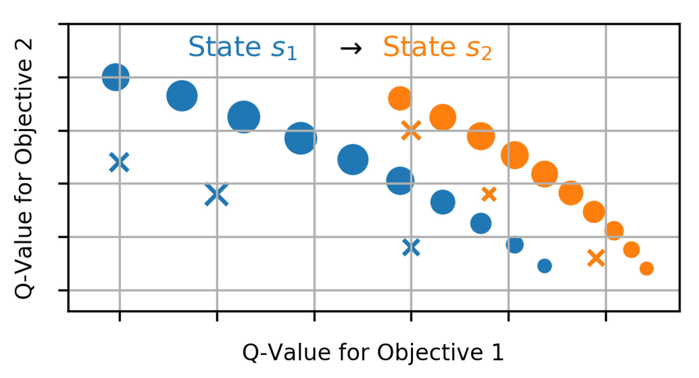
4.2. Multi-Objective RL

In a typical MOO problem, an optimizing variable is mapped into a multi-dimensional objective space by objective functions. Pareto-optimal points are those mappings in which one objective’s value cannot be increased without lowering the value of at least one other objective. The utility corresponding to the value of the optimizing variable is given by the linear combination of its mapped objective values weighted by user-defined priorities (We do not cover non-linear utility functions in this work).

Most popular MOO solutions assume a time-invariant objective function. In such a case, Evolutionary Algorithms (EA) or Monte Carlo (MC) rollouts are used to map a sample population of the optimizing variable to points in the objective space. This usually takes many rollouts/generations. By doing so, we hope to either find the value of the variable that has the highest utility or approximate the Pareto-frontier with some function or visualization technique. These methods have been used extensively in the optimal positioning of sensor networks which involves a tradeoff between the conflicting objectives of node lifetime, coverage, and cost within the computation, energy, and communication constraints [67]. For e.g., in [71], the authors use GA to minimize energy consumption and node count while maximizing coverage for a sensor network. They assume that the nodes are statically deployed and that the Quality of Service (QoS) remains constant. Each optimization process takes hundreds of generations to converge. This approach works for this particular problem because the working environment (optimization space) does not vary drastically from one generation to another i.e., the optimization problem is time-invariant.

Unfortunately, these methods are not very useful when the objective function is time-variant like in the case of energy optimization of EHWSNs with variable energy availability at each time step. In our case, the RL agent has to output an action at every timestep such that it trades off between the different objectives. The agent’s action $\pi \left(s\right)=a$ is the optimizing variable in this case. The objective functions are the Q-functions $Q^{\pi }(s,a)$ because they quantify how the actions will ultimately affect the long-term cumulative payoff. $Q^{\pi }(s,a)=Q^{\pi }(s,\pi \left(s\right))$, however, is parameterized by the state s, which evolves at every timestep. Figure 3 illustrates this, showing how the same set of sampled actions map to different locations in the objective space as the state changes from $s_1$ (blue) to $s_2$ (orange). Thus, due to the time-varying nature of the objective space, using elitist multi-objective optimization techniques like Monte Carlo (MC) rollouts or Evolutionary Algorithms (EA) is particularly unfeasible. If one were to use, say MC, one would have to sample many rollouts, approximate the Pareto frontier, and find the solution with the best utility at every time step. This requires very fast and very powerful computation which is not possible in sensor nodes or similar embedded systems.

Thus, we propose a MORL framework in Section 5. Our framework learns the Q-functions and policies that can deduce the best action to maximize utility from Pareto-frontier. We first develop a general Multi-Objective Markov Decision Process (MOMDP) for MORL with m objectives. $\mathcal{S}$ is the continuous state space, and $\mathcal{A}$ is the continuous action space. The reward function is now a vector function, $\overrightarrow{R}(s,a)=[R_1(s,a),R_2(s,a),\dots ,R_m(s,a)]$ and the discount factors corresponding to different objectives are given by $\gamma =[{\gamma }_1,{\gamma }_2,\dots ,{\gamma }_m]$. The transition probability from s to $s^{\prime }$ due to action a is given by $\mathbb{P}\left(s^{\prime }\right|s,a)$. The Q-function is also a vector function $\overrightarrow{Q^{\mu }}=[Q_1,Q_2,\dots ,Q_m]$ whose elements represent the different objective functions. $\mu$ is the MORL policy that extracts the Pareto-optimal action w.r.t. the user-preference $\omega \in \mathsf{\Omega }$. The next section describes how we create a suitable MOMDP for EHWSNs and how the agents can learn the vector Q-functions to extract the optimal actions. $\mathsf{\Omega }$ determines the space of preferences among the m objectives. The MORL policy $\mu$ is now associated with an m-dimensional vector Q-value function $\overrightarrow{Q^{\mu }}=[Q_1,Q_2,\dots ,Q_m]$ whose components correspond to the different objective functions. $\mu$ extracts the Pareto-optimal action w.r.t. the user-preference $\omega \in \mathsf{\Omega }$. In the following section, we develop a suitable MOMDP for EHWSNs and present solutions to learn the vector Q-functions and extract the optimal actions.

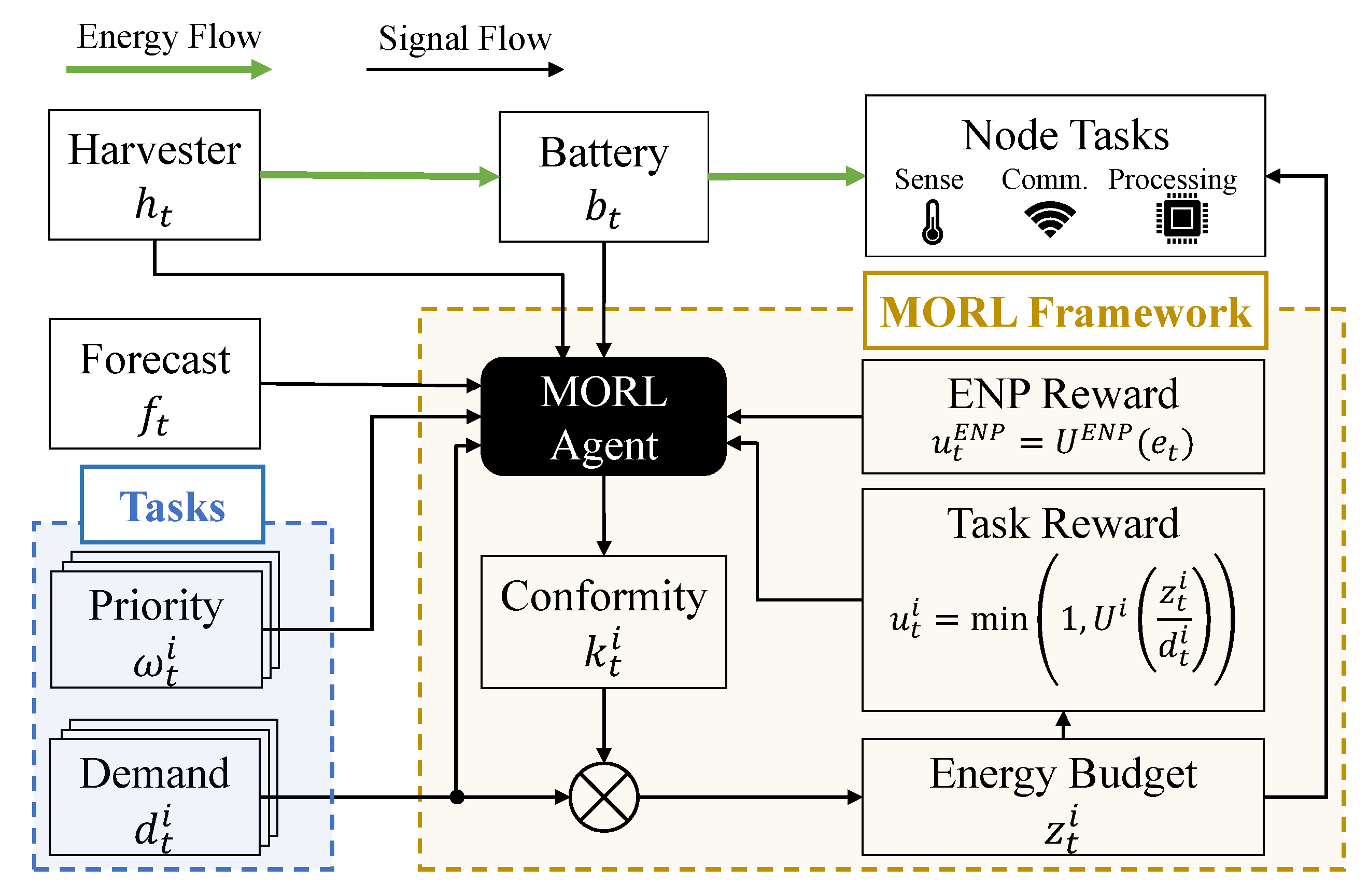
5. Proposed MORL Framework

5.1. MOMDP Formulation

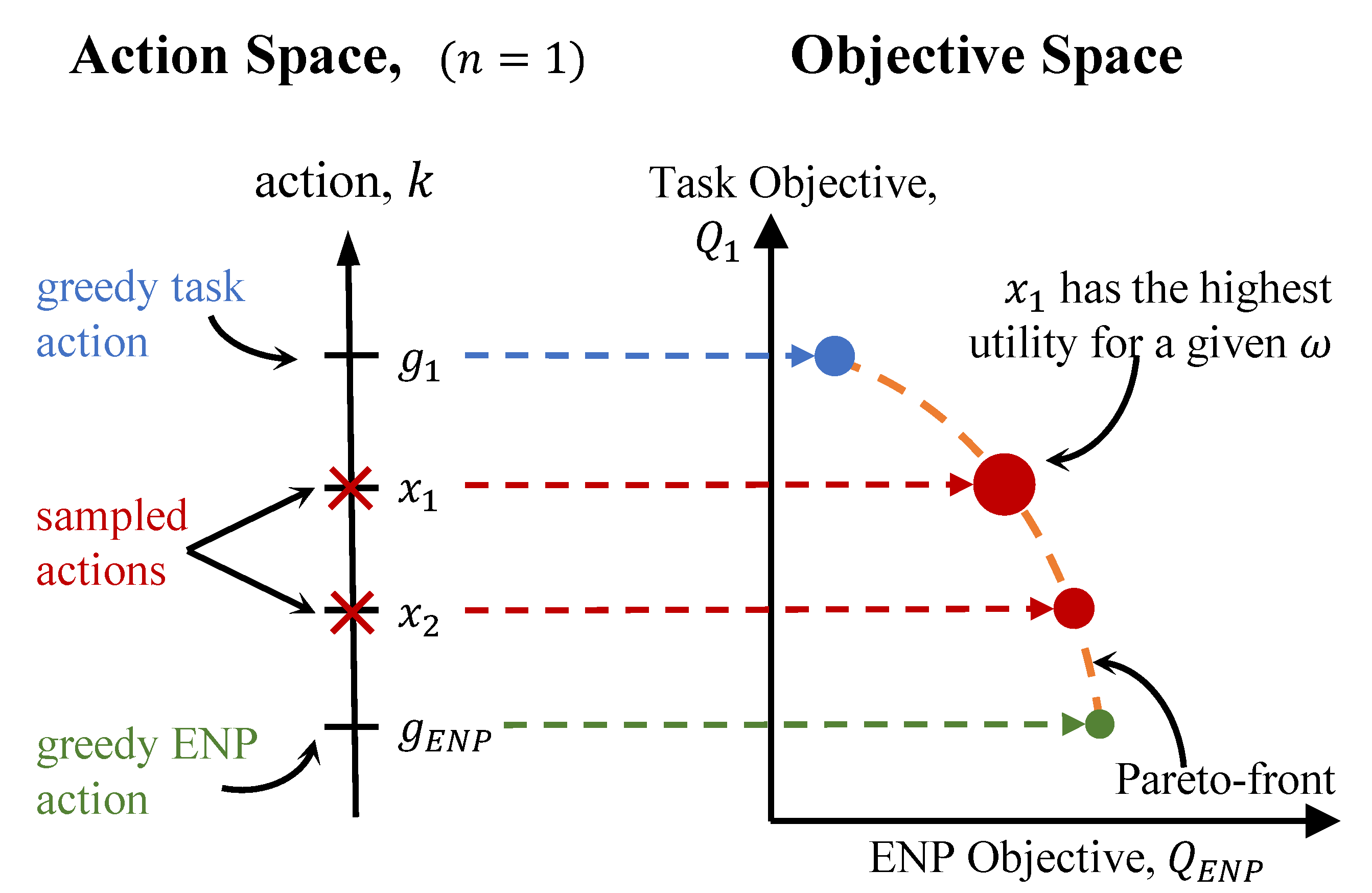
Here we define the reward function and the state-action space of our MOMDP for the system model in Section 3. Although the following description is specific to the energy-scheduling problem in EHWSNs, the general idea behind the MOMDP formulation is applicable for any type of resource-scheduling problem in IoT embedded systems.

Multiple Reward Functions: Since modern EHWSNs have multiple objectives, a reward function that supports multiple sources of rewards is needed. In previous methods where multiple objectives are projected into a scalar by scalarization, the rewards become noisy and obfuscate the actual objectives. The biggest downside is that tradeoffs cannot be made at runtime [51] because the relative weights between objectives need to be known and fixed before training. Another drawback is that scalarization sometimes involves intricate reward shaping which introduces considerable design bias [7,52,72]. Our framework learns from distinct, independent reward signals to get around these restrictions without any complex reward shaping. Each of these reward signals represents a single optimization target. In our framework, the task rewards are the task utilities, and the ENO reward is the ENP-utility.

Well-defined state space: Our framework defines the state at time t by a tuple $s_t=(\tau ,b_t,\overline{b_t},h_t,f_t,d_t)$. $d_t=(d_t^1,d_t^2,\dots ,d_t^n)$ is a tuple containing the different task requests and $h_t$ is the harvested energy. Our state definition includes important temporal information (which are not present in previous works)—(i) $\tau$ which represents the time of the day, (ii) $\overline{b_t}={\sum }_{k=0}^T{b}_{t-k}/T$ which is a moving average of battery values over a horizon T, and (iii) $f_t\in [0,1]$ which is a rough prediction of future energy supply as in [9]. By making these additions to the state definition, the learning process is stable and faster compared to earlier research [7,50].

Safe Actions: RL learns through exploration and mistakes are inevitably necessary during the initial stages of training. These mistakes need to be minimized in the real world because they lead to loss of utility and may have potentially unintended consequences, e.g., node shutdown due to energy depletion. Previous RL formulations define actions so that they directly correspond to the energy consumption of the node, e.g., the node duty cycle or the transmission power [7,9,10,44,50]. This is dangerous because the agent may sometimes sporadically take very unreasonable actions (e.g., duty cycles suddenly spike causing battery exhaustion). This is usually due to maximization bias in Q-learning when using a discrete action space or defective policies owing to factors such as bad experience samples and learning instability.

In our formulation, we define the action to be the node’s conformity to various task demands. For an n-task EHWSN, the action is $k_t=(k_t^1,k_t^2,\dots ,k_t^n)$ where $k_t^i$ is the conformity of the node to the request $d_t^i$. This definition states that actions are safe because they never over-provision energy and hence avoid unintended battery depletion. As a result, the definition of our actions reduces the effects of catastrophic policies even if learning results in a bad policy, in contrast to action definitions in earlier techniques [7,9,50].

5.2. Runtime MORL

We now describe our first algorithm, Runtime MORL (Algorithm 1). This algorithm takes SORL actor-critic pairs trained with different reward functions as input. Each of these actor-critic pairs is trained to maximize a different objective. The algorithm uses these actor-critic pairs and generates a policy that can tradeoff between different objectives at runtime without additional training.

The action space of n-task EHWSN has $\left|k\right|=n$ dimensions. However, the EHWSN has to optimize across $n+1$ objectives, with energy neutrality as the $n+1$th objective. Algorithm 1 outputs each element of the action space using n pre-trained greedy actor-critic networks $({\pi }_i,Q_i)$. The ith task’s greedy conformance $g_i$, is output by ${\pi }_i$. The total conformance of the node $g_{ENP}$, with respect to the total demand $d={\sum }_{i=1}^n{d}^i$, is output by another pre-trained greedy actor-critic $({\pi }_{ENP},Q_{ENP})$. All greedily energy-neutral actions can be represented by a plane $g_{ENP}={\sum }_{i=1}^n{k}_i$, in the action space. The convex hull that contains this plane and all of the greedy actions is then determined.

Minimizing Computation Costs

One solution to finding the optimal action $k^{*}$ would be to learn a function that maps the entire convex hull to the objective space and then maximizes the node-utility using methods like gradient descent. This makes the learning problem very complex with extremely high computation and learning costs. Another solution would be to maintain a set of policies for each preference ($\omega$) but this is not a sustainable approach because $\omega$ takes continuous values. In Algorithm 1, we sample the locally approximate Pareto-optimal from the convex hull to determine the optimal action $k^{*}$. Algorithm 1 samples j actions $x_1,x_2,\dots ,x_j$ according to the user-preference $\omega =({\omega }_1,{\omega }_2,\dots ,{\omega }_{ENP})$. The core idea behind this approach is that when we progress from one greedy action to another along the convex hull, we are actually moving along the Pareto-front in the objective space and trading off between different objectives. This is possible in our case because we have assumed task-utility functions are a monotonically non-decreasing function of conformity (or action). The linear combination of the critics’ outputs $Q_i$ and $Q_{ENP}$, weighted by the task preferences ${\omega }_i$ and ${\omega }_{ENP}$, gives us the composite Q-values for each of these sampled actions. The action with the highest values is the most locally optimal action. When using Algorithm 1 in this way to determine the optimal action, a change in $\omega$ at runtime merely necessitates inferring the critics and recalculating the action-values, which is a relatively inexpensive process compared to gradient descent. By sampling more actions, we can increase the optimality of the solution with a corresponding increase in computation costs. Overall, compared to doing gradient descent to determine the best action, this technique uses far less processing. With this sampling strategy, we can always identify an action that is at least as beneficial as the greedy ones without making any assumptions about the concavity of the Pareto-frontier. This is important because concave Pareto-frontiers are a challenging problem for several MORL algorithms.

The implementation of Algorithm 1 for a scenario with a single-task optimization is shown in Figure 4. While $g_{ENP}$ greedily preserves energy-neutrality by decreasing the conformity k, $g_1$ greedily maximizes the task-utility by boosting conformity. Here, $g_1$ and $g_{ENP}$ define a straight line which is the convex hull. Two points on the line denoted by the red crosses are sampled using Algorithm 1. The outputs of the critics ($Q_1$, $Q_{ENP}$) are used to map the Q-values corresponding to all actions (both greedy and sampled) onto the objective space. These Q-values are weighted by $\omega$ and the best action is determined. In Figure 4, action $x_1$ is the best action since it has the highest composite Q-value (indicated by the size of the circles).

Algorithm 1: Runtime MORL.

5.3. MORL with Off-Policy Corrections

Now, let us focus on the scenario where there are no pre-trained, greedy actors and critics available; and greedy actors/critics have to be trained tabula rasa. With our second algorithm, Off-policy MORL (Algorithm 2), the critics learn their Q-values from the experience samples gathered from the agent’s interaction with the environment, while the actors simultaneously learn the greedy policies. Using Algorithm 1, the agent chooses actions that fall between the greedy actions based on the preference $\omega$ parameter. Thus, when implementing Algorithm 2, the critics must learn the Q-values $Q_i$ for a greedy policy ${\pi }_i$ from transitions generated by a different policy, say $\mu$. This requires off-policy corrections i.e., a method to compensate for the difference in state transition probabilities (s to $s^{\prime }$) between ${\pi }_i$ and $\mu$. We achieve this by multiplying the expected Q-values of the next state by their ratio of their transition probabilities, ${\rho }_i(s,s^{\prime })=\frac{\mathbb{P}\left(s^{\prime }\right|s,{\pi }_i)}{\mathbb{P}\left(s^{\prime }\right|s,\mu )}$ in Equation (3) where we use the approximation ${\rho }_i(s,s^{\prime })\approx {\omega }_i$. This approximation makes sense (theoretical guarantees are not in the scope of this work) because $\mu$ is increasingly dominated by ${\pi }_i$ when ${\omega }_i$ is closer to unity and therefore does not significantly alter the expectation. However, when ${\omega }_i$ is extremely low, $\mu$ is considerably further away from ${\pi }_i$ and as a result, the expected return is proportionately decreased.

$$\begin{array}{cc}\hfill Q_i(s,a)& ={\mathbb{E}}_{{\pi }_i}[r^i+{\gamma }_i{Q}_i(s^{\prime },{\pi }_i\left(s^{\prime }\right))]\hfill \\ \hfill & ={\mathbb{E}}_{\mu }\left[r^i\right]+{\gamma }_i{\rho }_i(s,s^{\prime }){\mathbb{E}}_{\mu }\left[Q_i(s^{\prime },{\pi }_i\left(s^{\prime }\right))\right]\hfill \\ \hfill & \approx {\mathbb{E}}_{\mu }[r^i+{\gamma }_i{\omega }^i{Q}_i(s^{\prime },{\pi }_i\left(s^{\prime }\right))]\hfill \end{array}$$

(3)

Algorithm 2: Off-policy MORL.

6. Evaluation Setup

6.1. Simulation Environment

We test our framework by simulating solar EHWSN systems using data on solar radiation collected hourly by external rooftop pyranometers from 1995 to 2014 [73]. As a result, we chose an hour as the time interval for each timestep. We train the RL agents for the first ten years (1995–2004), and then measure their effectiveness over the following ten years (2005–2014). Each episode of our MDP lasts for one day (or 24 timesteps). The ten-year training period can be shortened to less than a year if we increase the granularity of the timesteps and adjust the discounting rates correspondingly. However, we maintain an hourly resolution for a fair comparison with previous methods [8,9]. An episode abruptly terminates with zero rewards when downtime occurs. In such a case, a new episode begins once the node has recovered. The parameters of the evaluated EHWSN system, normalized to $b_{max}$, are shown in

Table 1. Simulation Parameters.

Parameter	Maximum Value	Minimum Value
Battery, $b_t$	$b_{max}$	$b_{min}=10\%$ of $b_{max}$
Harvester, $h_t$	$h_{max}=5\%$ of $b_{max}$	$h_{min}=0$
EHWSN, $z_t$	$z_{max}=5\%$ of $b_{max}$	$z_{min}=0.5\%$ of $b_{max}$
Requests, $d_t$	$d_{max}=5\%$ of $b_{max}$	$d_{min}=0.5\%$ of $b_{max}$

. When $h_t=0$ (no harvested energy), the node can deplete 5% of the battery per timestep. This means that the node can drain a fully charged battery within 20 h at maximum power and takes 200 h (≈8 days) at minimum power with no energy harvesting. These parameters are based on a realistic EHWSN [74] with a current rating of 100 $\mathrm{m}$$\mathrm{A}$ equipped with a 2000 $\mathrm{m}$$\mathrm{A}$$\mathrm{h}$ battery. As soon as the battery capacity falls below 10%, the node enters recovery mode and is reset. To simplify comparison and analysis, we assume this recovery is instantaneous without loss of generality. The request function generates the task demands (or requests) at random so that $\mathbb{E}\left[h_t\right]\approx \mathbb{E}\left[d_t\right]$. This guarantees that ENO is indeed achievable. The rolling average of $h_t$ for the following 10 days is added with some random noise to provide a rough estimate of the weather forecast $f_t$.

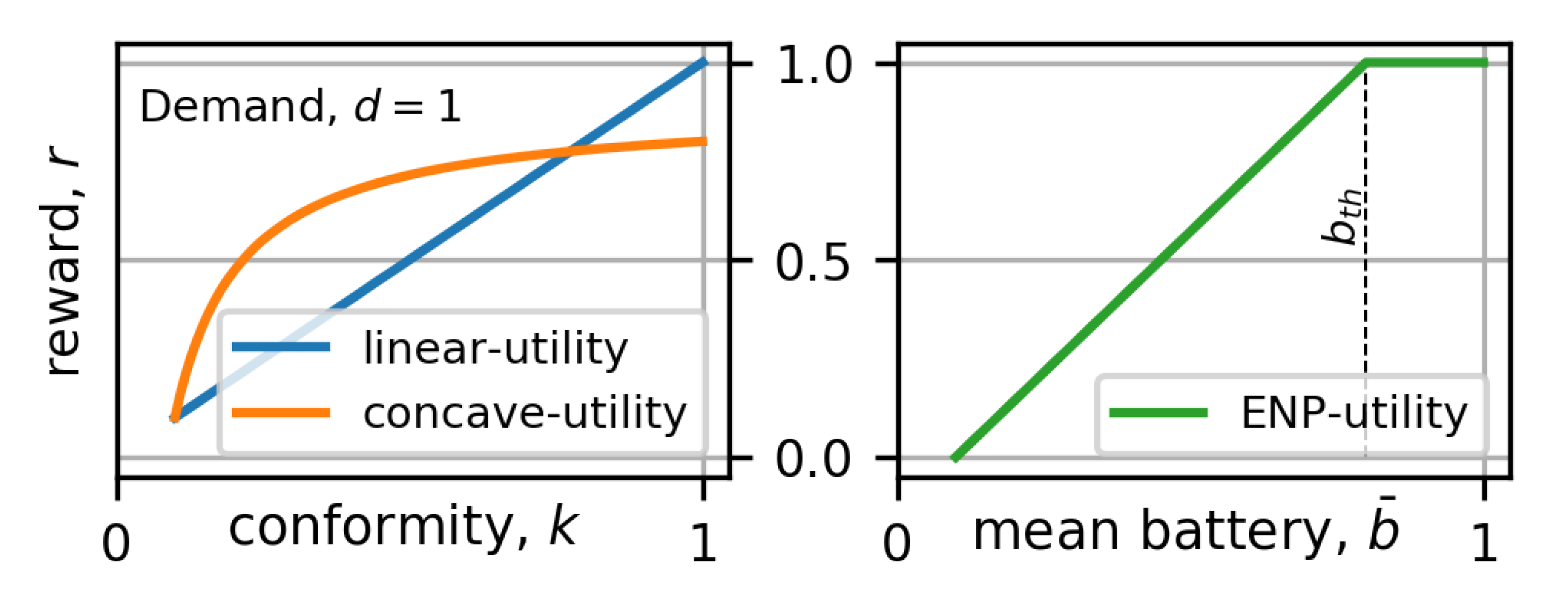
6.2. Utilities and Reward Functions

We use single-task (bi-objective) and dual-task (tri-objective) EHWSNs for our evaluations. The single-task node increases the node conformity linearly in compliance with the user demand while retaining long-term energy neutrality to maximize sense-utility [9,18,20,29]. Thus, we establish the rewards for maximizing the sensing rate by the sense-utility $u_t^{sense}$, which increases linearly with conformity (energy usage) in accordance with the linear-utility function in Figure 5 (left).

The ENP-utility $u_t^{ENP}$ corresponds to the rewards that represent the energy-neutrality of the node given by

$$u_t^{ENP}=\left\{\begin{array}{cc}1,\hfill & \mathrm{if}\overline{b_t}\ge b_{th}\hfill \\ \frac{\overline{b_t}-b_{min}}{b_{th}-b_{min}},\hfill & \mathrm{otherwise}\hfill \end{array}\right.$$

(4)

Figure 5 (right) illustrates this reward function. $b_{th}$ is a user-defined battery threshold, and $\overline{b_t}$ is the moving average battery level over ten days. This reward function is similar to those in [7,8,9,52], but require less reward shaping. In addition, our reward function uses $\overline{b_t}$ instead of $b_t$ since it correctly captures the long-term temporal nature of ENO. $b_{th}$ is fixed at 80% of $b_{max}$ although this can be changed as needed. The relative preference between optimizing sense-utility and ENP-utility is reflected in $\omega$ for single-task EHWSN. $\omega =0$ places an emphasis on energy-neutrality whereas $\omega =1$ maximizes sense-utility.

We evaluate EHWSN systems that need to sense and transmit data when discussing dual-task EHWSNs. These nodes must increase their throughput in addition to maintaining energy neutrality and increasing their sense-utility. We assume a simplified transmission model with Binary Phase Shift Keying (BPSK) modulation with additive white Gaussian noise and Rayleigh fading. This is only for the sake of an example and can be modified as required. We do not consider the effects of multi-hop transmission and routing issues here because it adds another layer of complexity that does not directly pertain to the issue of MOO. For the sake of simplicity, we have assumed that a receiver is always ready to receive the data.

The node’s transmission throughput P is given by Shannon’s capacity formula $P=log(1+k)$ where k is the SNR of the transmission signal. In our case, the conformity $k=z/d$ is the SNR. The transmission task demand d can be interpreted as the amount of transmission power required to overcome channel noise and maintain the QoS determined by the user and z is the actual transmission power which results in throughput P. $u_t^{tx}=P$ is both the task-utility and reward. Higher SNR is necessary for higher throughput, but throughput does not increase linearly with higher SNR (transmission power). The concave-utility reward function in Figure 5 serves as a representation of this relationship.

Since the utility is non-linear, it may be wiser to use transmission energy to drastically improve the throughput when the channel is very noisy (∼ high demand) than to use the same amount of energy to increase the throughput by only a small amount when there is less noise (∼low demand).

The dual-task node must constantly choose how much energy to devote to transmission and sensing operations in order to increase throughput (or tx-utility) $u_t^{tx}$ and sense-utility $u_t^{sense}$ while maintaining long-term ENO (maximizing $u_t^{ENP}$). The tuple $\omega =({\omega }_{sense},{\omega }_{tx},{\omega }_{ENP})$ s.t. ${\omega }_{ENP}=1-({\omega }_{sense}+{\omega }_{tx})$ indicates the relative preference between the objectives.

6.3. Metrics

We compare the task-utilities of various solutions based on their yearly average. The total number of times the node enters recovery mode (i.e., downtimes) is used to compare the energy-neutrality of various solutions. Using downtimes as a metric for ENO is a more accurate reflection of the actual energy-neutrality than the ENP-utility and facilitates fair comparison. An intelligent policy strikes an equilibrium between increasing task utilities and reducing downtimes. The learning cost for a particular policy is determined by the number of downtimes that occur during the training period, with fewer downtimes being preferable (the training duration is the same for all RL agents). The node should ideally learn an energy management strategy with as little downtime as is feasible.

We perform each experiment with ten random seeds and average over them for comparison. The interquartile range (IQR) is indicated by the shaded regions and error bars (not shown in some figures for clarity).

7. Experimental Results

In this section, we present our results and answer the following questions:

• Do RL agents trained using the MDP (state and action definitions) based on our proposed general MORL framework perform better than heuristic methods and traditional RL solutions when optimizing for a single objective? Specifically, do they extract higher utility at lower learning costs?
• How well does the proposed Algorithm 1 tradeoff between multiple objectives at runtime using greedy SORL agents? How does it compare to traditional scalarization methods that are optimized using non-causal information?
• Can the MORL agents trained with our proposed MOMDP learn policies to maximize the tradeoff between different objectives? What is the cost of training in such a scenario?

A summary of the different SORL and MORL agents we evaluate is given in

Table 2. Single-Objective ENO Agents.

	Sense Objective, $\mathit{\omega }=1$	ENP Objective, $\mathit{\omega }=0$
Ours (RL Agents)	sense	enp
Ours (Smaller NNs)	tiny_sense	tiny_enp
Heuristic Methods	max_enp	max_k
Partially Markov States [7,9,10,44,50]		pomdp_enp
Absolute Actions [7,9,10,44,50]	raw_sense	raw_enp

and

Table 3. Multi-Objective ENO Agents.

Method	Name	Rewards/Values
Ours (Algorithm 1)	morl_runtime (2-task)	$\omega Q^{{\pi }_{sense}}+(1-\omega )Q^{{\pi }_{enp}}$
Ours (Algorithm 2)	morl_offpolicy (2-task)	$\omega Q^{{\pi }_{sense}}+(1-\omega )Q^{{\pi }_{enp}}$
Ours (Algorithm 2)	morl_multi (3-task)	${\omega }_{sense}{Q}^{{\pi }_{sense}}+{\omega }_{tx}{Q}^{{\pi }_{tx}}+{\omega }_{ENP}{Q}^{{\pi }_{enp}}$
Scalar Product [7,50,52]	mul_scalar	$u^{sense}\times u^{ENP}$
Scalar Sum [51,52]	add_scalar	$\omega u^{sense}+(1-\omega )u^{ENP}$

.

7.1. Single-Objective RL Policies Using Proposed MDP

7.1.1. Comparison with Heuristic Methods

Figure 6 shows the sense-utility and the corresponding downtimes experienced by the sensor nodes for a test period from 2005 to 2014 (ten years) under different policies. sense (red) and enp (green) are SORL agent policies ($\gamma =0.997$) that maximize sense-utility and ENP-utility respectively. We compare them with two heuristic policies, max_enp and max_k.

max_k represents the upper limit of utility maximization It greedily maximizes the sense-utility using a trivial policy that always conforms maximally ($k_t=1$) to all task requests without any consideration for long-term energy neutrality. As a result, it is also the least energy neutral with the highest number of downtimes. max_enp has the fewest possible downtimes and is, therefore, the most energy-neutral policy. It achieves this by increasing the node conformity with the battery level w.r.t. a non-linear function (shown in Figure 7). Greedy search and non-causal data were necessary to empirically establish the parameters of this function. max_enp indicates the upper limit of ENO because no policy can extract more utility than it does without increasing the frequency of downtimes.

In Figure 6, we observe that the energy neutrality (downtimes) of enp and max_enp are similar (green and blue bars). This means that enp is near-optimal w.r.t. the ENO objective. Using our MDP, enp performs as good as max_enp without the need for any non-causal information or empirical hand-tuning. Thus, we use enp as the baseline for ENO when comparing it with other RL agents. An RL agent would outperform enp if it has lower downtimes than enp and extracts higher sense-utility.

We also observe that sense is more aggressive than enp in maximizing utility. sense scores higher sense-utility than enp at the cost of larger downtimes. This is expected because sense was trained using only the sense-utility reward function and does not receive any direct feedback from the ENP-utility reward function. In spite of this, sense does not disregard energy neutrality like the trivial max_k agent which incurs very high downtimes (orange bars). sense learns to avoid downtimes so that it does not lose any opportunity to collect more rewards in the long term. This behavior is attributed to the discounting factor $\gamma$, which indirectly accounts for the ENO objective. We cannot conclude sense is optimal despite the fact that it extracts higher utility within competitive bounds of energy neutrality. A better solution would increase sense-utility while keeping sense’s downtimes constant. Since it is difficult to establish clear upper bounds in this situation, we compare other agents’ sense-utility against sense as a starting point.

Figure 8 illustrates the difference between the policies of sense and enp in more detail with their corresponding battery traces. The time interval shown corresponds to autumn/winter in Tokyo. It is very difficult to avoid downtimes during this period because opportunities to recoup any energy losses are very rare as the winter solstice approaches (Day 356). In fact, it is very difficult to avoid downtimes unless the node has full battery reserves on Day 260 and operates at its minimum duty cycle as much as possible. Consequently, sense, which is more aggressive in maximizing the duty cycle, experiences a downtime on Day 303 while enp maintains a conservative policy and passes the winter with no downtimes. After the winter solstice, both agents start to refill their battery reserves.

7.1.2. Adaptive Nature of RL Policies

RL solutions are superior to heuristic methods because they can adapt to changes in the working environment. Adapting policies to battery inefficiencies has been demonstrated in our previous works [8,9] using a simple model where these inefficiencies were lumped as increased node consumption. In this work, we use a more sophisticated battery model ($\mathcal{B}\left(\right)$ described in Section 3) that addresses the discrepancies in the charging and discharging efficiencies of the battery and the role it plays during the optimization of energy scheduling.

To investigate the effect of imperfect batteries in our framework, we compare the performance of sense with bad_batt in Figure 9 and Figure 10. bad_batt agent (purple) was trained and tested similarly to sense except that its battery charging efficiency was set to 50%. Figure 9 shows the battery traces and duty cycles for sense, enp and bad_batt in the beginning of the year when the days are shorter and so the solar energy is limited. enp consistently operates at the minimum duty cycle to conserve energy and avoid downtimes. sense tries to maximize the duty cycles during the night depending on how much is harvested during the day. Since sense has a perfect battery and there are no losses in storing and retrieving energy, it can play safe and choose to delay the maximization opportunities. On the other hand, bad_batt maximizes duty cycles mostly during the day. This way the energy from the solar panel can be directly fed into the node and energy losses due to battery charging and discharging can be minimized. Thus we see that the same MDP can learn very different policies to optimize different objectives and adapt to different working environments. This strengthens the case for using RL methods instead of heuristics for self-adaptive autonomous IoT embedded systems.

We also note that bad_batt is almost as optimal as sense in spite of its inefficiency (Figure 10). In fact, bad_batt seems to have better overall performance than sense with higher utility and lower downtimes. However, bad_batt has fewer stable policies than sense as evidenced by higher variations in performance (wider IQRs) among the ten different seeds that were evaluated. Thus, the presence of an inefficient battery may cause RL to learn policies that are more aggressive in maximizing utilities at the expense of the stability.

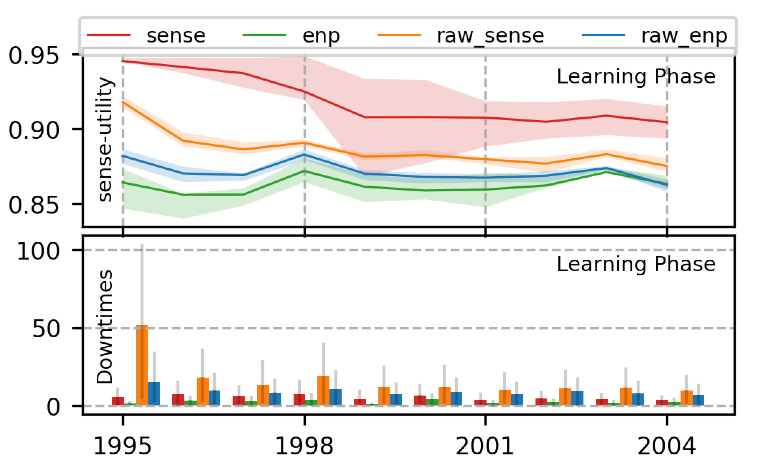
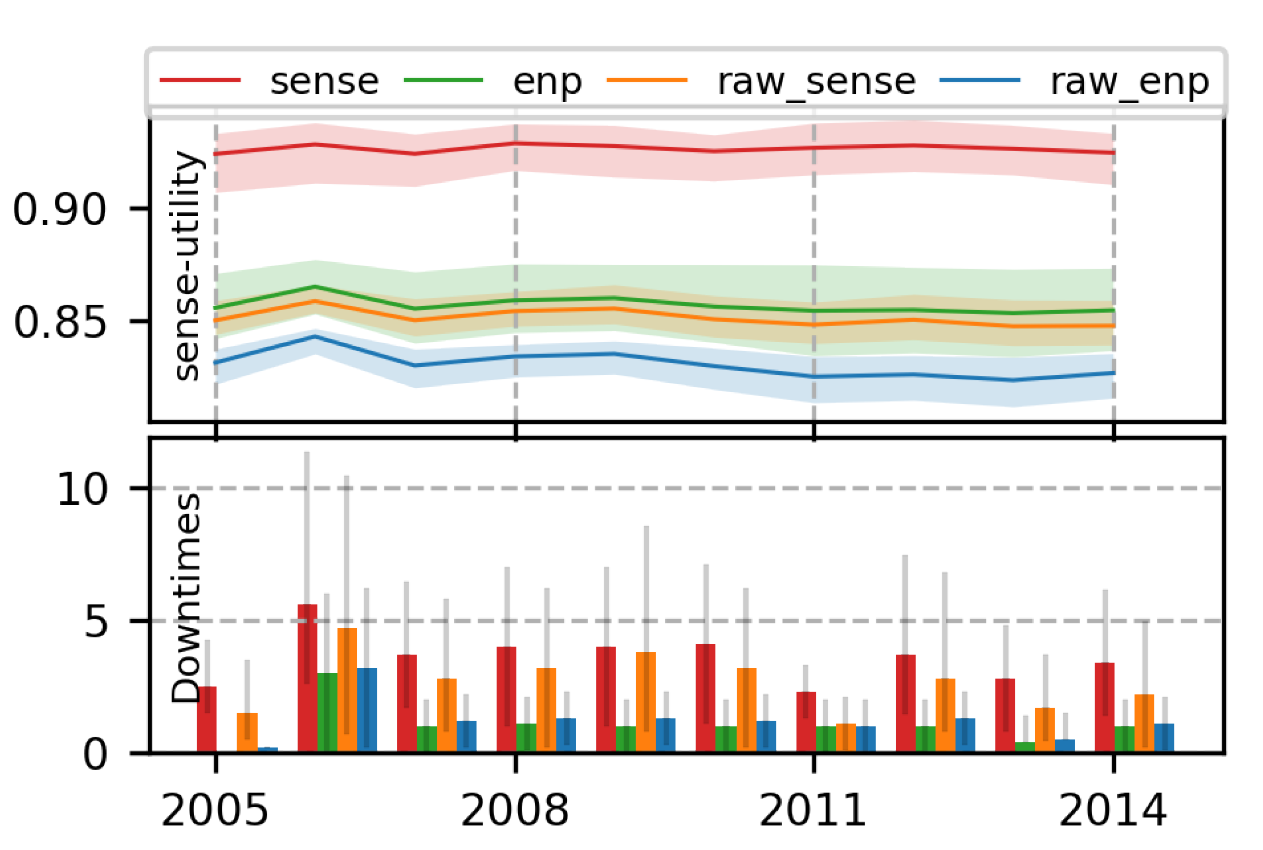
7.1.3. Superiority of Proposed MDP Formulation

Inclusion of temporal information for long-term optimization: The MDPs of previous methods [7,8,9,10,40,50] did not include sufficient temporal information in their state definitions i.e., the states were only partially observed. This resulted in unstable policies as well as larger learning costs. To study the effect of partially Markov states, we designate an agent as pomdp_enp that has omitted $\tau$ and $\overline{b}$ from its state definitions ($s_t=(h_t,f_t,b_t,d_t)$) and is trained to maximize ENP-utility using the same reward function and training environment as enp.

Since both enp and pomdp_enp are maximizing ENP, we are interested in how many downtimes they incur during learning and testing. Figure 11 compares the learning costs (top figure) and the test performance (bottom figure) between enp and pomdp_enp. We observe that enp (green) has lower learning costs than pomdp_enp (purple), which totals to approximately a 15% reduction. We also observe from the test results (bottom figure) that enp is also more energy neutral than pomdp_enp.

pomdp_enp is less optimal than enp because it does not have access to sufficient temporal information. This results in aliasing between different states. The result of such state aliasing is shown in Figure 12 which shows the battery and node energy traces for enp and pomdp_enp. At the beginning of Day 81, both agents are in the same state. However, pomdp_enp observes its state as only by the instantaneous values of $(h_t,f_t,b_t,d_t)$ whereas enp observes its state with additional temporal information: $\tau$ which represents the time of the day and $\overline{b_t}={\sum }_{k=0}^T{b}_{t-k}/T$ which is a moving average of its past battery values.

enp which has access to temporal information learns that it is okay to maximize duty cycles at dawn (because future energy harvesting possibilities will be available soon) but not at dusk (when there will be no chance of harvesting for a long period of time). We can observe this as the green spikes that occur at the beginning of the day (bottom figure). However, as far as pomdp_enp is concerned, the states before sunrise and the states after sunsets are the same because no energy is being harvested. So it (wrongly) learns to maximize the energy consumption both at dawn and dusk (purple spikes when there is no energy being harvested). This results in a very poor policy that has high learning costs.

Thus, we can see that sufficient temporal information is necessary to optimize for long-term ENO. Thus, our proposed MDP state definitions with sufficient temporal information enable learning more optimal policies at much lower costs. We also observe that the exclusion of temporal information does not affect the performance when maximizing sensing-utility (not shown). This is expected because optimizing policies with long foresight are not very important for sense-utility maximization.

Safer action definitions for efficient learning: In [29], the authors make the case that the utilities of the task vary with time and user requirements. They argue that it is more desirable to expend energy when the utility of the task is higher for the user than when the utility is low. Traditional RL methods did not take this time-varying utility of tasks into account and thus were not very energy efficient. One solution would be to include the user’s task demand $d_t$, into the state definition but our preliminary results show that this requires much more computation and is less stable when training. In our MDP, we propose to define actions as the conformity $k_t$ of the sensor node to the task demand $d_t$. This accommodates the time-varying nature of utility without an increasing problem complexity.

Another major advantage of our action definition is that it is much “safer”. Traditional methods defined the MDP actions as $z_t$, i.e., the amount of energy allocated to be consumed by the node at each timestep [7,8,9,10,40,50]. These action definitions led to high learning costs due to “catastrophic mistakes”. For e.g., during the exploration phase, there is nothing stopping an agent from driving the node at a very high duty cycle even when there is not enough energy available. This leads to node shutdown (downtime) which is very undesirable because we would like our nodes to be at least operational, albeit non-optimally, during the learning phase. After committing many such mistakes, the node learns to avoid downtimes but this raises the learning costs. With our action definition, even when the node explores using high conformity actions, the actual energy expended never exceeds the demand and is always relative to the demand. This forms a natural check against unnecessarily high energy usage and dangerous duty cycles thus minimizing downtimes and unsafe exploration.

We evaluate agents raw_sense and raw_enp and compare them with sense and enp to study the effects of action definitions during learning and testing. raw_sense and raw_enp are identical to sense and enp except that their actions are defined as the absolute allocated energy $z_t$. sense and enp define their actions as the conformity $k_t$.

In Figure 13 (bottom), we observe that our RL agents, sense (red) and enp (green), incur significantly less downtimes during learning compared to agents using traditional action definitions raw_sense(orange) and raw_enp(blue). This is especially true during the early training phase. For e.g., in the year 1995, the learning cost of raw_sense (orange bar) is extremely high even though it extracts much less sense-utility than sense (red). This is because the actions of sense are defined relative to the demand and therefore never over-provisions energy. This stops the node from exploring unnecessary and dangerous states. This is important during training because “bad” experiences can not only increase downtimes but also reduce the training stability. This is clearly observed in raw_sense (orange bar) also suffers from high IQR (which indicates unstable learning) as a result of inefficient learning. We observe that our action definition decreases downtimes by approximately 70% for both sense and enp w.r.t. raw_sense and raw_enp.

We also observe that the policies learned by raw_sense and raw_enp are inferior to sense and enp in Figure 14. When we compare enp and raw_enp, we observe that enp extracts much higher utilities than raw_enp although they have similar downtimes. This means raw_enp is losing out on many opportunities in maximizing utility. It is also very obvious that raw_sense is non-optimal. Although its downtimes are almost as high as that of sense, its utility maximization is much inferior to that of sense by a large margin. Thus, by defining MDP actions in a relative manner, the nodes can learn much better policies that incorporate the time-varying utility of tasks and reduce the learning costs dramatically.

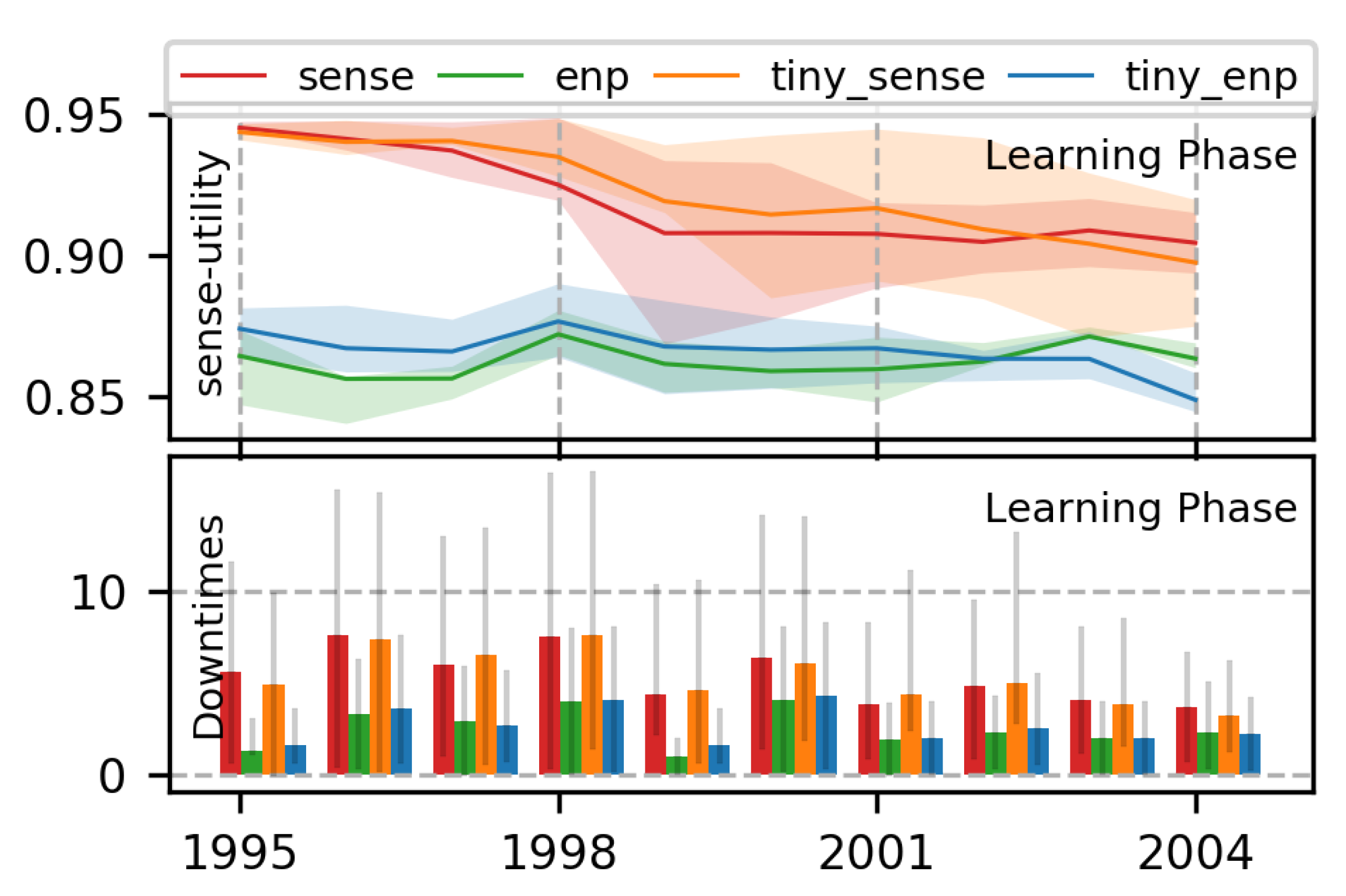
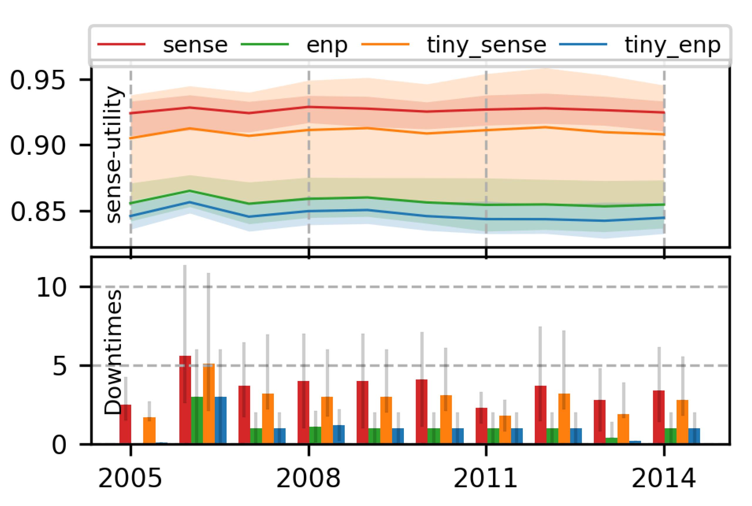
7.1.4. Effect of Size of NN

We also evaluate agents based on our MDP using a smaller NN. We do this to ensure that our results are superior because of our MDP and not simply because of a larger NN. We evaluate tiny_sense and tiny_enp with 64 nodes in their hidden layer (≈5 k parameters) that are otherwise identical to sense and enp agents which have 256 nodes (≈70 k parameters). We observe from Figure 15 and Figure 16 that the learning and testing behaviour of tiny_sense and tiny_enp do not differ significantly from that of sense and enp. This puts aside our suspicion that our solutions are superior just because we use a larger NN with more computation. The results from Figure 15 and Figure 16 indicate that it is possible to learn intelligent policies with small NNs and reduce computation resources required for RL-based solutions on the edge. However, a downside to using smaller NNs is the gradual loss in training stability (notice the large variation in sense-utility for tiny_sense during test in Figure 16 (top)). As we reduce the size of NN further, it becomes difficult to converge during learning. One way to compensate for the loss in learning stability would be to use specialized RL algorithms and NN architectures depending on the hardware platform and application scenario.

7.2. Runtime Tradeoffs

We now shift our discussion to how it may be possible to optimize runtime tradeoffs between two or more objectives over a space of preferences. We consider the dual-objective case where the single-task EHWSN agent has to optimize between maximizing the sense-utility $u_t^{sense}$, and the ENP-utility $u_t^{ENP}$. $\omega$ is the user-defined parameterized priority for sense-utility w.r.t. ENP-utility. The ultimate goal of the MORL agent is to maximize the node-utility, $w_t=\omega u_t^{sense}+(1-\omega )u_t^{ENP}$.

7.2.1. Limitations of Traditional Scalarization Methods

We first demonstrate the limitations of traditional RL methods that attempt to optimize over multiple objectives using scalarization. Figure 17 shows mul_scalar (purple) that scalarizes different objective rewards by multiplying them together as in [7,50,52]. Its reward function is $r=u^{sense}\times u^{ENP}$. This agent cannot tradeoff between sense-utility and ENP because its reward function is fixed and does not contain the $\omega$ parameter. The resulting policy is an “average” between maximizing sense-utility and ENP-utility and it is not clear how one can tweak the reward function with a single parameter to gradually bias the agent to optimize any one of the objectives.

add_scalar uses the reward values obtained by a linear combination of the different objective rewards weighted by their relative preferences [51,52]. For e.g., add_scalar(0.8) in Figure 17 uses a reward function defined by $r=\omega u^{sense}+(1-\omega )u^{ENP}$ where $\omega =0.8$. The resultant policy sacrifices energy neutrality (i.e., higher downtimes) for higher sense utility. Similarly, add_scalar(0.2) trades off sense-utility for lower downtimes (better ENP). By altering the value of $\omega$, the user can trade off between sense-utility and ENP. However, this method requires the user to fix the value of $\omega$ before training the RL agent. If the user requires a different $\omega$, the agent needs to be retrained with a new reward function corresponding to the new value of $\omega$. As a result, this method cannot be used to tradeoff during runtime. This is a major disadvantage because the parameter $\omega$ can change at every timestep. Thus, we can see that it is not possible for the user to tradeoff at runtime using traditional scalarization methods. We refer the reader to [52] for an in-depth analysis of different reward scalarization schemes for ENO.

7.2.2. Trading off with Runtime MORL (Algorithm 1)

We use Runtime MORL algorithm (Algorithm 1) in order to tradeoff between objectives at runtime by varying the parameter $\omega$. This is implemented as the morl_runtime($\omega$) agent. morl_runtime($\omega$) uses the actor-critic pairs from sense and enp agents to generate policies that can tradeoff at runtime.

In Figure 18, we compare between morl_runtime($\omega$) and add_scalar($\omega$) to analyze their tradeoff characteristics. We observe that our morl_runtime($\omega$) agent can indeed trade-off by varying $\omega$ at runtime without any retraining. High sense-priority ($\omega =0.8$, green) increases utility and downtimes and vice versa for low priority ($\omega =0.2$, red). We note that the range of tradeoffs is lesser for morl_runtime than add_scalar. This is because the tradeoff takes place in the value space for morl_runtime and in the reward space for add_scalar. Although the range of tradeoffs may be decreased in morl_runtime, it is more optimal. This can also be observed in Figure 18 where morl_runtime(0.2) (pink) consistently extracts much higher utility than add_scalar(0.2) (cyan) for similar energy-neutrality. Likewise, add_scalar(0.8) (orange) has disproportionately higher downtimes for only a slight increase in sense-utility than our morl_runtime(0.8) (green).

Thus, we see that our proposed Runtime MORL algorithm can generate better policies than scalarization methods that can tradeoff w.r.t. ω at runtime.

7.3. Learning Multi-Objective RL Policies for ENO

The previous results demonstrate how we can use Algorithm 1 for runtime tradeoffs using pre-trained greedy agent actor-critic pairs. We now consider a more realistic scenario for EWHSNs where we don’t have pre-trained greedy agents. The MORL agent has to learn these actors and critics tabula rasa and use them for runtime tradeoffs between different objectives. We consider the case for single-task EWHSN (two objectives) and dual-task EHWSN (three objectives). These are obviously harder learning problems that require efficient learning within a larger exploration space.

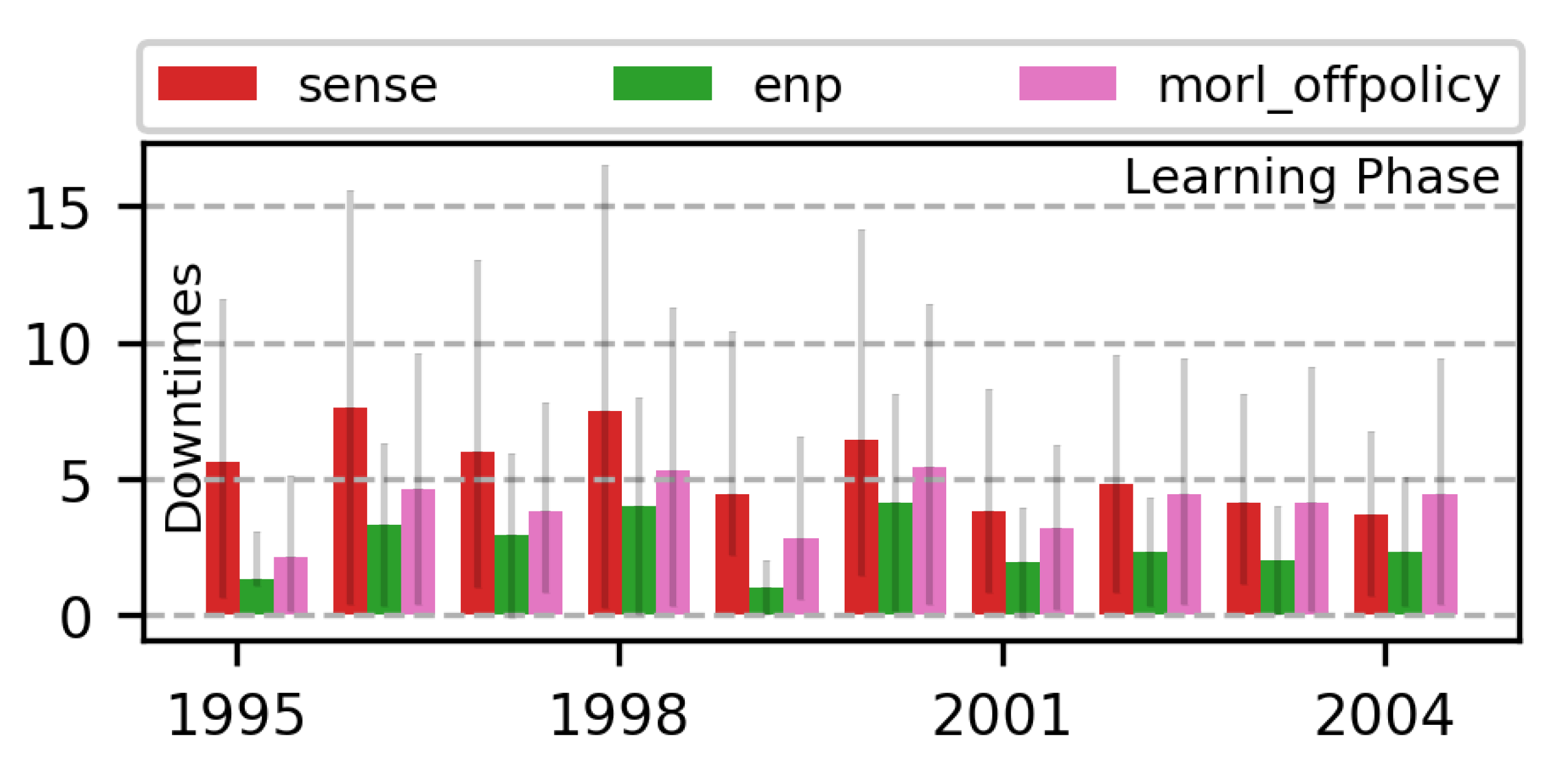
7.3.1. 2-Objective MOO with Off-Policy MORL (Algorithm 2)

We train a single-task EWHSN MORL agent, morl_offpolicy, that has to learn policies for runtime tradeoffs between two objectives (maximizing utility and minimizing downtimes). Figure 19 compares the test performance for morl_offpolicy($\omega$) for different values of the preference parameter $\omega$ against our baseline SORL agents sense and enp. morl_offpolicy learns the greedy actor-critics for both sense and ENO objectives and trades off between them using Algorithm 2. This is a difficult learning problem because morl_offpolicy has to learn two different actor-critic pairs, optimized for two different conflicting objectives using the same experience replay stream. Algorithm 2 achieves this by using off-policy corrections [75,76] (see Section 5.3). This is very different from the learning process of SORL agents like sense and enp where they learn using experience samples only for their respective objectives.

In Figure 19, it is clear that changing $\omega$ from 0.1 to 0.8 increases sensing utility with corresponding tradeoffs in energy neutrality. Both morl_offpolicy(0.1) and morl_offpolicy(0.8) (blue and brown bars) incur slightly higher losses (and higher variations) in energy neutrality compared to the sense and enp baselines (red and green bars). This is expected because morl_offpolicy uses the same amount of training as SORL baselines to learn a harder problem so there is a slight degradation in stability and optimality.

Figure 20 compares the cumulative learning costs between morl_offpolicy and traditional scalarization methods (add_scalar and mul_scalar). We observe that the gross learning cost of morl_offpolicy is not much higher than that of other methods. Thus, morl_offpolicy can learn a more difficult problem (i.e., multiple actor-critic policies that can tradeoff at runtime) with similar learning costs as previous methods.

We analyze the learning performance of morl_offpolicy in more detail in Figure 21 where we compare the learning costs (downtimes) between morl_offpolicy and SORL baseline agents. We observe that the learning costs are somewhere in between that of sense and enp. This is encouraging because this means we do not need exorbitant learning costs for a MORL policy using our framework. The reason for this efficient learning is as follows. During the early stages of training, the actor-critic pairs (like that of sense) are imperfect and prone to taking very extreme and potentially dangerous actions to maximize their objectives. For SORL agents with a single actor-critic pair, this results in large downtimes which increases the learning costs. Alternatively, actor-critic pairs which are optimized to minimize negative rewards (like enp) are too cautious, resulting in insufficient exploration, lost opportunities for maximization, and therefore converge to non-optimal policies. However, since morl_offpolicy has two actor-critic pairs that influence the exploration policy from two opposing directions (maximizing utility and minimizing downtimes), the final policy is a compromise between them that checks the agent from committing extreme actions that seem lucrative in the short term but are dangerous in the long run. Thus, even with imperfect actors and critics, the agent can avoid unsafe/non-optimal state-action spaces. Thus, with our method, the agent explores the state space in a safe manner and learns a harder problem more efficiently than traditional methods.

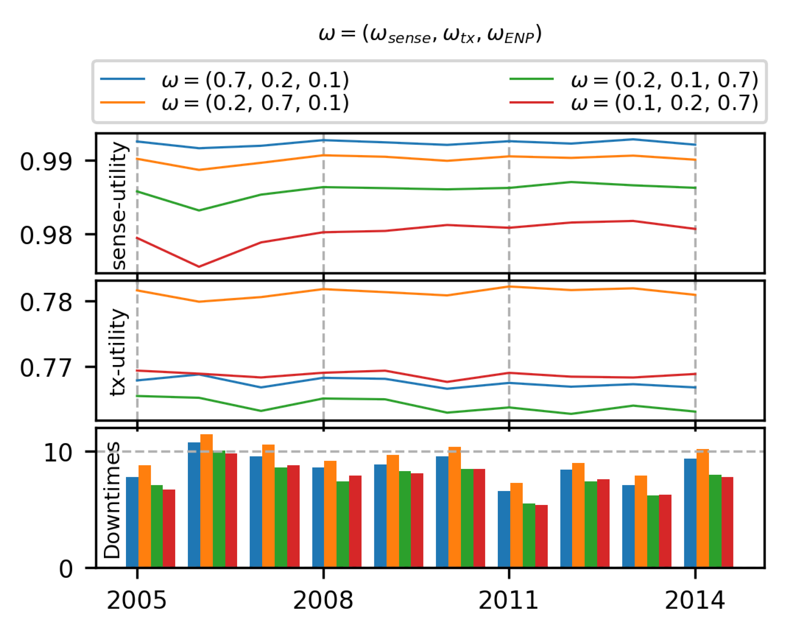
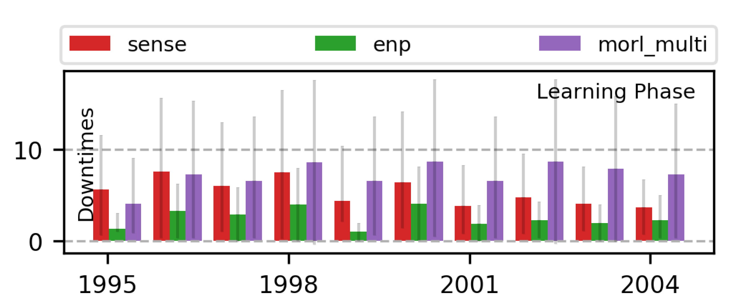
7.3.2. 3-Objective MOO with Off-Policy MORL (Algorithm 2)

Finally, we consider the case of the dual-task EHWSN. Here, the MORL agent has to learn policies that tradeoff between three objectives (maximizing sense-utility, maximizing transmission-utility, and minimizing downtimes). The tradeoffs are made at each timestep based on the user priority $\omega =({\omega }_{sense},{\omega }_{tx},{\omega }_{ENP})$. We train the morl_multi agent using Algorithm 2. We use the same discount factors for all tasks (to simplify analysis). The action space is two-dimensional in this case and so the convex hull is a 2-D polygon from which potentially optimal actions are sampled. During testing, we compare the performance of morl_multi for different values of constant $\omega$. We observe whether the results policies can maximize the different objectives and tradeoff w.r.t. $\omega$.

In Figure 22, we first observe how morl_multi trades off its energy neutrality with changing $\omega$. When energy neutrality has low priority (${\omega }_{ENP}=0.1$, blue and orange), the downtimes (bottom bar plot) are much higher than when ${\omega }_{ENP}=0.7$ (green and red). As a result of this trade off, the corresponding utilities for ${\omega }_{ENP}=0.1$ are much higher than that of ${\omega }_{ENP}=0.7$ (top and middle figures).

Secondly, we observe how the agent trades off between sense-utility and tx-utility. Let us consider two cases where the ENO objective has the same preference i.e., ${\omega }_{ENP}=0.1$ (blue and orange). The blue line corresponds to a higher preference for sensing than for transmission (i.e., ${\omega }_{sense}>{\omega }_{tx}$) and vice versa for the orange line. Thus, the blue line scores higher in sense-utility than the orange line (top figure). However, it scores lower in tx-utility compared to the orange line (middle figure). A similar observation can be made when ${\omega }_{ENP}=0.7$ (green and red lines). This clearly demonstrates that morl_multi can trade-off between its different objectives.

Thirdly, we analyze the tradeoff between sensing-utility and ENP. In the top figure of Figure 22, we observe that as we progressively decrease the priority for sensing and increase the priority for energy neutrality, the agent decreases its sense-utility and downtimes correspondingly (blue → orange → green → red) i.e., it becomes more energy-neutral at the expense of lower utility. A similar trend can be observed in the middle figure for tx-utility (orange → blue → red → green). However due to the concavity of the tx-utility, there is a larger drop when the tx-priority ${\omega }_{tx}$ is reduced from $0.7$ to $0.2$. The tradeoff between sensing-utility and ENP is very clear when we observe the blue and red lines/bars. Both the blue and red lines correspond to ${\omega }_{tx}=0.2$ and so their tx-utility is very similar (middle figure). However, the blue line corresponding to ${\omega }_{sense}>{\omega }_{ENP}$ has a much higher sense-utility (see top figure) than the red line (${\omega }_{sense}<{\omega }_{ENP}$) at the expense of higher downtimes (see bottom figure).

Finally, we discuss the learning costs for morl_multi shown in Figure 23. We observe that it has an acceptable number of average downtimes (less than 15) during testing and learning, which is competitive with previous methods [8]. This means that morl_multi policies are stable, convergent, and energy neutral in spite of having to learn three different greedy actor-critics within the same training period as previous methods. This is primarily due to off-policy corrections in Algorithm 2 and safe exploration induced by safe actions as well as auto-regulation among the greedy agents. Thus, our framework can learn to optimize between three objectives successfully in dual-task EHWSNs, without a drastic increase in learning costs, which indicates that it can be scaled to any number of tasks as required. With additional tasks, their convex hull formed by greedy actions will have correspondingly more dimensions. This means that we will have to sample and evaluate more actions from this hull which increases the computational requirements. One can compensate for this through a more coarse-grained sampling of actions at the expense of fewer optimal solutions.

From the above observations and analysis, we show that our proposed MORL framework for ENO of EHWSNs is not only feasible but also superior to previous methods. We can learn more optimal policies with lower learning costs and tradeoffs at runtime. This can be attributed to our more appropriate MDP formulation of the ENO problem. Also, by compromising between compute-intensive MORL methods and elitist MC/EA methods, our proposed MORL algorithms are a feasible solution for resource-constrained EHWSN.

8. Conclusions and Future Directions

IoT embedded systems require MOO to coordinate and optimize its limited resource among multiple tasks. Traditional heuristics (like MC roll-outs, EA) are unsuited for this because they assume time-invariant objective functions whereas node-level MOO generally requires time-varying objective functions. Other alternative methods either result in non-optimal solutions or have very high computation costs making them unsuitable for embedded systems.

We provide a MORL framework for MOO in IoT embedded devices in order to overcome this problem. The framework is made up of general MOMDP and two low-compute MORL algorithms. These algorithms offer a workable solution for resource-constrained EHWSNs by falling somewhere between non-adaptive heuristics and compute-intensive MORL approaches. With our proposed framework, embedded devices can learn to make tradeoffs while maintaining reasonable learning costs. We use single-task and dual-task EHWSNs as an example application and demonstrate MOO for ENO. We create an appropriate MOMDP for the EHWSN system model and assess the performance of our suggested algorithms. Our findings demonstrate that adopting our framework allows for the run-time tradeoff of objectives and the learning of near-optimal policies at lower learning costs.

Our MORL solution still needs to be improved to be implemented in IoT systems with severe resource constraints. Since our framework can theoretically be applied to other less compute-intensive RL algorithms, some alternatives to DDPG include using tabular approaches [7,9], linear function approximation [6,11,50], or distributed learning [8]. In our other paper [8], we show that inefficient exploration is one of the major causes of such instability and propose a distributed RL method with novel $ϵ$-greedy exploration strategies to not only minimize the learning time and computational costs. This is orthogonal to this work and can be combined together to get more powerful policies at lower learning costs.

Another strategy to implement MORL NN models in IoT embedded devices would be to compress the NN model. Recent works have shown that it is possible to compress a large 16 GB ImageNet model and fit it into a micro-controller [77] without compromising too much on accuracy and latency. Encouraging results have been reported in [78] where the authors implement Deep RL to optimize the modulation scheme for software-defined radio in real-time low-power hardware.

References

1. Ma, D.; Lan, G.; Hassan, M.; Hu, W.; Das, S.K. Sensing, Computing, and Communications for Energy Harvesting IoTs: A Survey. IEEE Commun. Surv. Tutor. 2019, 22, 1222–1250. [Google Scholar] [CrossRef]
2. Nakamura, Y.; Arakawa, Y.; Kanehira, T.; Fujiwara, M.; Yasumoto, K. Senstick: Comprehensive sensing platform with an ultra tiny all-in-one sensor board for iot research. J. Sens. 2017, 2017, 6308302. [Google Scholar] [CrossRef] [Green Version]
3. Vamplew, P.; Yearwood, J.; Dazeley, R.; Berry, A. On the limitations of scalarisation for multi-objective reinforcement learning of pareto fronts. In Proceedings of the Australasian Joint Conference on Artificial Intelligence, Auckland, New Zealand, 1–5 December 2008; Springer: Berlin/Heidelberg, Germany, 2008; pp. 372–378. [Google Scholar]
4. Sutton, R.S.; Barto, A.G. Reinforcement Learning: An Introduction; MIT Press: Cambridge, MA, USA, 2018. [Google Scholar]
5. Blasco, P.; Gunduz, D.; Dohler, M. A learning theoretic approach to energy harvesting communication system optimization. IEEE Trans. Wirel. Commun. 2013, 12, 1872–1882. [Google Scholar] [CrossRef] [Green Version]
6. Ortiz, A.; Al-Shatri, H.; Li, X.; Weber, T.; Klein, A. Reinforcement learning for energy harvesting point-to-point communications. In Proceedings of the 2016 IEEE International Conference on Communications (ICC), Kuala Lumpur, Malaysia, 22–27 May 2016; pp. 1–6. [Google Scholar]
7. Hsu, R.C.; Liu, C.T.; Wang, H.L. A reinforcement learning-based ToD provisioning dynamic power management for sustainable operation of energy harvesting wireless sensor node. IEEE Trans. Emerg. Top. Comput. 2014, 2, 181–191. [Google Scholar] [CrossRef]
8. Shresthamali, S.; Kondo, M.; Nakamura, H. Power Management of Wireless Sensor Nodes with Coordinated Distributed Reinforcement Learning. In Proceedings of the 2019 IEEE 37th International Conference on Computer Design (ICCD), Abu Dhabi, United Arab Emirates, 17–20 November 2019; pp. 638–647. [Google Scholar]
9. Shresthamali, S.; Kondo, M.; Nakamura, H. Adaptive power management in solar energy harvesting sensor node using reinforcement learning. ACM Trans. Embed. Comput. Syst. (TECS) 2017, 16, 181. [Google Scholar] [CrossRef]
10. Fraternali, F.; Balaji, B.; Agarwal, Y.; Gupta, R.K. ACES–Automatic Configuration of Energy Harvesting Sensors with Reinforcement Learning. arXiv 2019, arXiv:1909.01968. [Google Scholar]
11. Sawaguchi, S.; Christmann, J.F.; Lesecq, S. Highly adaptive linear actor-critic for lightweight energy-harvesting IoT applications. J. Low Power Electron. Appl. 2021, 11, 17. [Google Scholar] [CrossRef]
12. Parisi, S.; Pirotta, M.; Smacchia, N.; Bascetta, L.; Restelli, M. Policy gradient approaches for multi-objective sequential decision making. In Proceedings of the 2014 International Joint Conference on Neural Networks (IJCNN), Beijing, China, 6–11 July 2014; pp. 2323–2330. [Google Scholar]
13. Pirotta, M.; Parisi, S.; Restelli, M. Multi-objective reinforcement learning with continuous pareto frontier approximation. In Proceedings of the Twenty-Ninth AAAI Conference on Artificial Intelligence, Austin, TX, USA, 25–30 January 2015. [Google Scholar]
14. Yang, R.; Sun, X.; Narasimhan, K. A generalized algorithm for multi-objective reinforcement learning and policy adaptation. In Proceedings of the Advances in Neural Information Processing Systems, Vancouver, BC, Canada, 8–14 December 2019; pp. 14636–14647. [Google Scholar]
15. Mnih, V.; Kavukcuoglu, K.; Silver, D.; Rusu, A.A.; Veness, J.; Bellemare, M.G.; Graves, A.; Riedmiller, M.; Fidjeland, A.K.; Ostrovski, G.; et al. Human-level control through deep reinforcement learning. Nature 2015, 518, 529. [Google Scholar] [CrossRef]
16. Silver, D.; Huang, A.; Maddison, C.J.; Guez, A.; Sifre, L.; Van Den Driessche, G.; Schrittwieser, J.; Antonoglou, I.; Panneershelvam, V.; Lanctot, M.; et al. Mastering the game of Go with deep neural networks and tree search. Nature 2016, 529, 484. [Google Scholar] [CrossRef]
17. Sudevalayam, S.; Kulkarni, P. Energy harvesting sensor nodes: Survey and implications. IEEE Commun. Surv. Tutor. 2011, 13, 443–461. [Google Scholar] [CrossRef] [Green Version]
18. Kansal, A.; Hsu, J.; Zahedi, S.; Srivastava, M.B. Power management in energy harvesting sensor networks. ACM Trans. Embed. Comput. Syst. 2007, 6, 32. [Google Scholar] [CrossRef]
19. Shresthamali, S.; Kondo, M.; Nakamura, H. Multi-objective Reinforcement Learning for Energy Harvesting Wireless Sensor Nodes. In Proceedings of the 2021 IEEE 14th International Symposium on Embedded Multicore/Many-core Systems-on-Chip (MCSoC), Singapore, 20–23 December 2021; pp. 98–105. [Google Scholar]
20. Vigorito, C.M.; Ganesan, D.; Barto, A.G. Adaptive control of duty cycling in energy-harvesting wireless sensor networks. In Proceedings of the 2007 4th Annual IEEE Communications Society Conference on Sensor, Mesh and Ad Hoc Communications and Networks, San Francisco, CA, USA, 18–21 June 2007; pp. 21–30. [Google Scholar]
21. Sharma, V.; Mukherji, U.; Joseph, V.; Gupta, S. Optimal energy management policies for energy harvesting sensor nodes. IEEE Trans. Wirel. Commun. 2010, 9, 1326–1336. [Google Scholar] [CrossRef] [Green Version]
22. Ozel, O.; Tutuncuoglu, K.; Yang, J.; Ulukus, S.; Yener, A. Transmission with energy harvesting nodes in fading wireless channels: Optimal policies. IEEE J. Sel. Areas Commun. 2011, 29, 1732–1743. [Google Scholar] [CrossRef] [Green Version]
23. Peng, S.; Low, C. Prediction free energy neutral power management for energy harvesting wireless sensor nodes. Ad Hoc Netw. 2014, 13, 351–367. [Google Scholar] [CrossRef]
24. Cionca, V.; McGibney, A.; Rea, S. MAllEC: Fast and Optimal Scheduling of Energy Consumption for Energy Harvesting Devices. IEEE Internet Things J. 2018, 5, 5132–5140. [Google Scholar] [CrossRef]
25. Jia, R.; Zhang, J.; Liu, X.Y.; Liu, P.; Fu, L.; Wang, X. Optimal Rate Control for Energy-Harvesting Systems with Random Data and Energy Arrivals. ACM Trans. Sens. Netw. 2019, 15, 13. [Google Scholar] [CrossRef]
26. Fu, A.; Modiano, E.; Tsitsiklis, J.N. Optimal transmission scheduling over a fading channel with energy and deadline constraints. IEEE Trans. Wirel. Commun. 2006, 5, 630–641. [Google Scholar] [CrossRef]
27. Lei, L.; Kuang, Y.; Shen, X.S.; Yang, K.; Qiao, J.; Zhong, Z. Optimal reliability in energy harvesting industrial wireless sensor networks. IEEE Trans. Wirel. Commun. 2016, 15, 5399–5413. [Google Scholar] [CrossRef] [Green Version]
28. Buchli, B.; Sutton, F.; Beutel, J.; Thiele, L. Dynamic power management for long-term energy neutral operation of solar energy harvesting systems. In Proceedings of the 12th ACM Conference on Embedded Network Sensor Systems, Memphis, TN, USA, 3–6 November 2014; pp. 31–45. [Google Scholar]
29. Geissdoerfer, K.; Jurdak, R.; Kusy, B.; Zimmerling, M. Getting more out of energy-harvesting systems: Energy management under time-varying utility with PreAct. In Proceedings of the 18th International Conference on Information Processing in Sensor Networks, Montreal, QC, Canada, 16–18 April 2019; pp. 109–120. [Google Scholar]
30. Mao, S.; Cheung, M.H.; Wong, V.W. Joint energy allocation for sensing and transmission in rechargeable wireless sensor networks. IEEE Trans. Veh. Technol. 2014, 63, 2862–2875. [Google Scholar] [CrossRef] [Green Version]
31. GhasemAghaei, R.; Rahman, M.A.; Gueaieb, W.; El Saddik, A. Ant colony-based reinforcement learning algorithm for routing in wireless sensor networks. In Proceedings of the Instrumentation and Measurement Technology Conference Proceedings, IMTC 2007, Warsaw, Poland, 1–3 May 2007; pp. 1–6. [Google Scholar]
32. Blasco, P.; Gündüz, D. Multi-access communications with energy harvesting: A multi-armed bandit model and the optimality of the myopic policy. IEEE J. Sel. Areas Commun. 2015, 33, 585–597. [Google Scholar] [CrossRef] [Green Version]
33. Chan, W.H.R.; Zhang, P.; Nevat, I.; Nagarajan, S.G.; Valera, A.C.; Tan, H.X.; Gautam, N. Adaptive duty cycling in sensor networks with energy harvesting using continuous-time Markov chain and fluid models. IEEE J. Sel. Areas Commun. 2015, 33, 2687–2700. [Google Scholar] [CrossRef]
34. Xiao, Y.; Han, Z.; Niyato, D.; Yuen, C. Bayesian reinforcement learning for energy harvesting communication systems with uncertainty. In Proceedings of the Communications (ICC), 2015 IEEE International Conference on, London, UK, 8–12 June 2015; pp. 5398–5403. [Google Scholar]
35. Mihaylov, M.; Tuyls, K.; Nowé, A. Decentralized learning in wireless sensor networks. In Proceedings of the International Workshop on Adaptive and Learning Agents, Budapest, Hungary, 12 May 2009; Springer: Berlin/Heidelberg, Germany, 2009; pp. 60–73. [Google Scholar]
36. Hsu, J.; Zahedi, S.; Kansal, A.; Srivastava, M.; Raghunathan, V. Adaptive duty cycling for energy harvesting systems. In Proceedings of the 2006 ISLPED, Bavaria, Germany, 4–6 October 2006; pp. 180–185. [Google Scholar]
37. OpenAI. Faulty Reward Functions in the Wild. 2020. Available online: https://openai.com/blog/faulty-reward-functions/ (accessed on 4 July 2020).
38. DeepMind. Designing Agent Incentives to Avoid Reward Tampering. 2020. Available online: https://deepmindsafetyresearch.medium.com/designing-agent-incentives-to-avoid-reward-tampering-4380c1bb6cd (accessed on 4 July 2020).
39. Everitt, T.; Hutter, M. Reward Tampering Problems and Solutions in Reinforcement Learning: A Causal Influence Diagram Perspective. arXiv 2019, arXiv:1908.04734. [Google Scholar] [CrossRef]
40. Xu, Y.; Lee, H.G.; Tan, Y.; Wu, Y.; Chen, X.; Liang, L.; Qiao, L.; Liu, D. Tumbler: Energy Efficient Task Scheduling for Dual-Channel Solar-Powered Sensor Nodes. In Proceedings of the 56th Annual Design Automation Conference 2019 (DAC’19), Las Vegas, NV, USA, 2–6 June 2019; ACM: New York, NY, USA, 2019; pp. 172:1–172:6. [Google Scholar] [CrossRef]
41. Gai, K.; Qiu, M. Optimal resource allocation using reinforcement learning for IoT content-centric services. Appl. Soft Comput. 2018, 70, 12–21. [Google Scholar] [CrossRef]
42. Xu, Y.; Lee, H.G.; Chen, X.; Peng, B.; Liu, D.; Liang, L. Puppet: Energy Efficient Task Mapping For Storage-Less and Converter-Less Solar-Powered Non-Volatile Sensor Nodes. In Proceedings of the 2018 IEEE 36th International Conference on Computer Design (ICCD), Orlando, FL, USA, 7–10 October 2018; pp. 226–233. [Google Scholar]
43. Dias, G.M.; Nurchis, M.; Bellalta, B. Adapting sampling interval of sensor networks using on-line reinforcement learning. In Proceedings of the 2016 IEEE 3rd World Forum on Internet of Things (WF-IoT), Reston, VA, USA, 12–14 December 2016; pp. 460–465. [Google Scholar]
44. Murad, A.; Kraemer, F.A.; Bach, K.; Taylor, G. Autonomous Management of Energy-Harvesting IoT Nodes Using Deep Reinforcement Learning. arXiv 2019, arXiv:1905.04181. [Google Scholar]
45. Ortiz Jimenez, A.P. Optimization and Learning Approaches for Energy Harvesting Wireless Communication Systems. Ph.D. Thesis, Technische Universität, Darmstadt, Germany, 2019. [Google Scholar]
46. Qiu, C.; Hu, Y.; Chen, Y.; Zeng, B. Deep deterministic policy gradient (DDPG)-based energy harvesting wireless communications. IEEE Internet Things J. 2019, 6, 8577–8588. [Google Scholar] [CrossRef]
47. Kim, H.; Shin, W.; Yang, H.; Lee, N.; Lee, J. Rate Maximization with Reinforcement Learning for Time-Varying Energy Harvesting Broadcast Channels. In Proceedings of the 2019 IEEE Global Communications Conference (GLOBECOM), Big Island, HI, USA, 9–13 December 2019; pp. 1–6. [Google Scholar]
48. Van Huynh, N.; Hoang, D.T.; Nguyen, D.N.; Dutkiewicz, E.; Niyato, D.; Wang, P. Optimal and Low-Complexity Dynamic Spectrum Access for RF-Powered Ambient Backscatter System with Online Reinforcement Learning. IEEE Trans. Commun. 2019, 67, 5736–5752. [Google Scholar] [CrossRef] [Green Version]
49. Long, J.; Büyüköztürk, O. Collaborative duty cycling strategies in energy harvesting sensor networks. Comput. Aided Civ. Infrastruct. Eng. 2020, 35, 534–548. [Google Scholar] [CrossRef]
50. Aoudia, F.A.; Gautier, M.; Berder, O. RLMan: An energy manager based on reinforcement learning for energy harvesting wireless sensor networks. IEEE Trans. Green Commun. Netw. 2018, 2, 408–417. [Google Scholar] [CrossRef] [Green Version]
51. Ferreira, P.V.R.; Paffenroth, R.; Wyglinski, A.M.; Hackett, T.M.; Bilén, S.G.; Reinhart, R.C.; Mortensen, D.J. Multiobjective reinforcement learning for cognitive satellite communications using deep neural network ensembles. IEEE J. Sel. Areas Commun. 2018, 36, 1030–1041. [Google Scholar] [CrossRef]
52. Rioual, Y.; Le Moullec, Y.; Laurent, J.; Khan, M.I.; Diguet, J.P. Reward Function Evaluation in a Reinforcement Learning Approach for Energy Management. In Proceedings of the 2018 16th Biennial Baltic Electronics Conference (BEC), Tallinn, Estonia, 8–10 October 2018; pp. 1–4. [Google Scholar]
53. Liu, C.; Xu, X.; Hu, D. Multiobjective reinforcement learning: A comprehensive overview. IEEE Trans. Syst. Man, Cybern. Syst. 2014, 45, 385–398. [Google Scholar]
54. Zeng, F.; Zong, Q.; Sun, Z.; Dou, L. Self-adaptive multi-objective optimization method design based on agent reinforcement learning for elevator group control systems. In Proceedings of the 2010 8th World Congress on Intelligent Control and Automation, Jinan, China, 6–9 July 2010; pp. 2577–2582. [Google Scholar]
55. Ngai, D.C.K.; Yung, N.H.C. A multiple-goal reinforcement learning method for complex vehicle overtaking maneuvers. IEEE Trans. Intell. Transp. Syst. 2011, 12, 509–522. [Google Scholar] [CrossRef] [Green Version]
56. Moffaert, K.V.; Nowé, A. Multi-Objective Reinforcement Learning using Sets of Pareto Dominating Policies. J. Mach. Learn. Res. 2014, 15, 3663–3692. [Google Scholar]
57. Shelton, C.R. Importance Sampling for Reinforcement Learning with Multiple Objectives. Ph.D. Thesis, MIT, Cambridge, MA, USA, 2001. [Google Scholar]
58. Li, K.; Zhang, T.; Wang, R. Deep reinforcement learning for multiobjective optimization. IEEE Trans. Cybern. 2020, 51, 3103–3114. [Google Scholar] [CrossRef] [PubMed]
59. Lillicrap, T.P.; Hunt, J.J.; Pritzel, A.; Heess, N.; Erez, T.; Tassa, Y.; Silver, D.; Wierstra, D. Continuous control with deep reinforcement learning. arXiv 2015, arXiv:1509.02971. [Google Scholar]
60. Yang, Z.; Merrick, K.E.; Abbass, H.A.; Jin, L. Multi-Task Deep Reinforcement Learning for Continuous Action Control. In Proceedings of the IJCAI, Melbourne, Australia, 19–25 August 2017; pp. 3301–3307. [Google Scholar]
61. Li, C.; Czarnecki, K. Urban Driving with Multi-Objective Deep Reinforcement Learning. arXiv 2019, arXiv:1811.08586. [Google Scholar]
62. Sharma, M.K.; Zappone, A.; Assaad, M.; Debbah, M.; Vassilaras, S. Distributed power control for large energy harvesting networks: A multi-agent deep reinforcement learning approach. IEEE Trans. Cogn. Commun. Netw. 2019, 5, 1140–1154. [Google Scholar] [CrossRef]
63. Ortiz, A.; Al-Shatri, H.; Weber, T.; Klein, A. Multi-Agent Reinforcement Learning for Energy Harvesting Two-Hop Communications with a Partially Observable State. arXiv 2017, arXiv:1702.06185. [Google Scholar] [CrossRef]
64. Jia, J.; Chen, J.; Chang, G.; Tan, Z. Energy efficient coverage control in wireless sensor networks based on multi-objective genetic algorithm. Comput. Math. Appl. 2009, 57, 1756–1766. [Google Scholar] [CrossRef] [Green Version]
65. Le Berre, M.; Hnaien, F.; Snoussi, H. Multi-objective optimization in wireless sensors networks. In Proceedings of the ICM 2011 Proceeding, Istanbul, Turkey, 13–15 April 2011; pp. 1–4. [Google Scholar]
66. Marks, M. A survey of multi-objective deployment in wireless sensor networks. J. Telecommun. Inf. Technol. 2010, 3, 36–41. [Google Scholar]
67. Fei, Z.; Li, B.; Yang, S.; Xing, C.; Chen, H.; Hanzo, L. A survey of multi-objective optimization in wireless sensor networks: Metrics, algorithms, and open problems. IEEE Commun. Surv. Tutor. 2016, 19, 550–586. [Google Scholar] [CrossRef] [Green Version]
68. Iqbal, M.; Naeem, M.; Anpalagan, A.; Ahmed, A.; Azam, M. Wireless sensor network optimization: Multi-objective paradigm. Sensors 2015, 15, 17572–17620. [Google Scholar] [CrossRef]
69. Konstantinidis, A.; Yang, K.; Zhang, Q. An evolutionary algorithm to a multi-objective deployment and power assignment problem in wireless sensor networks. In Proceedings of the IEEE GLOBECOM 2008—2008 IEEE Global Telecommunications Conference, New Orleans, LA, USA, 30 November–4 December 2008; pp. 1–6. [Google Scholar]
70. Ahmed, M.M.; Houssein, E.H.; Hassanien, A.E.; Taha, A.; Hassanien, E. Maximizing lifetime of large-scale wireless sensor networks using multi-objective whale optimization algorithm. Telecommun. Syst. 2019, 72, 243–259. [Google Scholar] [CrossRef]
71. Jia, J.; Chen, J.; Chang, G.; Wen, Y.; Song, J. Multi-objective optimization for coverage control in wireless sensor network with adjustable sensing radius. Comput. Math. Appl. 2009, 57, 1767–1775. [Google Scholar] [CrossRef] [Green Version]
72. Giardino, M.; Schwyn, D.; Ferri, B.; Ferri, A. Low-Overhead Reinforcement Learning-Based Power Management Using 2QoSM. J. Low Power Electron. Appl. 2022, 12, 29. [Google Scholar] [CrossRef]
73. Japan Meteorological Agency. Japan Meteorological Agency. 2019. Available online: https://www.jma.go.jp/jma/menu/menureport.html (accessed on 6 July 2019).
74. Libelium. Waspmote-The Sensor Platform to Develop IoT Projects. Available online: https://www.libelium.com/iot-products/waspmote/ (accessed on 22 January 2021).
75. Fujimoto, S.; Meger, D.; Precup, D. Off-policy deep reinforcement learning without exploration. In Proceedings of the International Conference on Machine Learning. PMLR, Long Beach, CA, USA, 9–15 June 2019; pp. 2052–2062. [Google Scholar]
76. Kumar, A.; Fu, J.; Tucker, G.; Levine, S. Stabilizing off-policy q-learning via bootstrapping error reduction. arXiv 2019, arXiv:1906.00949. [Google Scholar]
77. Lin, J.; Chen, W.M.; Lin, Y.; Cohn, J.; Gan, C.; Han, S. Mcunet: Tiny deep learning on iot devices. arXiv 2020, arXiv:2007.10319. [Google Scholar]
78. Restuccia, F.; Melodia, T. DeepWiERL: Bringing Deep Reinforcement Learning to the Internet of Self-Adaptive Things. In Proceedings of the IEEE INFOCOM 2020—IEEE Conference on Computer Communications, Toronto, ON, Canada, 6–9 July 2020; pp. 844–853. [Google Scholar]
Figure 1. A multi-task EHWSN has to wisely determine its gross energy consumption at each time step so as to remain energy-neutral. Furthermore, it has to proportion the energy among different tasks to maximize node utility.
Jlpea 12 00053 g001
Figure 2. A general system model for multi-task EHWSNs.
Jlpea 12 00053 g002
Figure 3. The Pareto-front changes when the agent transitions from state s 1 to s 2 . Crosses indicate Pareto-dominated actions. The marker size represents the utility of the action.
Jlpea 12 00053 g003
Figure 4. As we move from one greedy action to another in the action space, we traverse along the Pareto-optimal frontier in the objective space. Runtime MORL samples actions (red crosses) from in between the greedy actions, g 1 and g E N P .
Jlpea 12 00053 g004
Figure 5. Linear and concave reward functions quantify the utilities for different tasks such as sensing, communication, and processing. The ENP-utility function indicates the long-term energy neutrality of the node.
Jlpea 12 00053 g005
Figure 6. Agent enp (ours, green) has similar energy neutrality (downtimes) as the most energy-neutral policy max_enp. sense (ours, red) sacrifices some of its energy neutrality to increase its utility but is more energy neutral than max_k.
Jlpea 12 00053 g006
Figure 7. max_enp Heuristic Policy. The conformity of the node decreases gradually as the battery depletes.
Jlpea 12 00053 g007
Figure 8. Battery traces for sense, enp. sense is more aggressive than enp when maximizing the sense-utility and therefore experiences downtime during winter. The sharp rise in battery level after a downtime signifies a node reset.
Jlpea 12 00053 g008
Figure 9. bad_batt learns to accommodate for battery inefficiencies by maximizing duty cycles during the day. sense maximizes its duty cycle during the night depending on how much energy it was able to harvest during the day.
Jlpea 12 00053 g009
Figure 10. SORL methods can adapt to changes in working parameters.
Jlpea 12 00053 g010
Figure 11. Including temporal information in the state definition of enp (ours) decreases the downtimes during learning as compared to pomdp_enp (traditional MDPs).
Jlpea 12 00053 g011
Figure 12. enp (ours) learns to discriminate between aliased states using temporal information.
Jlpea 12 00053 g012
Figure 13. Our safe action definition (sense and enp) prevents over-provisioning and reduces the learning costs compared to traditional MDP definitions (raw_sense and raw_enp).
Jlpea 12 00053 g013
Figure 14. sense and enp learn using safe action definitions which result in robust and intelligent policies. Consequently during the test phase, sense and enp score much higher utilities at much lower downtimes compared to traditional solutions (raw_sense and raw_enp).
Jlpea 12 00053 g014
Figure 15. Learning performance of agents with smaller networks.
Jlpea 12 00053 g015
Figure 16. Test performance of agents with smaller networks.
Jlpea 12 00053 g016
Figure 17. Scalarization methods for MORL: add_scalar can tradeoff only if the relative priorities are known before training. It is not clear what objective mul_scalar is optimizing.
Jlpea 12 00053 g017
Figure 18. morl_runtime( ω ) (Algorithm 1) can tradeoff sense-utility with energy neutrality (downtimes) at runtime.
Jlpea 12 00053 g018
Figure 19. morl_offpolicy ( ω ) learns greedy actor-critics that can tradeoff between sense and ENO objectives using Algorithm 2.
Jlpea 12 00053 g019
Figure 20. morl_diff has learning costs comparable to other scalarization methods in spite of a harder learning problem.
Jlpea 12 00053 g020
Figure 21. morl_offpolicy has lower learning costs compared to sense and enp. This is because the opposing greedy actor-critics for MORL check each other from committing extreme actions.
Jlpea 12 00053 g021
Figure 22. morl_multi agent has lower downtimes when ENO has higher priority (green and red) than when it is lower (blue and orange). Given the same ω E N P , the agent trades off between sense-utility and tx-utility using the values of ω s e n s e and ω t x .
Jlpea 12 00053 g022
Figure 23. morl_multi has acceptable learning costs (slightly higher than sense) even though the learning problem is much harder.
Jlpea 12 00053 g023