
Real-Time Embedded Implementation of Improved Object Detector for Resource-Constrained Devices


Abstract
:1. Introduction
2. Background and Literature Review
2.1. Object Detectors
2.2. Bounding Box Regression Loss
2.3. Performance Metrics
- True positive (TP): correct prediction matching ground truth coordinates.
- False positive (FP): incorrect or misplaced detection of an object.
- False Negative (FN): undetected ground truth coordinates.
- True Negative (TN): prediction when no ground truth exists.
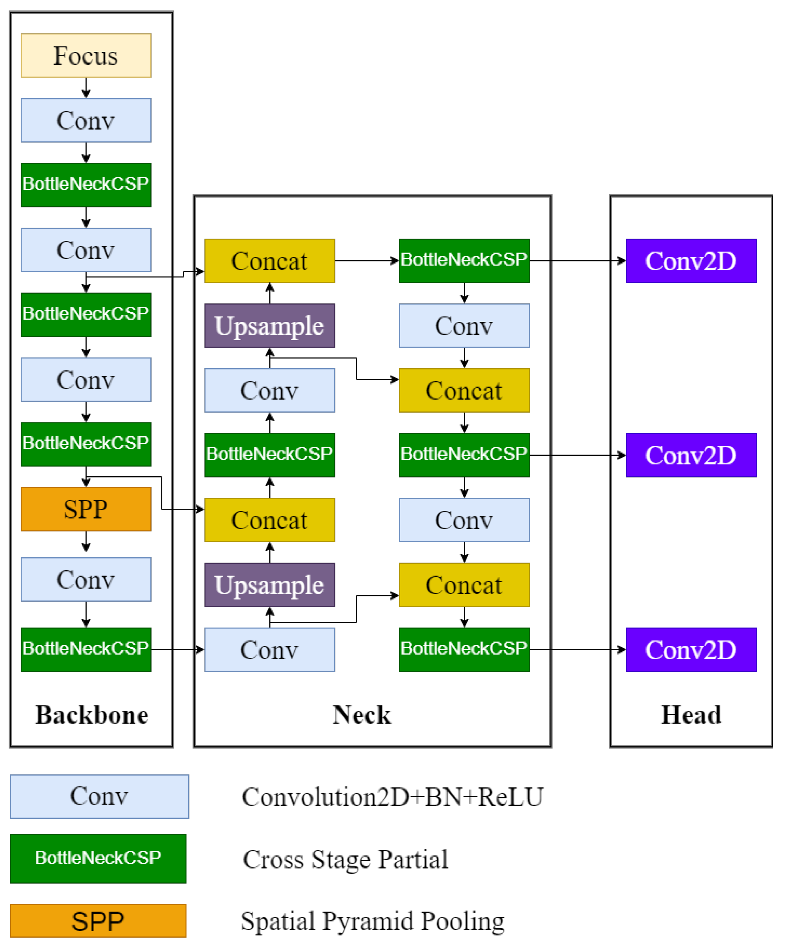
3. YOLO
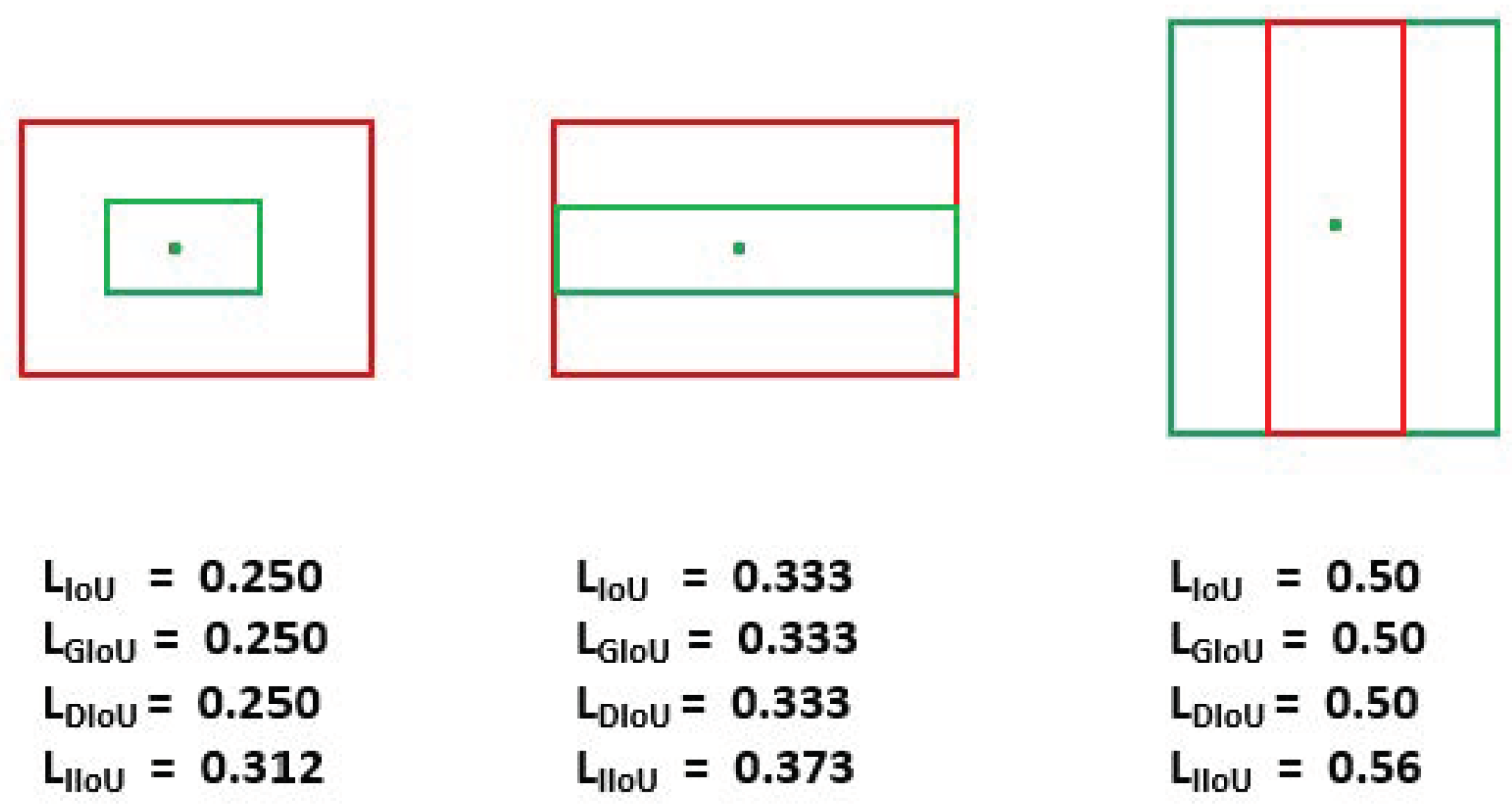
4. IoU Loss Metrics
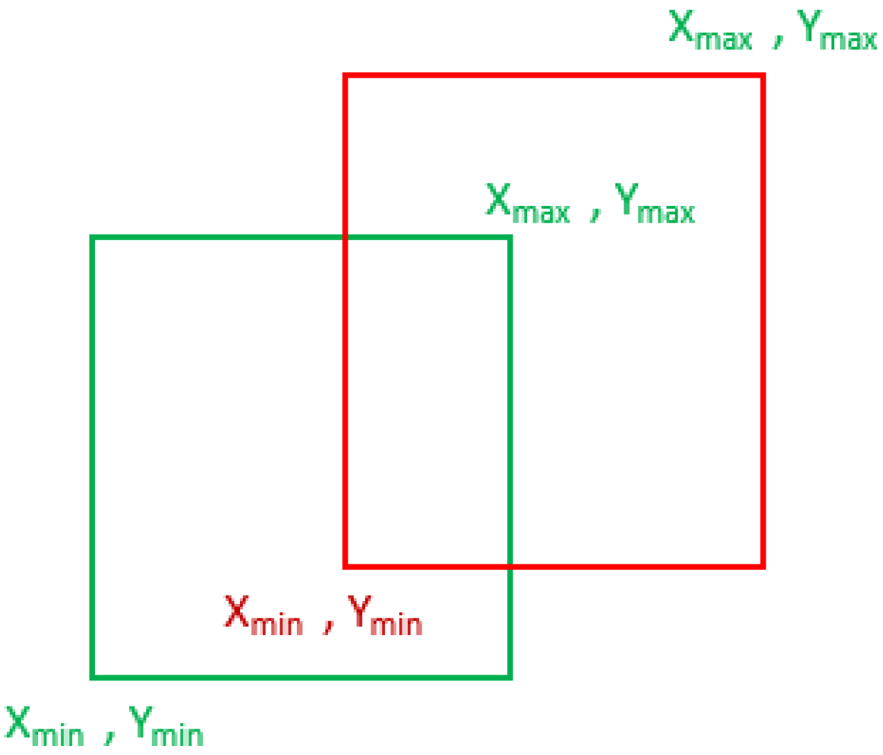
4.1. Intersection over Union (IoU)
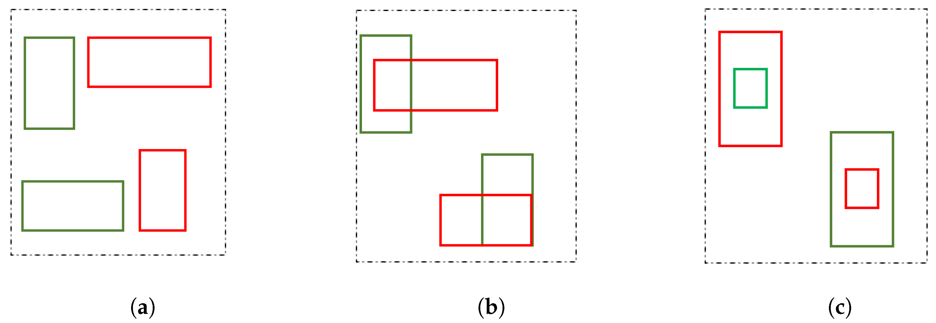
- Figure 3a represents cases of no overlap between predicted and ground truth boxes. In this scenario, the metric performed poorly because and → 0, the gradient also became 0, and → 1, a very high loss value. During these cases, network training is halted. This can be observed as a primary drawback.
- The secondary drawback was observed during partial and complete overlap of bounding boxes where the range was (0, 1). In Figure 3b, the overlap region remained the same even for prediction boxes of different sizes; in Figure 3c, a similar case can be observed, where the prediction box could be larger or smaller in size in comparison to the ground truth box. The metric does not regress on the basis of the aspect ratios and size of the bounding boxes. This leads to inaccurate predictions and errors in classification during dense object detections.
4.2. Generalised Intersection over Union (GIoU)
4.3. Distance Intersection over Union (DIoU)
4.4. Improved IoU Loss (IIoU)
| Algorithm 1 Improved intersection over union loss estimation. |
| Input: = , = . Output:
|
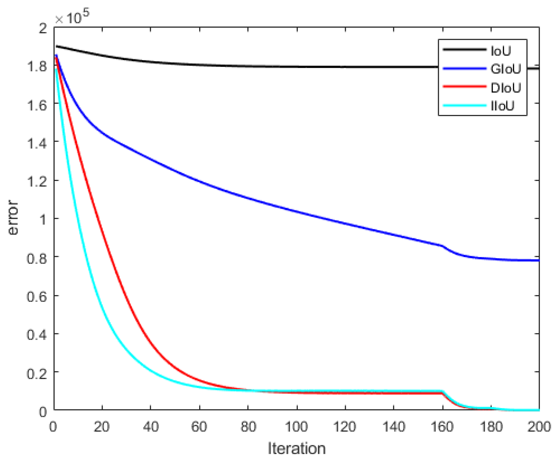
5. Simulation Experiment
| Algorithm 2 Simulation experiment on synthetic data. |
| Input: indicates anchor boxes at 115 scattered points within the central point at (10,10). S = covering 7 different scales and aspect ratio of the anchor boxes. is the set of ground truth boxes with centre (10,10) and 7 aspect ratios. corresponds to learning rate. Output: Regression error is calculated for each iteration and 115 scattered points.
|
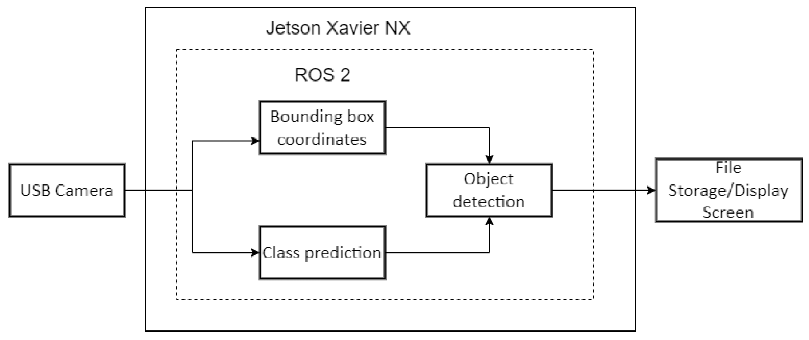
6. Embedded Deployment
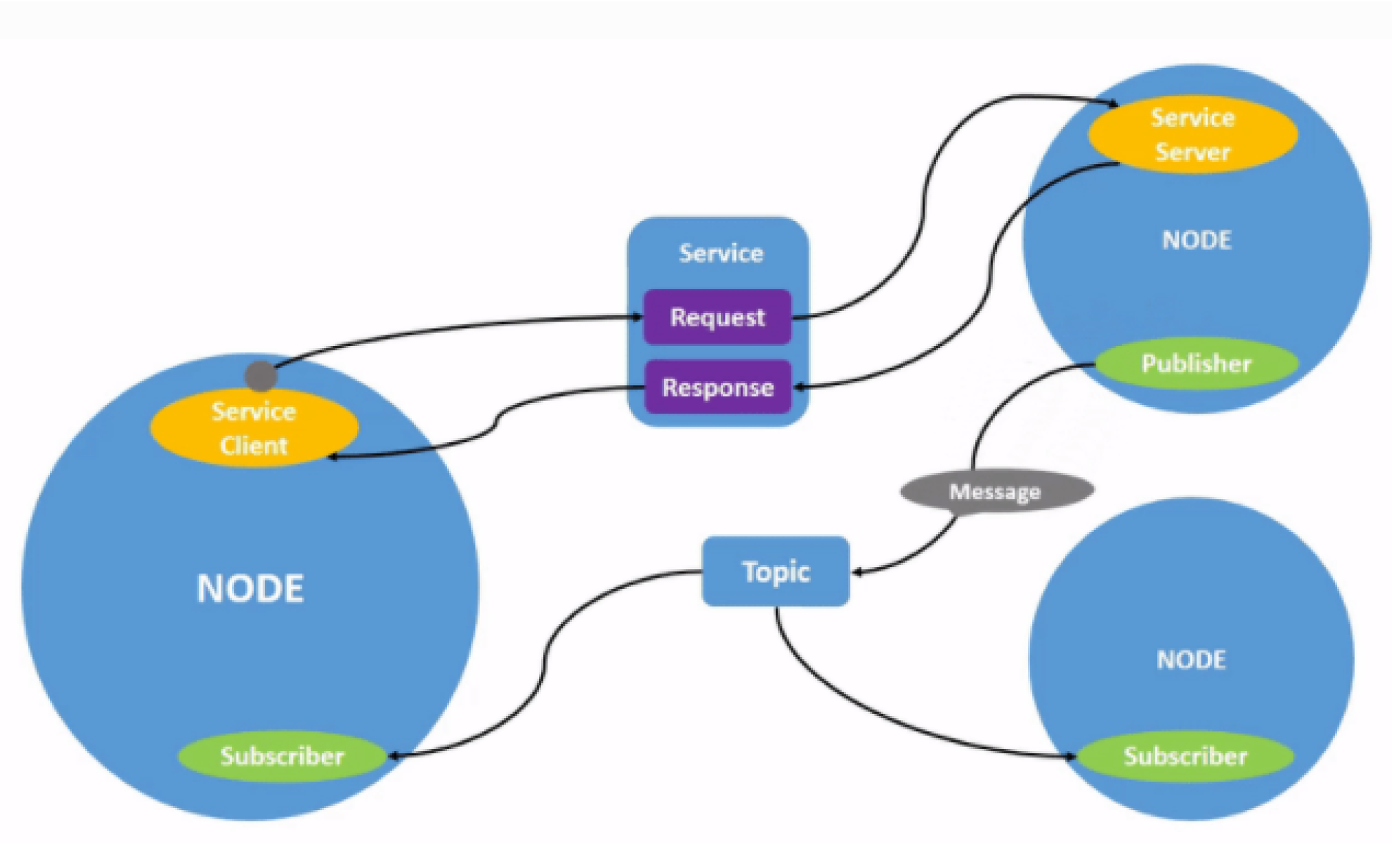
6.1. Robot Operating System(ROS)
6.1.1. ROS Filesystem Level
6.1.2. ROS Computation
6.1.3. ROS Community Level
6.2. Embedded System
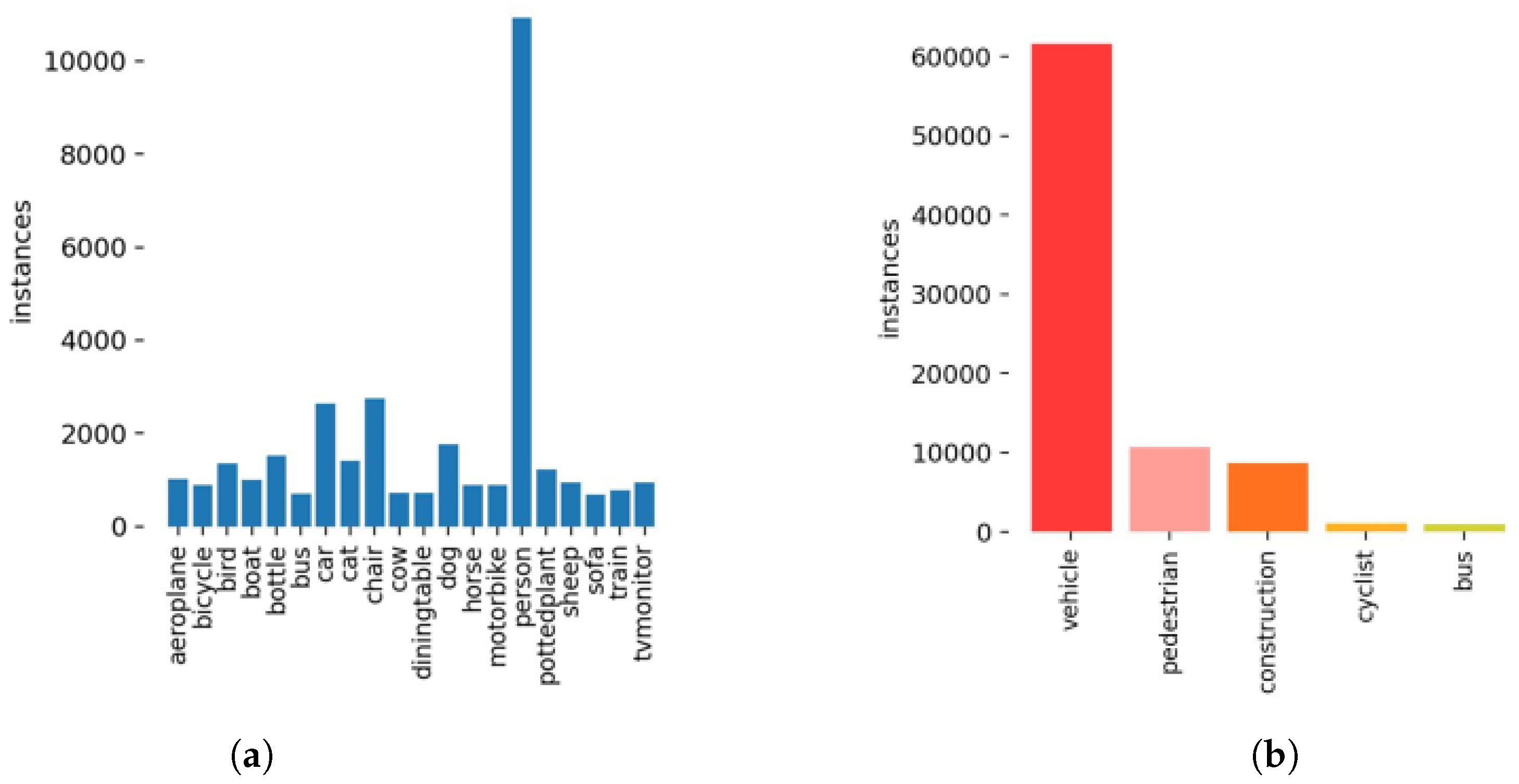
7. Dataset Preparation
8. Network Training and Testing Infrastructure
8.1. Training Infrastructure
- Intel Xeon Gold 6126 12-core CPUs;
- 12 GPU-accelerated Lenovo ThinkSystem SD530 deep learning;
- Tesla V100;
- Operating system: UBUNTU 18.04;
- Pytorch Version 1.7.1;
- Python 3.7.3.
8.2. Testing Infrastructure
- NVIDIA Jetson NX;
- ROS2 Foxy version;
- Logitech USB camera;
- Tesla V100;
- NVIDIA GeForce GTX 1080;
- Linux4tegra operating system (Ubuntu-derived OS);
- Pytorch Version 1.7.1;
- Python 3.7.3.
9. Performance Evaluation
9.1. Performance Evaluation on PASCAL and CGMU Datasets
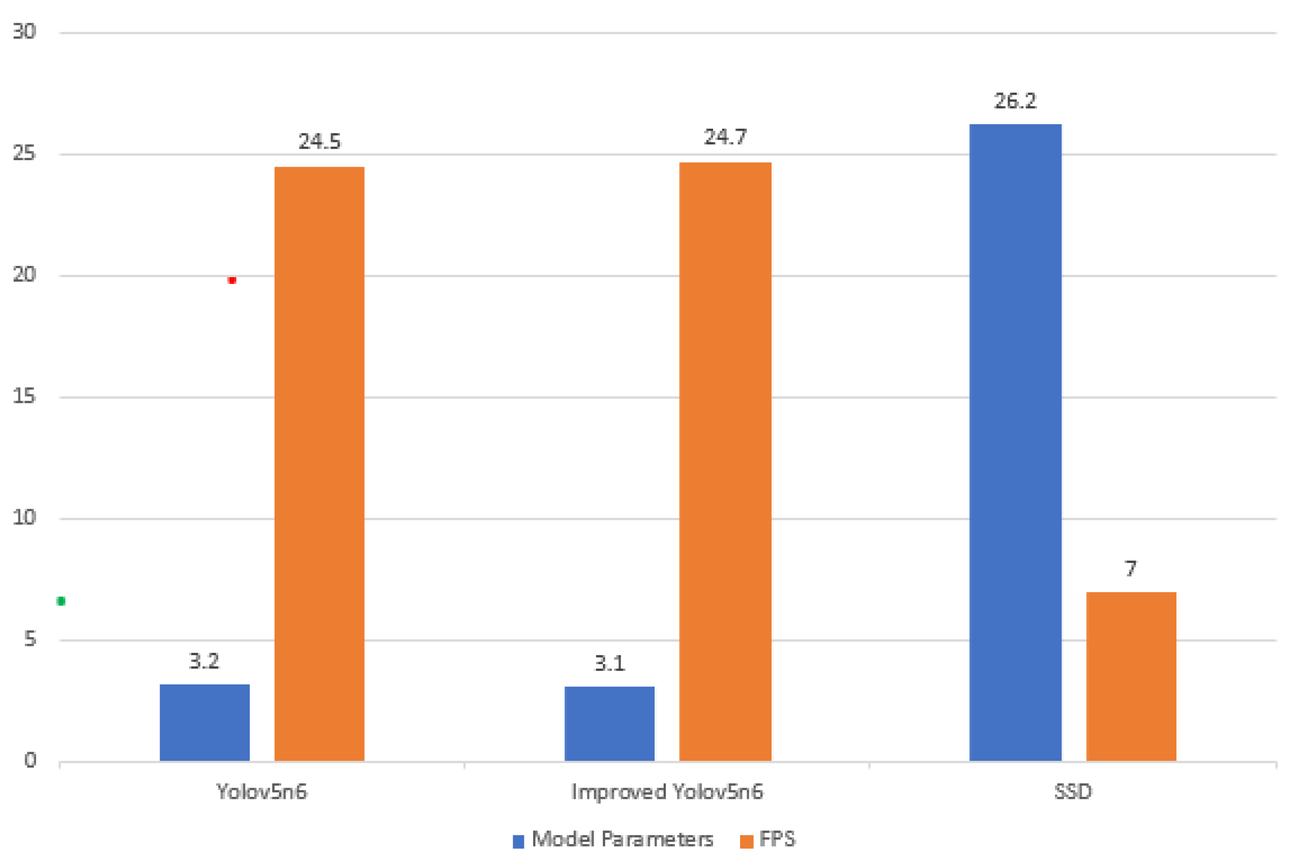
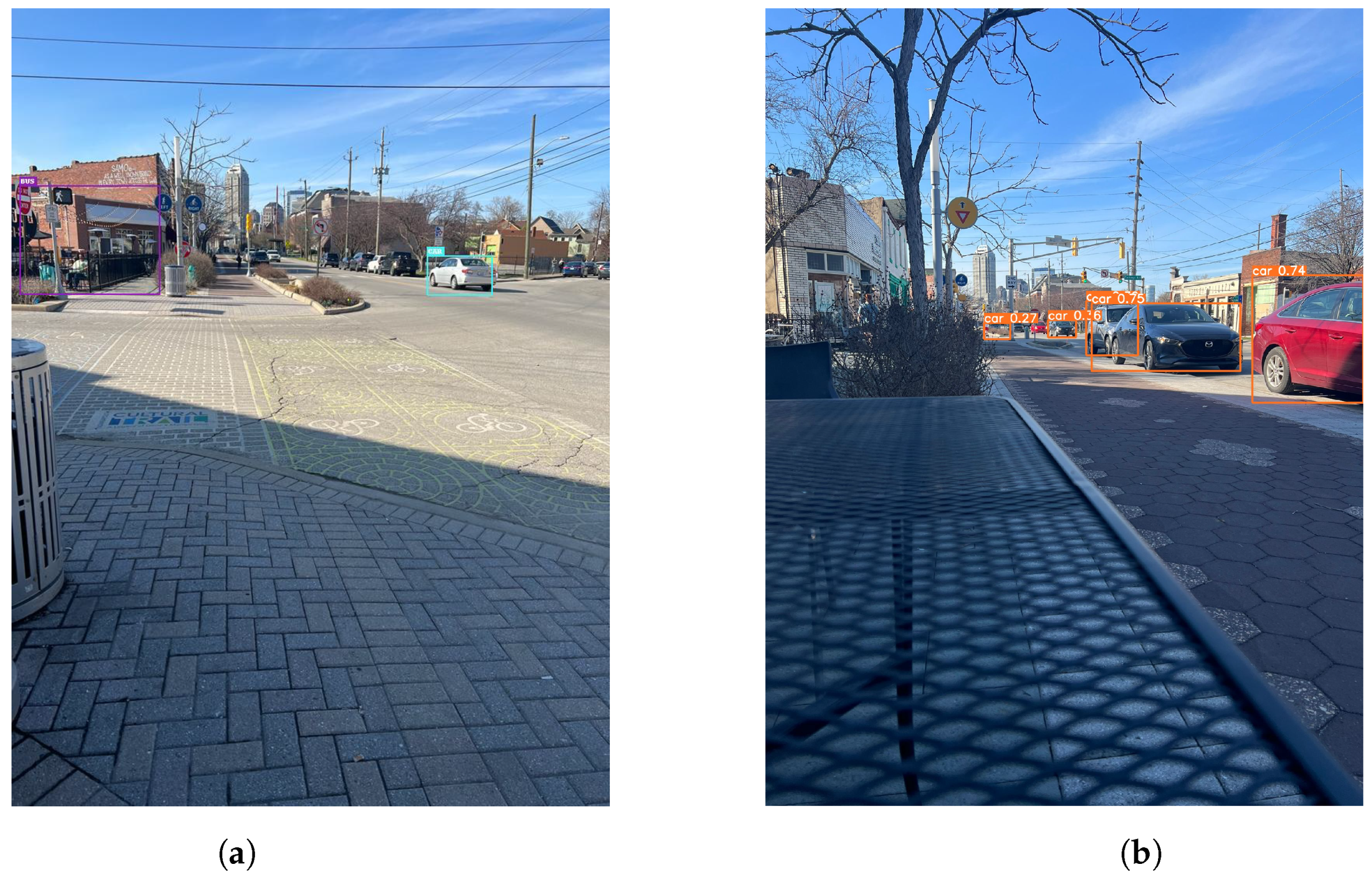
9.2. Real-Time Testing and Analysis
10. Conclusions
Author Contributions
Funding
Data Availability Statement
Conflicts of Interest
References
- Li, C.; Luo, Q.; Mao, G.; Sheng, M.; Li, J. Vehicle-mounted base station for connected and autonomous vehicles: Opportunities and challenges. IEEE Wirel. Commun. 2019, 26, 30–36. [Google Scholar] [CrossRef]
- Venkitachalam, S.; Manghat, S.K.; Gaikwad, A.S.; Ravi, N.; Bhamidi, S.B.S.; El-Sharkawy, M. Realtime Applications with RTMaps and Bluebox 2.0. In Proceedings of the on the International Conference on Artificial Intelligence (ICAI), Las Vegas, USA, 30 July–2 August 2018; pp. 137–140. [Google Scholar]
- Chitanvis, R.; Ravi, N.; Zantye, T.; El-Sharkawy, M. Collision avoidance and Drone surveillance using Thread protocol in V2V and V2I communications. In Proceedings of the 2019 IEEE National Aerospace and Electronics Conference (NAECON), Dayton, OH, USA, 15–19 July 2019; pp. 406–411. [Google Scholar] [CrossRef]
- Katare, D.; El-Sharkawy, M. Embedded System Enabled Vehicle Collision Detection: An ANN Classifier. In Proceedings of the 2019 IEEE 9th Annual Computing and Communication Workshop and Conference (CCWC), Las Vegas, NV, USA, 7–9 January 2019; pp. 0284–0289. [Google Scholar] [CrossRef]
- Girshick, R.; Donahue, J.; Darrell, T.; Malik, J. Rich feature hierarchies for accurate object detection and semantic segmentation. In Proceedings of the IEEE Conference on Computer Vision and Pattern Recognition, Columbus, OH, USA, 23–28 June 2014; pp. 580–587. [Google Scholar]
- Liu, W.; Anguelov, D.; Erhan, D.; Szegedy, C.; Reed, S.; Fu, C.Y.; Berg, A.C. Ssd: Single shot multibox detector. In European Conference on Computer Vision; Springer: Cham, Switzerland, 2016; pp. 21–37. [Google Scholar]
- Alex, K.; Sutskever, I.; Geoffrey, H. ImageNet classification with deep convolutional neural networks. Commun. ACM 2017, 60, 84–90. [Google Scholar]
- He, K.; Zhang, X.; Ren, S.; Sun, J. Deep residual learning for image recognition. In Proceedings of the 2016 IEEE Conference on Computer Vision and Pattern Recognition (CVPR), Las Vegas, NV, USA, 27–30 June 2016. [Google Scholar]
- Toma, A.; Wenner, J.; Lenssen, J.E.; Chen, J.-J. Adaptive Quality Optimization of Computer Vision Tasks in Resource-Constrained Devices using Edge Computing. In Proceedings of the 2019 19th IEEE/ACM International Symposium on Cluster, Cloud and Grid Computing (CCGRID), Larnaca, Cyprus, 14–17 May 2019. [Google Scholar]
- Tsimpourlas, F.; Papadopoulos, L.; Bartsokas, A.; Soudris, D. A design space exploration framework for convolutional neural networks implemented on edge devices. IEEE Trans. Comput. Des. Integr. Circuits Syst. 2018, 37, 2212–2221. [Google Scholar] [CrossRef]
- Ravi, N.; El-Sharkawy, M. Integration of UAVs with Real Time Operating Systems using UAVCAN. In Proceedings of the 2019 IEEE 10th Annual Ubiquitous Computing, Electronics & Mobile Communication Conference (UEMCON), New York, NY, USA, 10–12 October 2019. [Google Scholar]
- Borrego-Carazo, J.; Castells-Rufas, D.; Biempica, E.; Carrabina, J. Resource-Constrained Machine Learning for ADAS: A Systematic Review. IEEE Access 2020, 8, 4053–4059. [Google Scholar] [CrossRef]
- Katare, D.; El-Sharkawy, M. Real-Time 3-D Segmentation on An Autonomous Embedded System: Using Point Cloud and Camera. In Proceedings of the 2019 IEEE National Aerospace and Electronics Conference (NAECON), Dayton, OH, USA, 15–19 July 2019. [Google Scholar]
- Zou, Z.; Shi, Z.; Guo, Y.; Ye, J. Object detection in 20 years: A survey. arXiv 2019, arXiv:1905.05055. [Google Scholar]
- Redmon, J.; Divvala, S.; Girshick, R.; Farhadi, A. You Only Look Once: Unified, Real-Time Object Detection. In Proceedings of the 2016 IEEE Conference on Computer Vision and Pattern Recognition (CVPR), Las Vegas, NV, USA, 27–30 June 2016; pp. 779–788. [Google Scholar]
- Ieamsaard, J.; Charoensook, S.N.; Yammen, S. Deep Learning-based Face Mask Detection Using YoloV5. In Proceedings of the 2021 9th International Electrical Engineering Congress (iEECON), Pattaya, Thailand, 10–12 March 2021. [Google Scholar]
- Everingham, M.; Van Gool, L.; Williams, C.K.I.; Winn, J.; Zisserman, A. The Pascal Visual Object Classes (VOC) Challenge. Int. J. Comput. Vis. 2010, 88, 303–338. [Google Scholar] [CrossRef] [Green Version]
- CGMU Dataset. Available online: https://donnees.montreal.ca/ville-de-montreal/images-annotees-cameras-circulation#additional-info (accessed on 14 February 2022).
- Simonyan, K.; Zisserman, A. Very deep convolutional networks for large-scale image recognition. arXiv 2014, arXiv:1409.1556. [Google Scholar]
- Sam, S.M.; Kamardin, K.; Sjarif, N.N.A.; Mohamed, N. Offline Signature Verification using Deep Learning Convolutional Neural Network (CNN) Architectures GoogLeNet Inception-v1 and Inception-v3. Procedia Comput. Sci. 2019, 161, 475–483. [Google Scholar] [CrossRef]
- Deng, J.; Dong, W.; Socher, R.; Li, L.J.; Li, K.; Li, F.F. Imagenet: A Large-Scale Hierarchical Image Database. In Proceedings of the 2009 IEEE Conference on Computer Vision and Pattern Recognition, Miami, FL, USA, 20–25 June 2009; pp. 248–255. [Google Scholar]
- Zaidi, S.S.A.; Ansari, M.S.; Aslam, A.; Kanwal, N.; Asghar, M.; Lee, B. A survey of modern deep learning based object detection models. arXiv 2021, arXiv:2104.11892. [Google Scholar] [CrossRef]
- Zhao, Z.; Zhang, Z.; Xu, X.; Xu, Y.; Yan, H.; Zhang, L. A Lightweight Object Detection Network for Real-Time Detection of Driver Handheld Call on Embedded Devices. Comput. Intell. Neurosci. 2020, 2020, 6616584. [Google Scholar] [CrossRef] [PubMed]
- Redmon, J.; Farhadi, A. Yolov3: An incremental improvement. arXiv 2018, arXiv:1804.02767. [Google Scholar]
- Jadon, A.; Omama, M.; Varshney, A.; Ansari, M.S.; Sharma, R. FireNet: A specialized lightweight fire & smoke detection model for real-time IoT applications. arXiv 2019, arXiv:1905.11922. [Google Scholar]
- Rao, Y.; Yi, G.; Xue, J.; Pu, J.; Gou, J.; Wang, Q.; Wang, Q. Light-Net: Lightweight Object Detector. IEEE Access 2020, 8, 201700–201712. [Google Scholar] [CrossRef]
- Li, Y.; Li, J.; Lin, W.; Li, J. Tiny-DSOD: Lightweight object detection for resource-restricted usages. arXiv 2018, arXiv:1807.11013. [Google Scholar]
- Reed, R. Pruning algorithms-a survey. IEEE Trans. Neural Netw. 1993, 4, 740–747. [Google Scholar] [CrossRef]
- Han, S.; Mao, H.; Dally, W.J. Deep compression: Compressing deep neural networks with pruning, trained quantization and huffman coding. arXiv 2015, arXiv:1510.00149. [Google Scholar]
- Ren, S.; He, K.; Girshick, R.; Sun, J. Faster r-cnn: Towards real-time object detection with region proposal networks. Adv. Neural Inf. Process. Syst. 2015, 28, 1137–1149. [Google Scholar] [CrossRef] [Green Version]
- He, J.; Erfani, S.; Ma, X.; Bailey, J.; Chi, Y.; Hua, X.S. α-IoU: A Family of Power Intersection over Union Losses for Bounding Box Regression. Adv. Neural Inf. Process. Syst. 2021, 34. Available online: https://papers.nips.cc/paper/2021/hash/a8f15eda80c50adb0e71943adc8015cf-Abstract.html (accessed on 14 February 2022).
- Girshick, R. Fast r-cnn. In Proceedings of the IEEE International Conference on Computer Vision, Santiago, Chile, 7–13 December 2015. [Google Scholar]
- Uijlings, J.R.; Van De Sande, K.E.; Gevers, T.; Smeulders, A.W. Selective search for object recognition. Int. J. Comput. Vis. 2013, 104, 154–171. [Google Scholar] [CrossRef] [Green Version]
- Lin, T.Y.; Goyal, P.; Girshick, R.; He, K.; Dollár, P. Focal loss for dense object detection. In Proceedings of the IEEE International Conference on Computer Vision, Venice, Italy, 22–29 October 2017. [Google Scholar]
- Padilla, R.; Netto, S.L.; Da Silva, E.A. A survey on performance metrics for object-detection algorithms. In Proceedings of the 2020 International Conference on Systems, Signals and Image Processing (IWSSIP), Niteroi, Brazil, 1–3 July 2020. [Google Scholar]
- Hanley, J.A.; McNeil, B.J. The meaning and use of the area under a receiver operating characteristic (ROC) curve. Radiology 1982, 143, 29–36. [Google Scholar] [CrossRef] [Green Version]
- Kolawole, S.; Osakuade, O.; Saxena, N.; Olorisade, B.K. Sign-to-Speech Model for Sign Language Understanding: A Case Study of Nigerian Sign Language. arXiv 2021, arXiv:2111.00995. [Google Scholar]
- Zhu, L.; Geng, X.; Li, Z.; Liu, C. Improving YOLOv5 with Attention Mechanism for Detecting Boulders from Planetary Images. Remote Sens. 2021, 13, 3776. [Google Scholar] [CrossRef]
- Available online: https://github.com/ultralytics/yolov5 (accessed on 14 February 2022).
- Lin, T.Y.; Maire, M.; Belongie, S.; Hays, J.; Perona, P.; Ramanan, D.; Dollár, P.; Zitnick, C.L. Microsoft coco: Common objects in context. In European Conference on Computer Vision; Springer: Cham, Switzerland, 2014. [Google Scholar]
- Zhang, D.; Fan, S.S. Fault detection method of transmission line based on Yolo V3. Autom. Technol. Appl. 2019, 38, 125–129. [Google Scholar]
- Tang, J.; Liu, S.; Zheng, B.; Zhang, J.; Wang, B.; Yang, M. Smoking Behavior Detection Based On Improved YOLOv5s Algorithm. In Proceedings of the 2021 9th International Symposium on Next Generation Electronics (ISNE), Changsha, China, 9–11 July 2021. [Google Scholar]
- Yang, G.; Feng, W.; Jin, J.; Lei, Q.; Li, X.; Gui, G.; Wang, W. Face mask recognition system with YOLOV5 based on image recognition. In Proceedings of the 2020 IEEE 6th International Conference on Computer and Communications (ICCC), Chengdu, China, 11–14 December 2020. [Google Scholar]
- Yu, J.; Jiang, Y.; Wang, Z.; Cao, Z.; Huang, T. Unitbox: An advanced object detection network. In Proceedings of the 24th ACM International Conference on Multimedia, Amsterdam, The Netherlands, 15–19 October 2016. [Google Scholar]
- Rezatofighi, H.; Tsoi, N.; Gwak, J.; Sadeghian, A.; Reid, I.; Savarese, S. Generalized intersection over union: A metric and a loss for bounding box regression. In Proceedings of the IEEE/CVF Conference on Computer Vision and Pattern Recognition, Long Beach, CA, USA, 15–20 June 2019. [Google Scholar]
- Zheng, Z.; Wang, P.; Liu, W.; Li, J.; Ye, R.; Ren, D. Distance-IoU loss: Faster and better learning for bounding box regression. In Proceedings of the AAAI Conference on Artificial Intelligence, New York, NY, USA, 7–12 February 2020; Volume 34. [Google Scholar]
- Rivera, S.; Iannillo, A.K.; Lagraa, S.; Joly, C.; State, R. ROS-FM: Fast Monitoring for the Robotic Operating System (ROS). In Proceedings of the 2020 25th International Conference on Engineering of Complex Computer Systems (ICECCS), Singapore, 28–31 October 2020. [Google Scholar]
- Ciobanu, A.; Luca, M.; Barbu, T.; Drug, V.; Olteanu, A.; Vulpoi, R. Experimental Deep Learning Object Detection in Real-time Colonoscopies. In Proceedings of the 2021 International Conference on e-Health and Bioengineering (EHB), Iasi, Romania, 18–19 November 2021. [Google Scholar]
- Stewart, C.A.; Welch, V.; Plale, B.; Fox, G.; Pierce, M.; Sterling, T.; Indiana University Pervasive Technology Institute. IUScholarWorks. Available online: https://scholarworks.iu.edu/dspace/handle/2022/21675 (accessed on 14 February 2022).


| Loss Evaluation | AP50 | AP55 | AP60 | AP65 | AP70 | AP75 | AP80 | AP85 | AP90 | AP95 | AP |
|---|---|---|---|---|---|---|---|---|---|---|---|
| 78.6 | 76.1 | 73.2 | 69.2 | 64 | 57.5 | 48.5 | 36.4 | 20.1 | 2.8 | 52.7 | |
| 78.5 | 76.3 | 73.2 | 68.6 | 63.7 | 57 | 48.9 | 36.4 | 21.1 | 3.4 | 52.7 | |
| Relative improvement | −0.1 | 0.2 | 0 | 0.4 | −0.3 | 0.5 | 0.4 | 0 | 1 | 1.4 | 0 |
| 78.6 | 76.3 | 73.2 | 69.1 | 63.6 | 57.3 | 49.5 | 37.4 | 21.6 | 3.3 | 53 | |
| Relative improvement | 0 | 0.2 | 0 | −0.1 | −0.4 | −0.2 | 1 | 1 | 1.5 | 0.5 | 0.3 |
| 78.7 | 76.5 | 73.5 | 69.3 | 64.1 | 57.8 | 50.2 | 37.5 | 21.4 | 3.2 | 53.2 | |
| Relative improvement | 0.1 | 0.4 | 0.3 | 0.1 | 0.1 | 0.3 | 0.7 | 1.1 | 1.3 | 0.4 | 0.5 |
| Relative improvement% | 0.13 | 0.52 | 0.41 | 0.14 | 0.15 | 0.52 | 0.15 | 3.02 | 6.4 | 14 | 0.94 |
| Loss Evaluation | AP50 | AP55 | AP60 | AP65 | AP70 | AP75 | AP80 | AP85 | AP90 | AP95 | AP |
|---|---|---|---|---|---|---|---|---|---|---|---|
| 48.8 | 45.8 | 42.4 | 38.3 | 32.3 | 27.7 | 20.7 | 13.6 | 6.2 | 0.79 | 27.7 | |
| 49.6 | 46 | 42.9 | 38.6 | 34.2 | 28.5 | 22.1 | 14.7 | 5.6 | 1.0 | 28.3 | |
| Relative improvement | 0.8 | 0.2 | 0.5 | 0.3 | 1.9 | 0.8 | 1.4 | 1.1 | −0.6 | 0.21 | 0.6 |
| 49.5 | 46.5 | 43.1 | 39 | 33.2 | 28.3 | 22.2 | 13.2 | 6.4 | 1.2 | 28.3 | |
| Relative improvement | 0.7 | 0.7 | 0.7 | 0.7 | 0.9 | 0.6 | 1.5 | −0.4 | 0.2 | 0.41 | 0.6 |
| 52.1 | 48.6 | 44.6 | 40.5 | 35.5 | 28 | 18.5 | 11.6 | 4.6 | 0.6 | 28.5 | |
| Relative improvement | 3.3 | 2.8 | 2.2 | 2.2 | 3.2 | 0.3 | −2.2 | −2 | −1.6 | −0.19 | 0.8 |
| Relative improvement% | 6.76 | 11.6 | 5.18 | 5.74 | 9.9 | 0.11 | −10.6 | −14.7 | −25.8 | −24 | 2.89 |
Publisher’s Note: MDPI stays neutral with regard to jurisdictional claims in published maps and institutional affiliations. |
© 2022 by the authors. Licensee MDPI, Basel, Switzerland. This article is an open access article distributed under the terms and conditions of the Creative Commons Attribution (CC BY) license (https://creativecommons.org/licenses/by/4.0/).
Share and Cite
Ravi, N.; El-Sharkawy, M. Real-Time Embedded Implementation of Improved Object Detector for Resource-Constrained Devices. J. Low Power Electron. Appl. 2022, 12, 21. https://doi.org/10.3390/jlpea12020021
Ravi N, El-Sharkawy M. Real-Time Embedded Implementation of Improved Object Detector for Resource-Constrained Devices. Journal of Low Power Electronics and Applications. 2022; 12(2):21. https://doi.org/10.3390/jlpea12020021
Chicago/Turabian StyleRavi, Niranjan, and Mohamed El-Sharkawy. 2022. "Real-Time Embedded Implementation of Improved Object Detector for Resource-Constrained Devices" Journal of Low Power Electronics and Applications 12, no. 2: 21. https://doi.org/10.3390/jlpea12020021