1. Introduction
In this study, we investigate the integration of several additional efficient techniques that improve the solution methods for the lifelong multiagent pickup-and-delivery (MAPD) problem, which is an extended class of iterative multiagent pathfinding (MAPF) problems, to reduce the redundancy in concurrent task execution and the space usage of a warehouse map.
The MAPF problem is a fundamental problem in multiagent systems, and its goal is to find a set of shortest collision-free paths for multiple agents in a time-space graph. Two cases of agents colliding on a graph of a two-dimensional map must be avoided. A vertex collision is a situation where multiple agents simultaneously stay in the same vertex, and in an edge/swapping collision, two agents move from both ends of the same edge in opposite directions.
MAPF problems are motivated by various applications, including the navigation of mobile robots [
1], autonomous vehicles in warehouses [
2], a swarm of drones [
3], autonomous taxiing of airplanes [
4], autonomous car operation [
5], and video games [
6]. There are various studies of MAPF/MAPD problems and solution methods (
Table 1).
The solution methods for MAPF problems are categorized as either complete or incomplete methods. The former type finds an optimal solution under a criterion of optimization. The conflict-based search (CBS) algorithm [
7] is a complete solution method consisting of two levels of search processes. In a higher level, a tree-search method finds colliding situations of agents and inserts constraints that inhibit colliding moves by agents to the pathfinding problems at the lower level. Then each agent solves its pathfinding problem using the A* algorithm in a time-space graph under the inserted constraints. Since this class of solution methods requires relatively high computational cost, several efficient/approximate methods have been developed, including the priority-based search (PBS) [
8] and enhanced CBS (ECBS) [
9] algorithms.
The incomplete methods find quasi-optimal solutions in exchange for relatively low computational cost. There are several types of solution methods based on dedicated problem settings for them. In the cooperative A* (CA*) algorithm [
6], the A* algorithm [
10,
11] in a time-space graph is repeatedly performed for each agent with a predefined order of agents to find a collision-free path, where each path is reserved in such an order. This is a greedy approach where the agents simply avoid the previously reserved paths.
The priority inheritance with backtracking (PIBT) algorithm [
12,
13] repeatedly determines the moves of agents in each subsequent time step by reactively resolving collisions among agents. It employs a push-and-rotate operation and introduces the priority values of agents and a partial backtracking method.
The lifelong MAPD problem is an extended class of the iterative multiagent pathfinding problem [
12], where new travel paths of multiple agents are repeatedly planned at the ends of their travel. This problem models a system in automated warehouses with robot carrier agents, which are allocated to pickup-and-delivery tasks generated on demand.
Although there are various classes of optimization/routing problems related to logistics, including the variants of vehicle-routing problems [
14,
15], several dedicated solution methods are necessary for them. A unique setting of MAPF/MAPD problems is that they extend a traditional shortest pathfinding problem so that multiple (ideally) shortest paths for multiple agents must be found without collisions of agents in a time-space graph. Although several techniques for traveling-salesperson problems (TSPs) can be employed as a part of solution methods, the variants of MAPF problems generally focus on the lower layers of routing/pathfinding problems containing obstacles than that for TSPs.
A solution method for MAPD problems consists of task allocation to agents and an MAPF method for the allocated tasks. In the case of static problems with a fixed number of tasks, the task allocation problem is often formalized as a fundamental combinatorial problem [
16]. On the other hand, for lifelong MAPD problems, partially greedy task allocation methods are reasonable for tasks continuously generated on demand [
17].
While PIBT can also be effectively applied to several cases of lifelong MAPD problems, it cannot correctly work with a map containing dead ends.
The token passing (TP) algorithm [
17], which is a solution method for lifelong MAPD problems, is based on a greedy task allocation method and the CA* algorithm. With TP, each task is allocated to an agent in a specific order, and a travel path for the task is reserved. This class of algorithms solves well-formed MAPD problems, where the endpoints (EPs) of agents’ travel paths are considered to avoid deadlock situations on the paths. A well-formed problem has several types of EPs, including pickup, delivery, and parking locations, and the condition of the feasible solutions is defined with EPs. Then a solution method exclusively allocates each task to an agent under a rule to avoid conflicts among the endpoints of the agents’ paths.
Since there are redundancies in the problem settings themselves and the concurrency of the allocated tasks, several additional techniques have been proposed to reduce them in the solution methods. The multi-label A* (MLA*) algorithm [
18] improves the CA* algorithm by employing the knowledge of the agents’ pickup locations/times to prune and relax pathfinding for allocated tasks. The standby-based deadlock avoiding method (SBDA) [
19], which is a dedicated solution for maze-like maps with just a few EPs, dynamically places standby locations of agents for narrow maps.
However, opportunities undoubtedly exist for investigating the integration of additional efficient techniques with improvements for more practical solution methods. Such an investigation will also be a useful tool to consider several modes in agents’ moves. As an analysis and better understanding of the additional solution techniques based on endpoints, we incrementally integrate the techniques and experimentally investigate their contributions to the quality of task allocation and agents’ paths. We integrate several techniques: (1) prioritizing task allocation, (2) generalization of EP types, (3) relaxation of constraints excluding EPs from paths, (4) dummy retreat paths, and (5) the subgoal divisions of pickup-and-delivery tasks into TP. Our result reveals some significant complementary effects of integrated additional techniques and trade-offs among them in several cases of problem settings. In particular, the full combination of our selected techniques with several improvements, excluding an experimental version, resulted in the best makespan in most cases. We believe that our experimental analysis will contribute to further developments of efficient solution methods.
This work is an extension based on a conference paper [
20]. We refined its experimental results by adding new benchmark problems, improved our proposed methods including the subgoal division, and revised our paper’s description by adding detailed explanations and examples.
The rest of this paper is organized as follows. In the next section, we briefly describe related works. In
Section 3, we present the background of our study, including the multiagent pickup-and-delivery problem, a solution method called token passing, and additional efficient techniques that are integrated in our study. Then we describe our proposed approach in
Section 4. We complementarily integrate the additional techniques with several improvements and apply our solution methods to an environment with relatively narrower maps. We experimentally investigate our approach in
Section 5, discuss several issues in
Section 6, and conclude in
Section 7.
Table 1.
MAPF/MAPD problem and approaches.
Table 1.
MAPF/MAPD problem and approaches.
| MAPF |
|---|
| Approach | Solver | Technique | Variants | Note |
|---|
| Offline MAPF |
| Exact | CBS [7] | Tree search to resolve collisions A* in time-space | ECBS [9], PBS [8] | Relatively high computational cost |
| Greedy/ Heuristic | CA* [6] | Greedy ordering of agents A* in time-space | | |
| Iterative MAPF |
| Greedy/Heuristic | PIBT [12] | Priority of agentsPush-and-rotate/backtracking | winPIBT [13] | Graphs (maps) with cycles |
| MAPD |
| Approach | Solver | Task allocation | MAPF | Note |
| Offline MAPD |
| Heuristic | TA-Prioritized/ TA-Hybrid [16] | TSP | Heuristic/ max-flow | |
| Lifelong MAPD |
| Greedy/Heuristic | TP [17] | Greedy | Variant of CA* | Well-formed
problems |
| MLA* [18] |
| PIBT (for MAPD) | PIBT | Graphs (maps) with cycles |
| SBDA [19] | Variant of CA* | Maze-like maps |
2. Related Works
In this section, we describe related works by extending our explanation from the previous section. We start with the multiagent path finding (MAPF) problem and briefly describe the extended classes of problems including iterative MAPF ones. Then we discuss multiagent pickup-and-delivery (MAPD) problems which are another iterative MAPF problem. For the classes of problems we refer to several solution methods. Finally we focus on a solution method for a class of MAPD problems and several additional techniques to improve such methods. Since the relationship among the classes of problems and the solution methods is slightly complicated, we summarize most of them in
Table 1 in advance.
The MAPF problem is a base of the MAPD problem, and solution methods for MAPF problems are also employed for MAPD problems. The solution methods of MAPF problems are categorized as either complete or incomplete methods. The complete solution methods find optimal solutions without collisions in the agents’ paths under a criterion of optimality. Typical criteria are the total number of moves for all agents and the makespan, which is the time required to complete the moves of all the agents.
The conflict-based search (CBS) [
7] is a complete solution method that employs two levels of search processes. In the higher level, a tree-search method finds the conflicts of the agents’ paths and resolves them by inserting constraints. On the other hand, in the lower level, a pathfinding method in a time-space graph is performed under the inserted constraints. Here each agent initially has its own shortest path ignoring other agents. The colliding situations between two agents are incrementally identified and inhibited in a tree search so that each agent recomputes its path avoiding such collisions. Since this method requires relatively high computational cost, efficient/approximate methods have been proposed [
8,
9]. In several studies, a MAPF problem was formalized as a satisfiability, satisfiability modulo theories, or answer set programming problem, and a dedicated solver for such a problem was employed [
21,
22,
23].
There are solvable and unsolvable MAPF problems. Intuitively, if a map has no sufficient space, agents cannot avoid each other [
17]. This situation also depends on the population density of the agents.
The incomplete solution methods do not assure the optimality of solutions, and they generally need relatively low computational cost. Such methods usually depend on specific feasible problem settings.
The cooperative A* (CA*) algorithm [
6] finds and reserves each agent’s travel path in a predefined order of agents. The collision avoidance in this approach basically depends on consistent reservations of agents’ travel paths. During the pathfinding, the A* algorithm is performed in a time-space graph under the previously reserved agents’ paths.
A different approach employs the push, rotate, and swap operations to resolve collisions among agents’ moves [
24,
25]. Here the agents have their default shortest paths ignoring other agents and basically resolve their collisions on demand. This partially resembles sliding puzzles or Sokoban. The priority inheritance with backtracking method (PIBT) [
12,
13] based on push-and-rotate operations manages the priority values of agents and employs a limited backtracking method in the push operation. Although the solution method is designed for a specific type of problem where all the vertices in a map’s graph are contained in cycles, it effectively resolves collisions among agents.
There are several extended classes of MAPF problems. An important example is the iterative MAPF problem [
12], where each agent updates its new goal location at its current goal. Other extended problem settings addressed various more practical situations, including delays in agents’ moves [
26,
27], continuous time in the moves [
28,
29], the asynchronous execution of tasks [
30], moves to any direction [
31], and agents with a specific type of bodies [
32]. Dedicated solution methods were also developed for the extended problems.
The multiagent pickup-and-delivery (MAPD) problem is a class of iterative MAPF problems where agents are allocated to transportation tasks, and the lifelong MAPD problem addresses tasks generated on demand [
17]. The lifelong MAPD problem is a class of iterative MAPF problems, since each agent has its sequence of goal locations for pickup-and-delivery tasks that are sequentially allocated to the agent. A single pickup-and-delivery task itself of a MAPD problem can also be considered an iterative MAPF problem because it has a subgoal of a pickup location.
Several solution methods for iterative MAPF problems and MAPD problems basically perform iterative processes for a sequence of (sub-)goals. However, the details of the solution processes are various.
The typical criteria of optimality in lifelong MAPD problems are the service time to complete each task and the makespan. A solution method for MAPD problems is decomposed into task allocation to agents and the MAPF for agents with allocated tasks. For a static problem with a fixed number of tasks, task allocation can be solved with a complete search method, although the issue of computational complexity remains. Task allocation can be represented as several types of combinatorial optimization problems, including the traveling-salesperson problem (TSP) [
16].
We note that TSP is employed not to solve the routing of agents but to sort their allocated tasks as a cycle graph. Although perhaps MAPF/MAPD problems can be integrated with several vehicle-routing problems (VRPs) [
14,
15], a relatively large gap appears to exist between them in both the problem definitions and the solution methods. For these classes of methods, several solution methods for TSPs and VRPs are employed, including local search methods [
33], genetic algorithms [
34], and machine learning approaches [
35,
36,
37]. Extended classes with multiple agents contains combinatorial problems of agents and routes, and dedicated extended solution methods are employed [
37,
38]. On the other hand, MAPF/MAPD problems are extensions of a traditional shortest pathfinding problem and generally focus on the lower layers of routing/pathfinding problems containing obstacles and other colliding agents. Several demand-responsive transport (DRT) systems [
39] also employ multiple vehicles, while their collisions are generally excluded from problem settings. Here a transport simulation itself is also a major interest.
When tasks are generated on demand, task allocation is solved using (partially) greedy approaches. In addition, greedy approaches for iterative MAPF problems are often reasonable for the scalability of solution methods.
The token passing (TP) algorithm [
17] is a solution method for lifelong MAPD problems. It employs a greedy task allocation method and the CA* algorithm. This solution method depends on the condition of well-formed problems [
17,
40] and employs a set of rules considering the endpoints of agents’ travel paths in the task allocation to avoid deadlock situations among agents. While PIBT can also be employed for MAPD problems, the conditions of feasible problems are different from that of TP. In particular, PIBT cannot be applied to maps containing dead ends.
Since a solution method based on well-formed problems suffers some redundancy in the parallel execution of tasks, several methods, including additional efficient techniques (
Table 2), have been proposed to reduce the redundancy.
The multi-label A* (MLA*) algorithm [
18], which has been used instead of the CA* algorithm, considers agents’ pickup locations/times in the pathfinding to prune the search and relax the restriction of paths. This previous method also employs an ordering of agents in the task allocation that is based on the minimum heuristic path length from the location of a currently available agent to the pickup location of each new task. However, it determines whether the allocation of each task to an agent is possible by executing the MLA* algorithm. On the other hand, the effect of the MLA* algorithm resembles that of another method employed in our study. Moreover, our selected method considers the estimated pickup time of each new task for all the agents, including currently working agents, and do not require a pathfinding process to verify whether the allocation of each task is possible.
Several methods that improve TP partially relax the conditions of the well-formed problems that ensure feasible solutions. The standby-based deadlock avoiding method (SBDA) [
19] is a relatively aggressive approach that employs dynamically prepared standby locations of agents. However, it mainly addresses a special case of maze-like maps with a small number of parking, pickup, and delivery locations. We address the case of warehouse maps that generally contains a sufficient number of such locations.
In this study, we focus on additional techniques to improve the performance of TP. While there are several existing works on such components, opportunities must be found to investigate the effect of integrating such additional techniques to analyze the redundancy in the solution process that can be reduced by the integrated techniques.
We employ several additional techniques with the TP algorithm to mainly improve the concurrency of tasks and the space usage of warehouse maps. To investigate integrated solution methods based on additional techniques, we carefully selected a set of fundamental ones that have different and complementary effects (
Table 2) and incrementally combine them.
Table 3 shows the possible full combinations of them in our result.
3. Background
In this section, we present the background of our study. We first introduce the MAPD problem and the TP algorithm. Then we describe our selected additional techniques (partially listed in
Table 2) for improving the TP algorithm as the basis of our integrated solution methods.
3.1. Lifelong Multiagent Pickup-and-Delivery Problems
The lifelong multiagent pickup-and-delivery (MAPD) problem [
17] is an extended class of multiagent pickup-and-delivery problems and iterative multiagent pathfinding (MAPF) problems. Here multiple pickup-and-delivery tasks are generated on demand during a certain period and repeatedly allocated to agents. For these allocated tasks, collision-free travel paths of agents are determined. A problem consists of the following:
undirected graph representing a warehouse’s map,
a set of agents , and
a set of currently generated pickup-and-delivery tasks .
Each task has the information of its pickup-and-delivery locations , where . An agent assigned to a task travels from its current location to the pickup location and then to the delivery location.
Let denote the location of agent in discrete time step t. Agent moves from to an adjacent location or stays in its current location at the end of each time step t. An agents’ path is the sequence of its moves for a period of time steps.
There are two cases of colliding agents’ moves to be avoided. First, two agents and collide if they simultaneously stay in the same location (vertex conflict): . Second, the agents collide if they simultaneously move on the same edge from both ends of the edge (edge/swapping conflict): . The paths of two agents collide if there are at least one colliding move on them.
The condition of a well-formed MAPD problem that guarantees feasible solutions without deadlock situations in task allocation and multiple pathfinding has been presented [
17,
40]. Here the vertices, which can be the first and last positions of each path, are called endpoints (EPs). In the case of lifelong MAPD problems, an EP can be pickup, delivery, and parking locations.
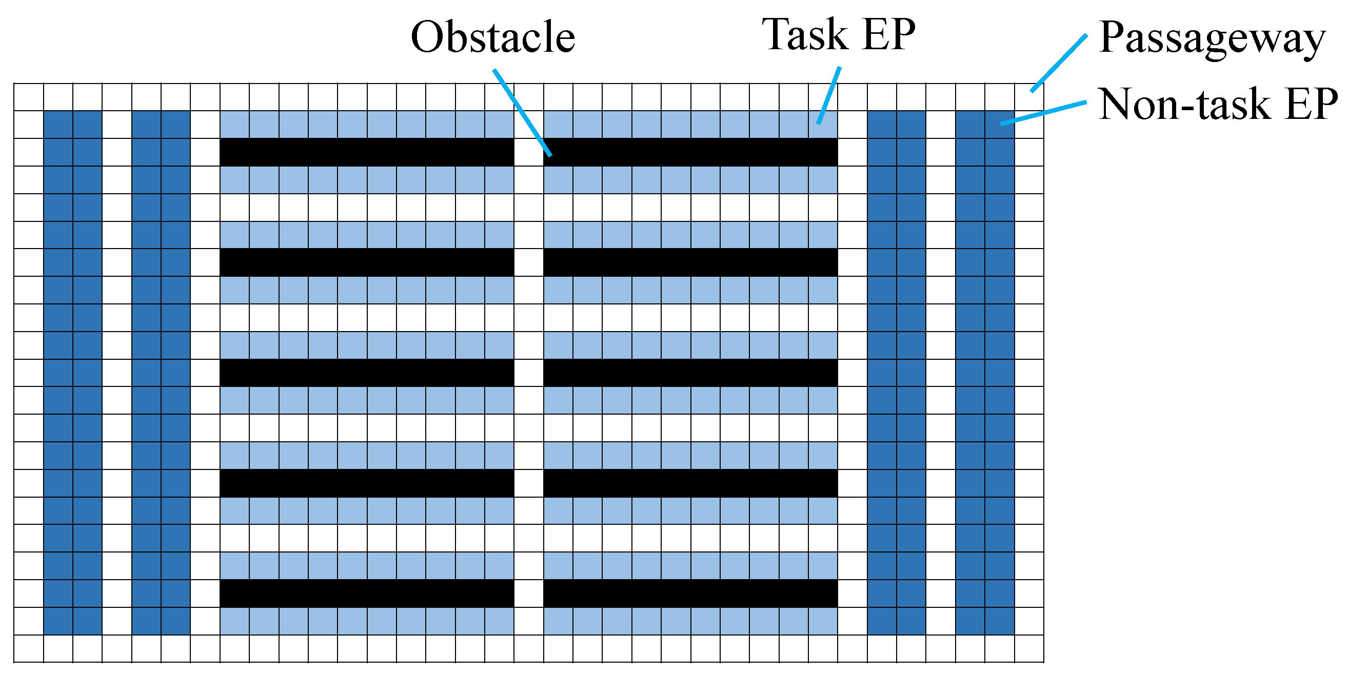
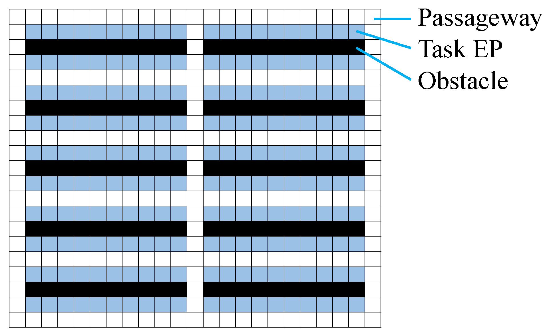
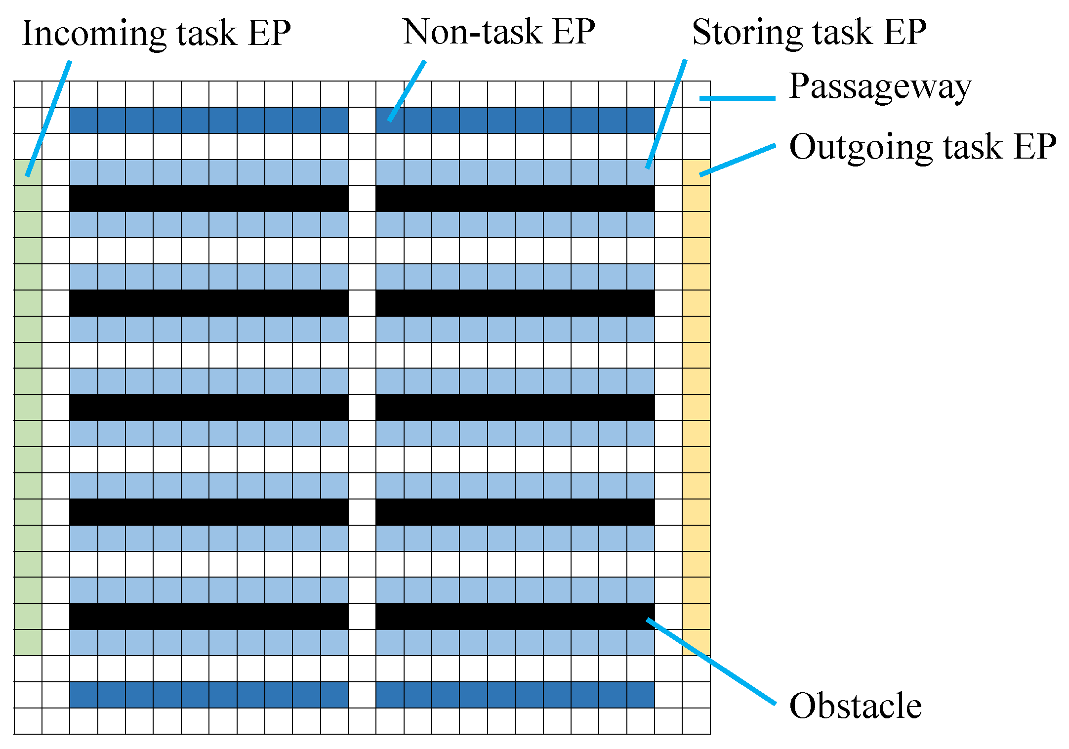
In a fundamental well-formed problem, EPs
are categorized into non-task EPs
, which are initial and parking locations, and task EPs
, which are pickup-and-delivery locations (
Figure 1). Here
. With these EPs, the conditions for a well-formed problem are defined as follows (Definition 1 in [
17]).
A MAPD is well-formed iff
the number of tasks is finite,
non-task endpoints are no fewer than the number of agents, and
for any two endpoints, there exists a path between them that traverses no other endpoints.
Under the following rules, tasks can be sequentially allocated to agents without deadlock situations among the paths for the allocated tasks.
Each path of an agent only contains EPs for the first and last locations of the agent (and a pickup location), and
the last location of each path is not included in any other paths.
The maps of warehouses are generally represented using grids in fundamental studies, and we interchangeably use a vertex in a graph, a cell in a grid world, and a location in a map.
3.2. Solution Method Based on Endpoints
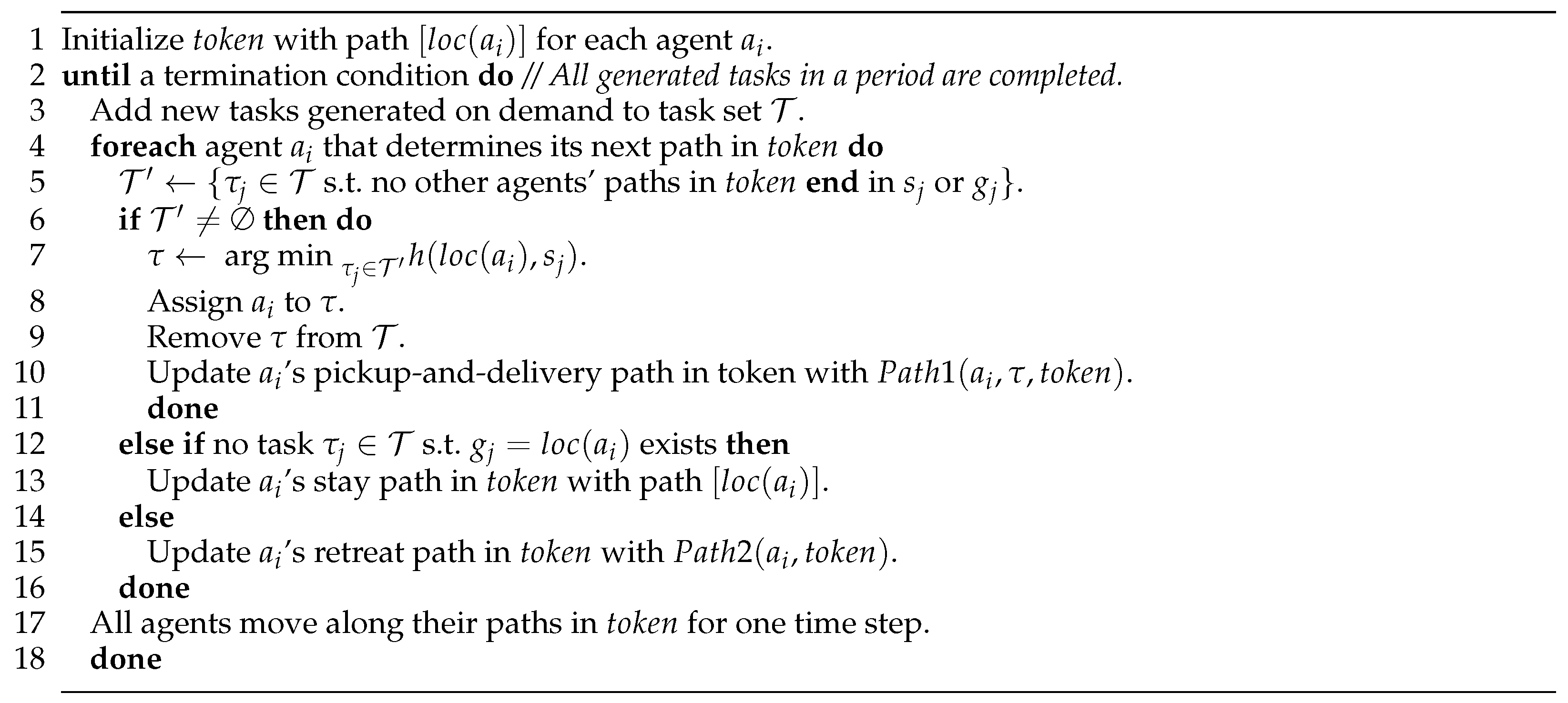
The token passing (TP) algorithm [
17] is a fundamental method to solve well-formed MAPD problems (
Figure 2). Here a cooperative system is assumed to consists of multiple agents and a centralized process that adds new tasks.
In the pseudo code in
Figure 2, we employ the following notations:
: agent a’s location;
and : pickup-and-delivery locations of task ;
: heuristic distance from v to ;
and : pathfinding and reservation methods for a pickup-and-delivery path of task and a retreat path.
The agents sequentially allocate their tasks and reserve corresponding travel paths in a greedy order (line 4) by referring and updating a shared memory called a token (lines 1, 4–5, 10, 13, 15, and 17 in
Figure 2). A token contains the information of a list of tasks waiting to be allocated and the paths reserved by the agents.
Each agent without an assigned task tries to allocate a new task that do not cause a deadlock situation under the currently reserved paths. If such a task is allocated, the agent finds and reserves a path that corresponds to its assigned task by the A* algorithm on a time-space graph (lines 6–11).
Here the tasks are prioritized by the distance from the agent’s current location to the pickup location for each task (line 7).
For heuristic function , we employ the distance in a two-dimensional map with fixed obstacles (shelves) and without agents. The distance value can be cached for the end of the current travel path of each agent and each endpoint, and a cached distance value is updated when a corresponding agent’s reservation is updated.
If any waiting tasks cannot be assigned to an agent, the agent remains at its current EP or retreats to one of other EPs. If its current location is the delivery location of a task on the task list, the agent retreats to a free EP that does not conflict with the delivery locations of the tasks on the task list and the reserved paths (line 15).
Otherwise, the agent temporarily stays at its current location (line 13). The agent also reserves a retreat or a stay path (lines 10, 13, and 15). At the end of each time step, each agent moves or stays, as it reserved (line 17).
There is some redundancy in this basic solution method, and several techniques below have been proposed to address this problem.
3.3. Prioritizing Task Allocation Considering Estimated Pickup Times
The task allocation process can employ several ordering criteria to select a waiting task to be assigned to a free agent. Although there are many possible heuristic criteria, there might be some trade-offs among them in different problem instances [
18]. Here we focus on a heuristic based on the estimated pickup time of tasks [
41] as a reasonable example.
Since TP is based on the reservation of paths, the time of the last location on each reserved path is known. Therefore, to estimate agent ’s pickup time of task , the heuristic distance from the agent’s current goal location to the task’s pickup location is added to the (future) time at the agent’s goal location: .
Each agent , which selects its new task to be allocated, compares the estimated pickup time of each task with that of other agents. If the estimated pickup time of one of the other agents is earlier than that of the selecting agent, the allocation of the task is postponed.
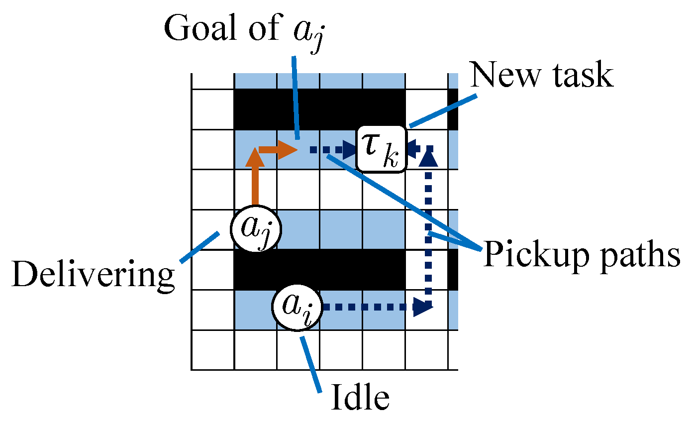
In the example shown in
Figure 3, idle agent
without a task can pick up new task
in eight time steps, while delivering agent
can pick it up in five time steps including its current delivery time. Therefore, agent
does not immediately select
and tries to select the nearest task among other new ones.
3.4. Relaxation of Paths Containing Arbitrary EPs
To reduce the redundancy in path lengths, an additional technique was proposed, where paths are allowed through EPs [
41]. While paths can contain any EPs in this extension, the deadlock situations of paths are avoided by considering conflicting EPs in task allocation.
Here all the EPs in all the reserved paths are locked, and the conflict between the locked EPs and the delivery location of each new task in the task list is checked. Each agent also temporarily reserves its additional ’staying’ path at the end of its current path until it cancels the staying reservation and reserves a new path. This information is referred to in the pathfinding for a newly assigned task to avoid the locations at which agents are staying. The effect of this technique partially resembles the pruning and relaxation in pathfinding improved by the MLA* [
18] algorithm. With this technique, the length of travel paths can be reduced, although such paths might block more EPs and decrease the number of allocatable tasks.
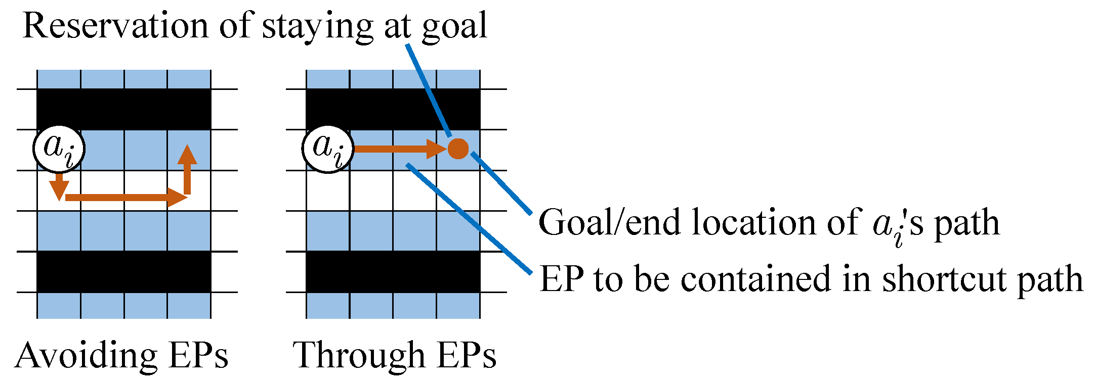
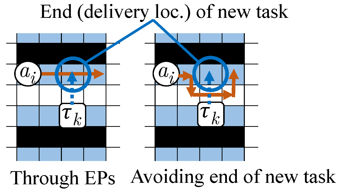
Figure 4 shows an example where the length of
’s travel path can be reduced by moving through EPs. In this example, in both the left and right side cases, agent
’s path ends at the third cell to the right from
’s current (start) location. While the EPs between the start and end locations of
cannot be shortcuts in the original TP algorithm (left side case), the extended method allows a shortcut through EPs (right side case). Agent
temporarily reserves a continuous stay at its goal location in addition to its reserved path. The reservation at the current goal location is canceled when a new task is allocated to the agent.
3.5. Adding Dummy Path for Retreating
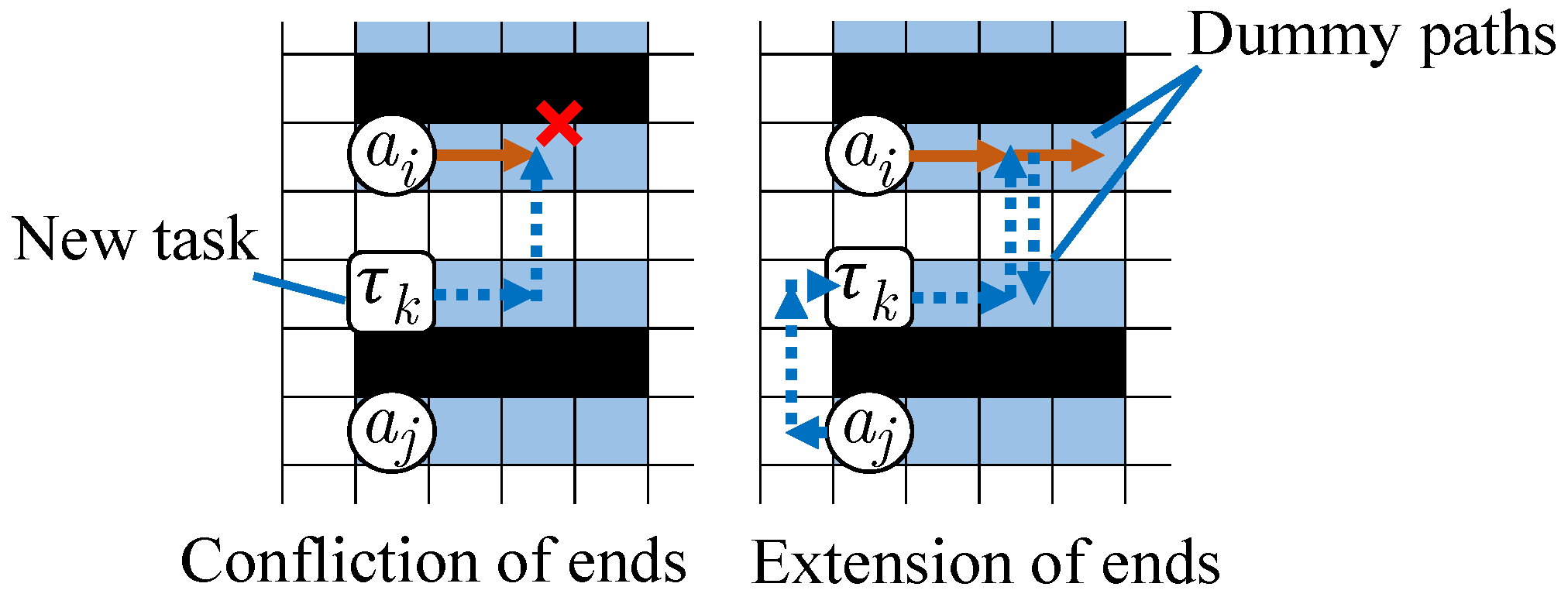
The task allocation is affected by the locked task endpoints that are the last locations of the reserved paths. If a task’s delivery location is locked, such a task cannot be assigned to avoid deadlock situations of paths. To reduce the number of locked tasks, additional dummy paths are introduced [
16,
42]. By adding a dummy path, an agent’s path is expanded so that it retreats to a non-task endpoint with no waiting tasks.
A dummy path is created with the destination of a free non-task EP that is not locked by other agents’ paths so that an agent reduces the situations where the delivery locations of waiting tasks are locked at the end of the agent’s path. An agent selects the destination of its new dummy path from free non-task EPs by referring to the task list and the reserved paths of other agents. Note that the ends of a path in the TP algorithm must be EPs. Therefore, the destination of an additional dummy path is always a free EP (a non-task EP in the previous study).
In addition, such a dummy path might be canceled, if necessary. The additional staying path of an agent shown in
Section 3.4 is a special case of a dummy path. Dummy paths can reduce the number of locked tasks, while the agents might reserve relatively long retreat paths if non-task endpoints are located in separate areas in a warehouse.
In the example in
Figure 5, the goal locations of agent
and new task
were originally identical, and
cannot be allocated to any agents. By adding dummy paths from their common goal location to two different EPs, such a conflict is resolved, and task
can be allocated to an agent.
In a basic case, each dummy path starts from the last location of a path and ends at a parking location [
16].
3.6. Partial Reservation of Tasks’ Paths
In lifelong MAPD problems, tasks generated on demand are continuously allocated to multiple agents depending on the situation in each time step. Such a situation might change before an agent traverses a long path, and this can affect the allocation of new tasks and paths.
For this issue, several methods divide the paths of tasks to delay the planning of future paths [
13,
42]. While there are several relatively complex methods to employ such a partial path within a time window, we focus on a relatively simple method that divides the path of a single task into pickup and delivery paths.
4. Integration and Improvement of Efficient Techniques
To investigate the effects and trade-offs of integrated solution methods based on the additional techniques shown in the previous section, we improve some details of the techniques and incrementally combine them. We also address problems without non-task endpoints.
Our selected additional approaches that have different and complementary effects are summarized in
Table 2. In the following, we incrementally combine these techniques. Possible full combinations of them in our result are shown in
Table 3.
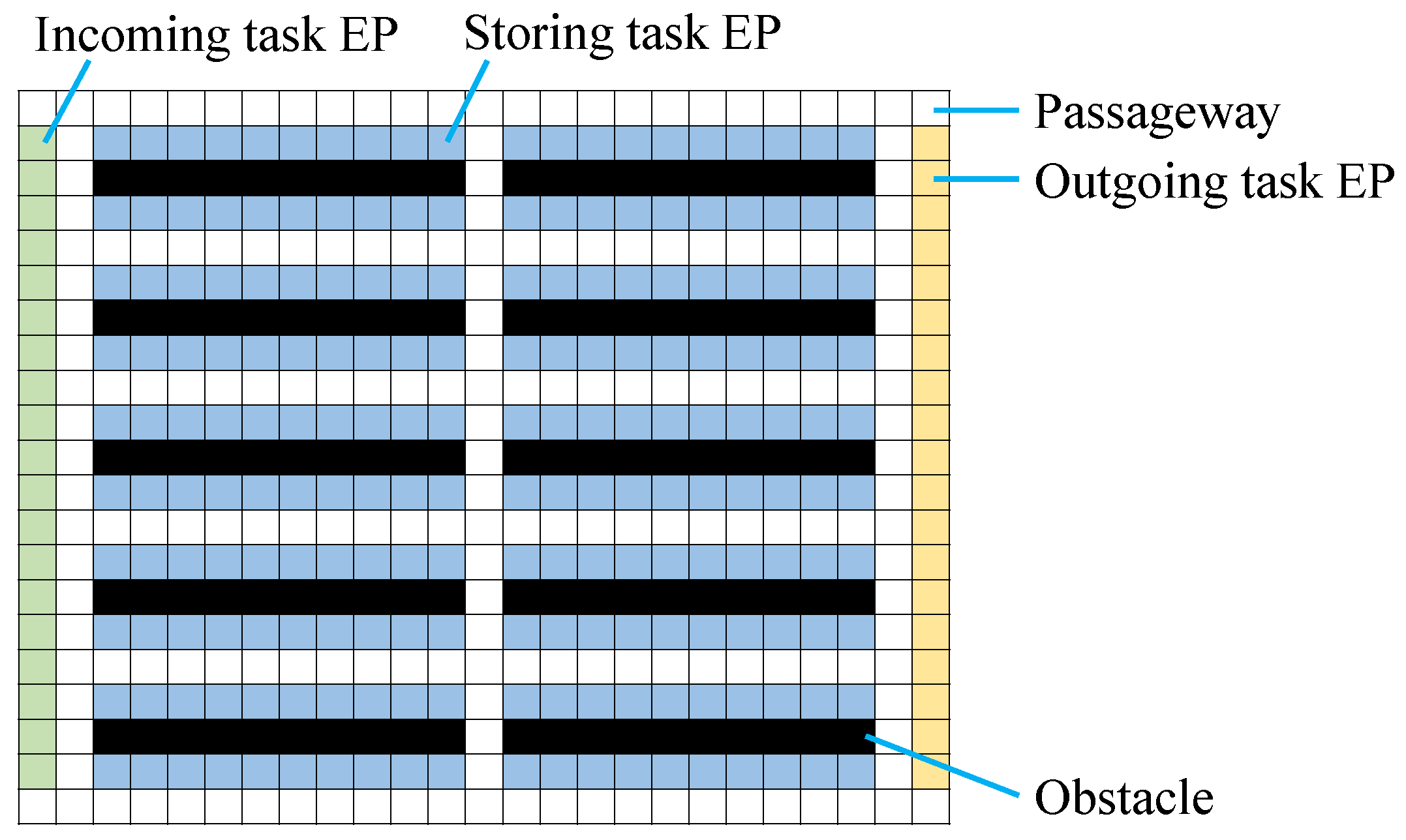
4.1. Generalization of Task and Non-Task EPs
To reduce the redundant space in warehouses, we allow cases where the initial and retreat locations of agents can be any EPs, including maps without non-task EPs (
Figure 6). In this example, the left and right side areas with non-task EPs in the map in
Figure 1 are eliminated. This case requires the relaxation of the second condition for well-formed MAPD problems in
Section 3.1 that non-task endpoints must not be fewer than the number of agents. Instead, the space usage of warehouses is reduced. In the modified settings, each agent basically retreats to its nearest EP, excluding EPs on the reserved paths and those of the delivery locations of tasks waiting to be allocated. When no EP temporarily exists to retreat to in an environment with fewer non-task EPs than agents, such an agent stays at its current EP.
Even in this modified setting, all tasks can be completed without any deadlock situations for a finite number of on-demand tasks. In specially limited cases without non-task EPs, there are solutions as long as the number of agents is less than the number of task EPs .
Proposition 1. The relaxed well-formed problem without non-task EPs can be solved with a modified TP algorithm, if the number of agents is less than the number of task EPs.
Proof of Proposition 1. We briefly sketch this proof. In the TP algorithm, tasks are sequentially allocated to agents under previously allocated tasks and reserved paths. The reservation of the stay/retreat paths of agents is also performed in the same procedure. Therefore, the movements of agents are serialized in the worst case without deadlock situations as long as at least an agent’s new path can be reserved.
If there is only a single free EP , one agent can move to it. A new task whose delivery location is can be allocated to an idle agent. Otherwise, can be the goal location of another agent that retreats from a delivery location of new tasks. Such retreat moves of agents might be repeated until a new task is allocated.
Agent at a pickup location of a waiting task can immediately allocate the task to after an agent in the task’s delivery location reserves a retreat path. In addition, in our modified method, agents do not retreat to EPs on reserved paths or to the delivery locations of new tasks waiting to be allocated.
Therefore, at least a single task can be sequentially performed if the number of agents is less than the number of EPs. □
The map in
Figure 6 contains 200 (task) EPs, and at most 199 agents can be deployed. On the other hand, the map in
Figure 1 contains 152 non-task EPs, and only the same number of agents can be deployed under the conditions for well-formed MAPDs.
4.2. Employing Task Allocation Considering Estimated Pickup Times
We first integrate the generalization of EPs shown in the previous subsection and the task allocation considering the estimated pickup times (
Section 3.3). While we borrowed the idea from a previous study [
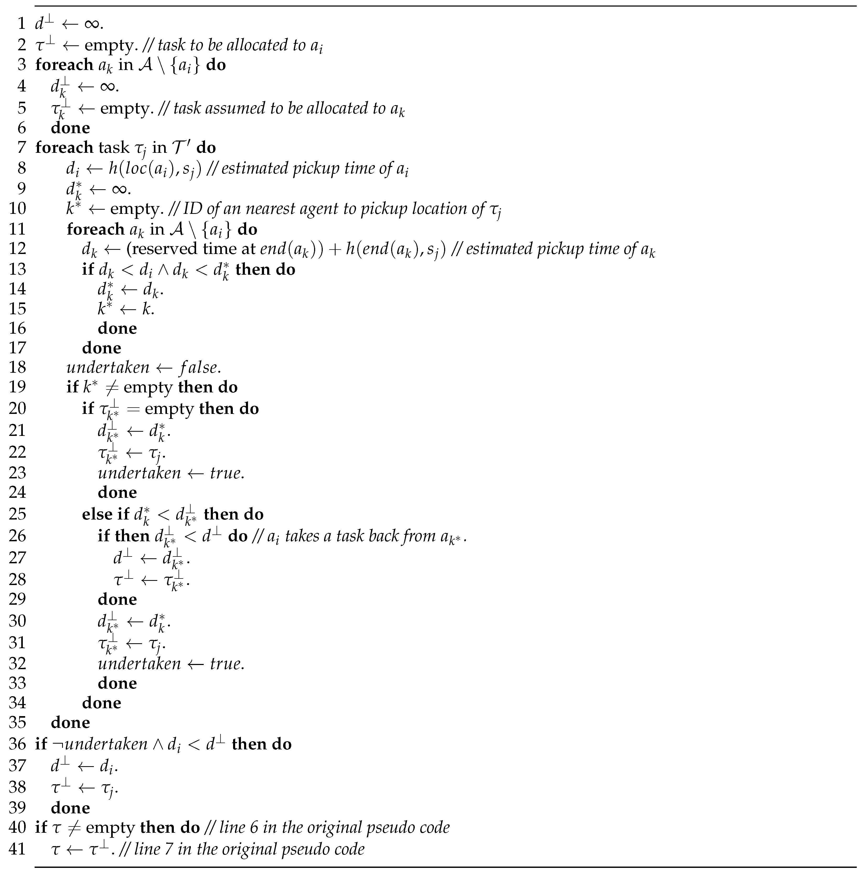
41], we employed the following method considering the balance of computational cost and missing allocations due to a heuristic search. Lines 6 and 7 in
Figure 2 are replaced by the procedure shown in
Figure 7. Here,
denotes the end of agent
a’s path.
As in the previous study in
Section 3.3, if agent
can pick up task
in fewer steps than
, then task
should be allocated to
. Therefore, agent
does not immediately allocate
to it. However, if
finds another task that can be picked up by
in fewer steps than
,
ignores
. We address this issue within a greedy method. In the procedure, agent
leaves task
to agent
if (reserved time at
is less than
, where
denotes the end of agent
a’s path (lines 11–34 in
Figure 7). In addition, agent
assumes that the task will be assigned to
with the minimum estimated pickup time (lines 13–17). If the task nearest
is updated in the search process,
takes the previous task back from
(lines 26–29). Then agent
keeps the nearest one to it in such tasks. If no agent is nearer task
than
, agent
compares
with its kept task to select one of them (line 36).
This is basically a greedy method, but it intends to reduce the missing allocation of tasks in a simple method. While the effect of such a heuristic depends on the problem settings, we prefer this approach.
We selected this heuristic as a relatively simple example of a greedy approach and slightly adjusted it to mitigate the situations of temporarily unallocated tasks due to greedy allocation. In cases of relatively sparse populations of agents in an environment containing obstacles, the accuracy of the estimated pickup time, which is partially based on heuristic distance, will be relatively low, and the task allocation might be incorrect. On the other hand, if the number of agents is sufficient, the time required to pickup each task is expected to be reduced, and the total time until the task is delivered can also be reduced.
4.3. Integration with Paths Containing Arbitrary EPs
Next we integrate a technique that allows paths containing arbitrary EPs (
Section 3.4). Although this technique reduces the length of the paths, the paths containing EPs block the allocation of new tasks whose delivery locations are such EPs. It also needs to modify its selection of EPs to which to retreat so that the EPs locked by reserved paths are excluded.
We improve pathfinding so that it avoids the EPs of the delivery locations of new tasks. This modification allows the traversal paths of agents to only shortcut EPs which are not the delivery locations of new tasks. Since we found that a strict setting that completely avoids such EPs produces relatively long paths, we adopted a heuristic weight value W for the distances to the EPs to adjust the degree of avoidance.
Figure 8 shows an example of agent
’s path that avoids the delivery location of new task
. By inserting such a detour, the delivery location of
is not locked by
’s path, and
can be allocated to an agent.
To manage the information of locked EPs, we employ an additional two-dimensional map corresponding to a warehouse’s floor plan. Agents share this additional map as part of their token, and each vertex/cell v in the map consists of the following variables:
: a counter of the number of paths locking this location;
: a variable recording the start time of an additional staying path of an agent in this location if one exists;
: a counter of the number of waiting tasks whose delivery locations are this location.
The first and second variables, which are related to the reserved paths, are updated when a new path is reserved and when each agent moves on its reserved path at each time step. The last variable is updated when a new task is generated on demand and when a task is allocated to an agent. These are referenced in the additional methods shown above to check the locked EPs. is employed in the task allocation.
In the A* algorithm on a time-space graph, the estimated total path length
for a vertex
at time step
t and an adjacent vertex
is described as follows. It is commonly represented as
where
is the distance (time) from a start vertex to
,
is the distance from
to
, and
is the heuristic distance from
to a goal vertex. We employ the following distance between neighboring vertices.
Here
is employed to evaluate the reservation of a staying agent.
4.4. Integration with Management of Additional Dummy Paths
We next integrate the solution methods shown in previous
Section 4.1,
Section 4.2 and
Section 4.3 and a technique of the additional dummy paths (
Section 3.5). In the basic method, each additional dummy path starts form the last location of a path and ends at a parking location (i.e., mainly non-task EPs). We also address cases where any EP can be used as a parking location and where the number of non-task EPs is less than the number of agents. Therefore, dynamic management of dummy paths is necessary.
For each agent, we introduce a sequence of ’tasks’ that consists of the following:
a pickup-and-delivery or retreat task, if one exists,
optional dummy retreat tasks, and
a stay task if there is nothing to do.
Here we temporarily consider any type of travel paths to be corresponding types of tasks and assume a sequence of tasks has maximum length T. Each agent manages the information of its own task sequence.
First, each agent is assigned to just one from among pickup-and-delivery, retreat, and stay tasks and reserves its travel path as usual. Then dummy paths are added in the following two cases.
(1) If an agent has a pickup-and-delivery or a retreat task, and the end of its travel path blocks tasks that are waiting to be allocated, then a dummy retreat task is added, if possible. Here the dummy path’s goal location is one of the other available (free) EPs. Each agent performs this operation at every time step.
(2) When an agent can select a new pickup-and-delivery task, the agent conditionally adds a dummy path. If the a new task’s delivery location overlaps with a reserved path (excluding its end location), and if there is an available EP to which the agent can retreat, then a dummy path task is added after the allocated task. Next a path is reserved, including pickup, delivery, and retreat locations. To avoid deadlock situations in an environment with a small number of non-task EPs, a pickup-and-delivery task that requires no dummy path is prioritized in the task allocation.
After each agent completes its pickup-and-delivery task or its first retreat task, the agent cancels subsequent retreat tasks and tries to select a new task. However, such a new selected task might be infeasible, since the agent must move from its current location to avoid other agents’ paths that are newly reserved after its own dummy path is reserved. In such cases, the canceled tasks and paths are restored to ensure the consistency of reservations.
We limit the maximum length of each task sequence T and the maximum length of each additional retreat path P to restrict the total path lengths. When there is no EP to which to retreat within a range of P from the current path end of an agent, its related preceding task is not allocated.
4.5. Employing Tasks’ Paths Divided for Subgoals
Finally, we integrate a method that decomposes a single path of a task into multiple paths corresponding to the subgoals of the original task. In our investigation, we simply decompose a task’s path into a sequence of two parts so that the former/latter ends/starts at a pickup location. Therefore, a MAPD problem is modified to a pair of MAPF problems, where each original task is decomposed into pickup and delivery tasks, with a constraint that the decomposed tasks must be assigned to the same agent.
Since this change might introduce different deadlock situations among decomposed tasks, we also modify the conditions in the task allocation.
The pickup-and-delivery tasks are associated to their original task and allocated to the same agent.
Each agent switches between its pickup and delivery modes and can only assign its consistent tasks. Namely, an agent can only allocate the originally same task in its pair of pickup and delivery modes.
The delivery tasks that have been allocated to agents should be prioritized to complete them.
For the last condition regarding the priority of tasks, we simply employ the original task-allocation rule of TP. Namely, the original task with no conflict of pickup and delivery locations is identically allocated to an idle agent as the original TP, although the allocated agent only reserves its pickup path at its first phase. After an agent arrives at the pickup location of its task, it allocates its task again to reserve a path to its delivery location.
The condition of conflict among the agents and the new tasks in line 5 (
Figure 2) is modified as follows. Here each delivery location of a partially allocated task (in its pickup phase) is also considered its reserved location.
For new tasks: s.t. no other agents’ paths in the token and the partially allocated tasks end in or ;
For reallocated tasks: s.t. no other agents’ paths in the token and the partially allocated tasks end in .
In addition, conflicts between the pickup location of each new task and the reserved paths containing EPs are also avoided in the task allocation. Therefore, we also apply a weight parameter of the distance values to avoid the delivery locations of new tasks in the pathfinding (
Section 4.3) to the pickup locations of new tasks.
Although this relatively safe rule might still limit the concurrency of task allocation, we focus on whether there is room to reduce the makespan by partially reserved paths. To avoid complicated situations with this approach, we do not employ techniques of dummy paths in this case.
4.6. Correctness of Integrated Method
The selected additional techniques to be integrated in our approach are correct in the sense of no deadlock situation, and we can combine them without a loss of the correctness of the original solution method TP. Therefore, the resulting methods inherit the correctness of the original TP. Indeed, the integrated techniques substantially complement each other and just need a few adjustments regarding the rules of the endpoints and the reserved paths, as mentioned in
Section 4.1 and
Section 4.3,
Section 4.4 and
Section 4.5. We do not employ a combination of dummy paths and subgoal-division techniques for simplicity in this paper, as shown in
Section 4.5, although we believe that they can be integrated with a slightly complicated adjustment. An understanding of the fundamental property of endpoints also helps develop such integrated solution methods. However, as a baseline case, solution methods still depend on the conditions of well-formed problems excluding those of non-task endpoints. The base line case is also a safeguard for the correctness of the extended solution methods.
5. Evaluation
We experimentally investigated the effects and influence of the integrated techniques. We first present the settings of our experiment, including the benchmark problems and the compared solution methods. Then we report the experimental results that reveal the effect of our approach.
5.1. Settings
We employed the following types of benchmark problems. We evaluated both well-formed problems with non-task EPs and variants without them.
Basic (Envs. 1 and 2 in
Figure 1 and
Figure 6): Env. 1 is based on a well-formed problem shown in a previous study [
17], and Env. 2 is its variant without non-task EPs.
Incoming–storing–outgoing (Envs. 3 and 4 in
Figure 9 and
Figure 10): We modified the basic problems to represent the task flows. Here task endpoints are categorized as incoming, storing, and outgoing EPs. Half of the tasks are incoming tasks, and the other half are outgoing ones. The pickup/delivery location of each incoming task is an incoming/storing EP, and that of each outgoing task is a storing/outgoing EP.
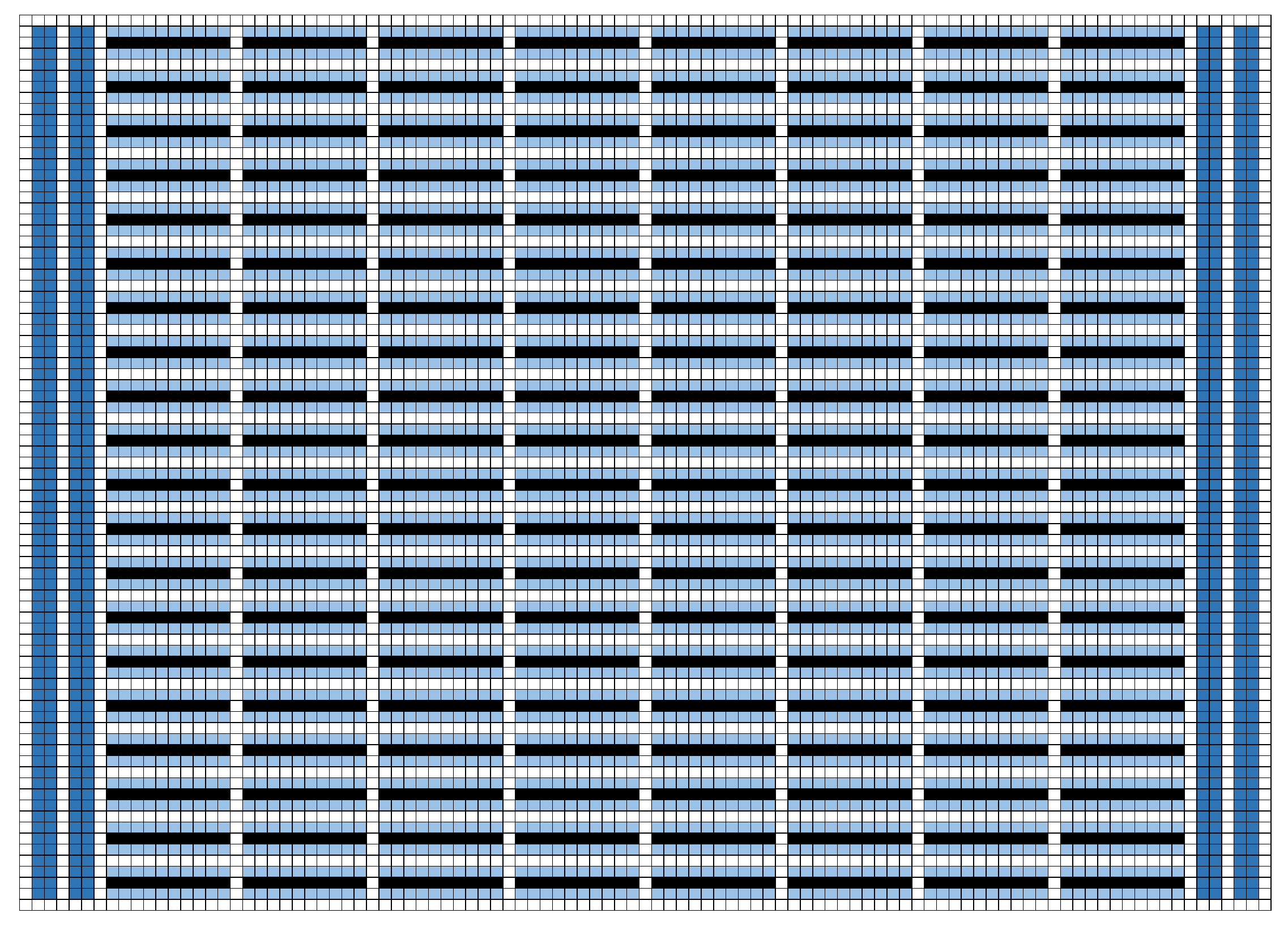
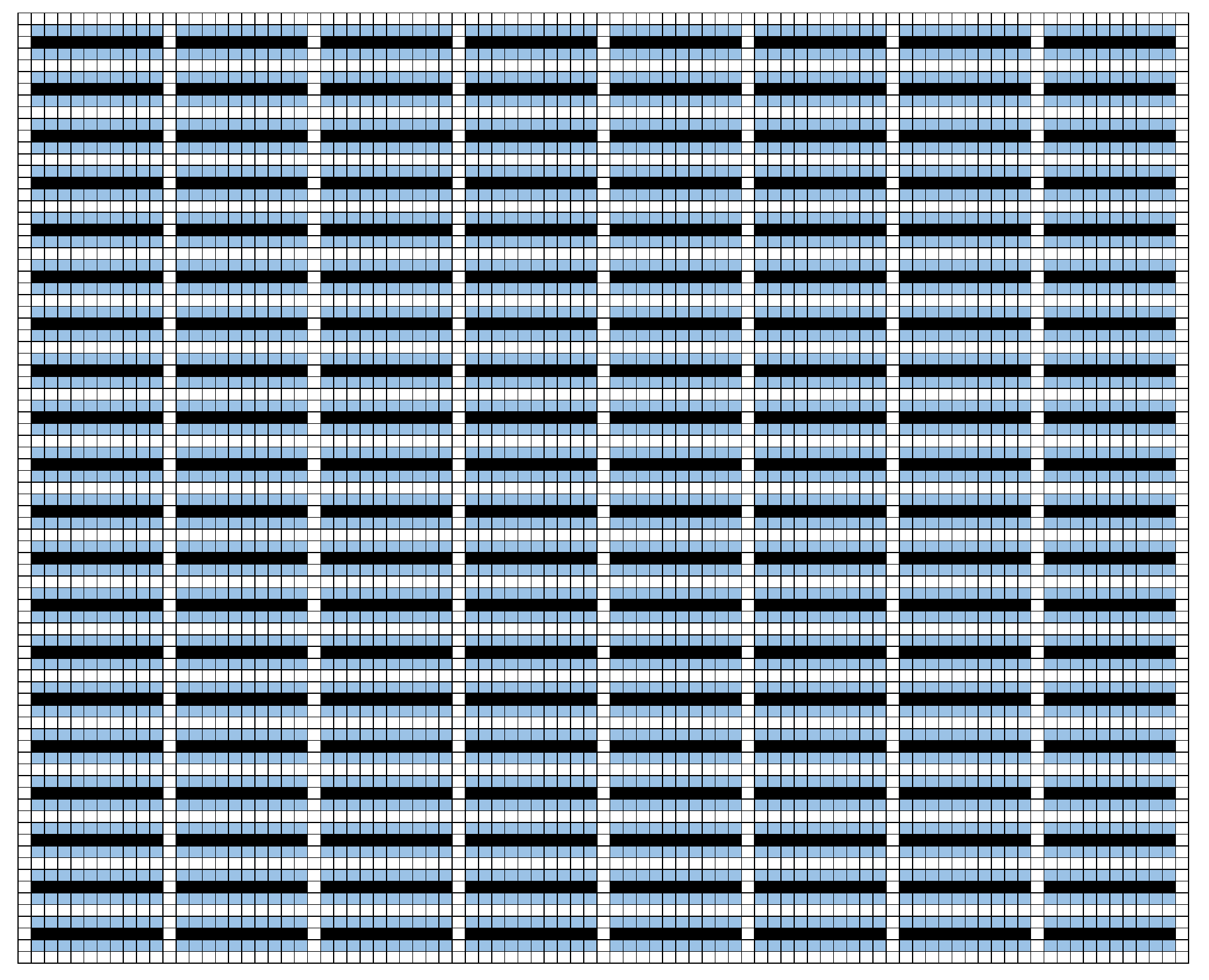
Large-scale (Envs. 5 and 6 in
Figure 11 and
Figure 12): Env. 5 is based on another well-formed problem shown in a previous study [
17], and Env. 6 is its variant without non-task EPs.
The parameters of the environments are summarized in
Table 4.
We varied the number of agents and the task settings. We set the maximum number of agents depending on the number of non-task EPs for well-formed problems and the number of EPs for non-well-formed problems. For the task settings, we selected the total numbers of generated tasks, the number of tasks generated for each time step, and the candidates of the pickup-and-delivery locations depending on the types of maps. At every time step,
tasks were generated, up to the defined total maximum number of tasks. Parameter
affects the possibility of the concurrent execution of the tasks. The initial locations of agents were selected from the non-task EPs for the well-formed problems and all the task EPs for the non-well-formed problems. The initial locations of the agents and the pickup-and-delivery locations of the tasks were randomly selected from their corresponding cells/vertices with uniform distribution. The parameters of the tasks and the agents are summarized in
Table 5.
We evaluated our selected additional techniques below by incrementally combining them. The possible full combinations of them in our result are shown in
Table 3. We selected a subset from the possible full combinations, as shown in the following tables of results.
We evaluated the makespan (MS) to complete all tasks, the service time (ST) to complete each task, and the computation time (CT) per time step. The units for MS and ST are logical time steps, and the units for CT are milliseconds. Note that the computation times include some disturbances in a computation environment.
The results over ten runs with the random initial positions of the agents were averaged for each problem instance. We employed a computer with g++ (GCC) 8.5.0 -O3, Linux 4.18, Intel(R) Core(TM) i7-9700K CPU @ 3.60 GHz, and 64 GB memory for the experiment. The maximum memory usage was within 220 MB for large-scale problems.
Our experimental implementation of algorithms focuses on an investigation of the simulation results and employs several statistical processing and cache data of maps. There are opportunities for improving them for practical implementations.
5.2. Results
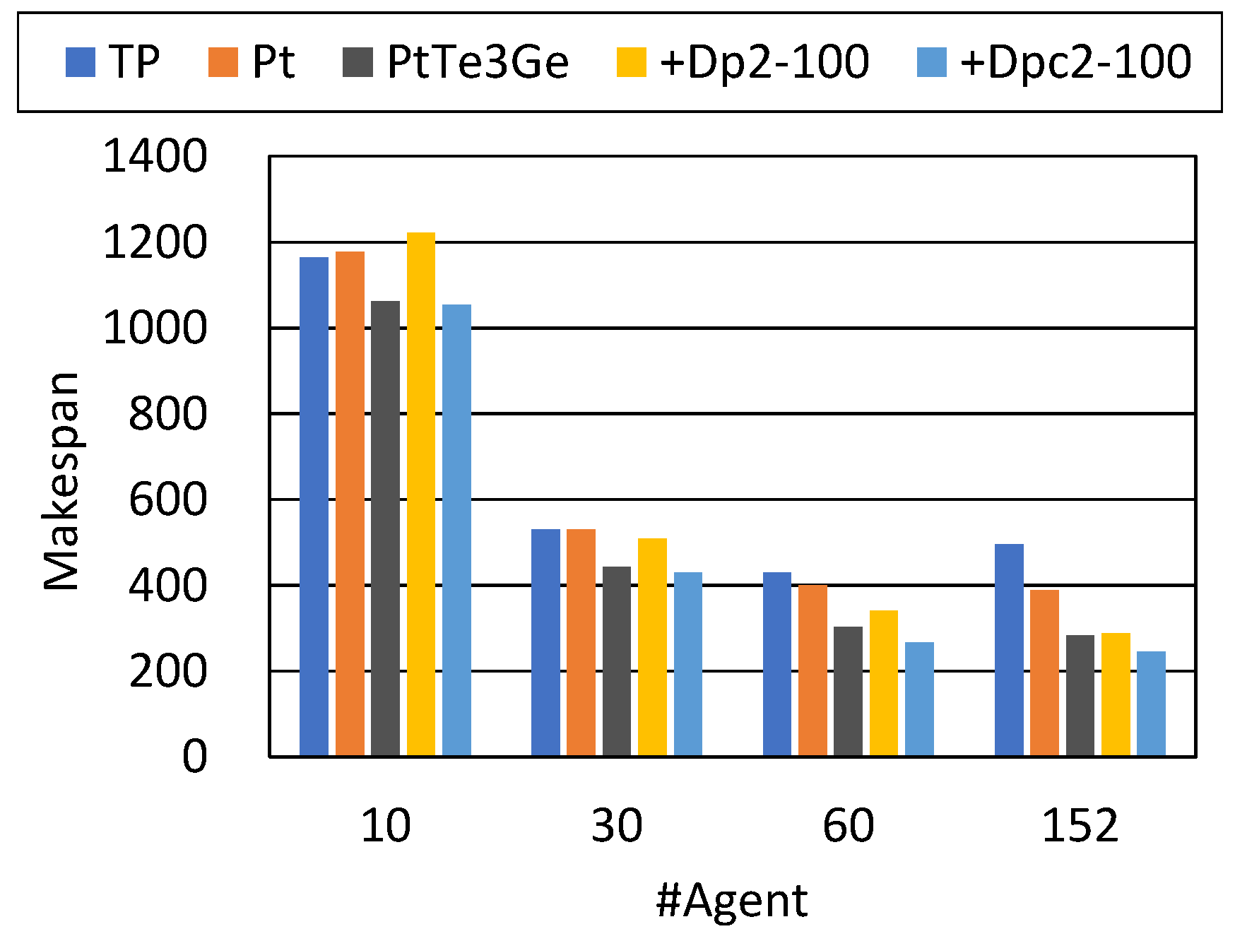
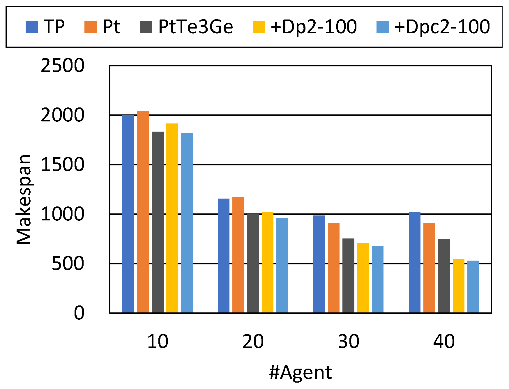
The best value in each setting is emphasized in bold. We discuss the effect of integrated techniques with the results. Pt based on the estimated pickup times reduced the actual pickup times when a sufficient number of agents cover a whole map without congestion, and it also reduced the makespan and the service time (, 60 agents).
Te reduced the makespan and the service time by allowing shorter paths through EPs, although it increased the number of temporarily locked EPs. In these settings, the results were identical for the cases with/without Ge because there were enough EPs for the agent to retreat to.
Dp and Dpc improved the results by increasing the concurrency of tasks in the situations where the tasks were continuously assigned to a relatively large number of agents (, 60 and 152 agents).
For such problems, Dp and Dpc were relatively competitive with PIBT (Table 2 in a previous work [
12]).
In these cases, SG completed all the tasks without deadlock situations, although the makespan and the service time slightly increased in most results. This overhead was caused by the waiting time for the task allocations divided into subgoals as well as some increments of the length of the divided paths.
Table 8 and
Table 9 show the results with different parameter settings. For weight parameter
W imposed on the distance to the EPs with waiting tasks, a relatively small value achieved a good trade-off between the avoidance of such EPs and the total length of the detour route.
To avoid excessive locking of EPs by dummy paths, appropriate settings appeared to emerge for the maximum number of tasks T, including dummy retreat tasks, and the maximum length of dummy paths P. In these results, a smaller value of T and a sufficiently larger value of P were relatively better.
Table 10 and
Table 11 show the result for Env. 2. The absence of non-task EPs in this setting increased the trade-offs between the effect and overhead in the additional methods when the population density of the agents is relatively high. When the number of agents was not excessive, a solution method based on Ge competed with those in similar problems with non-task EPs.
Although Dp and Dpc reduced the makespan and the service time in appropriate settings, their overhead also increased with the number of agents. Particularly in the excessively dense case of 199 agents, there was almost no room for the effect to reduce makespan and service times by the methods.
Table 12 and
Table 13 show the result for Env. 3 (incoming–storing–outgoing). Although this environment resembles Env. 2, there are incoming and outgoing EPs on both the left and right sides. Non-task EPs for well-formed problems are placed in the top and bottom areas. One endpoint of each task is an incoming or outgoing EP, and this situation relatively lengthens the travel paths of the agents.
In this case, the combinations of Pt, Te, Ge, and Dp/Dpc well reduced the makespan and the service time. PtTeGeSg slightly reduced the makespan more than its baseline method PtTeGe in the case of and 40 agents, while there is still some overhead in service times. Although this number of agents is maximum (i.e., the number of non-task EPs), below we confirm a similar result in an environment without non-task EPs.
Table 14 and
Table 15 show the result for Env. 4. Although the non-task EPs were eliminated from the previous setting in this environment, the result resembles that of Env. 3.
In this result, PtTeGeSg slightly reduced the makespan more than PtTeGe in the case of sixty agents. We saw such a trend in the cases of 40 and 50 agents. Since these problem settings often generate long travel paths of agents in opposite directions, the effect of Sg appeared to be revealed in the cases of relatively dense populations of agents. However, no such result surfaced in the extremely dense case (199 agents).
Table 16 and
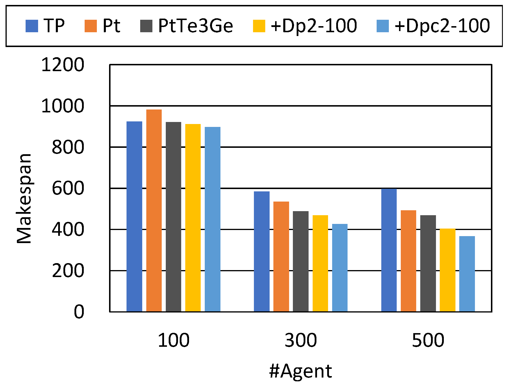
Table 17 show the result for Envs. 5 and 6 (large-scale). The populations of the agents were relatively sparse, and the effect of the additional methods was also relatively small. However, a combination of additional methods reduced the makespan and the service time, particularly for 300 and 500 agents. In the latter case, PtTeGeSg slightly reduced the makespan more than PtTeGe in average.
A major issue here is the overhead of the additional methods in the computation times, although there are chances to improve our experimental implementation, as discussed in
Section 5.1. One such overhead comes from our implementation of Pt that considers the estimated pickup times of the other agents in the task allocation. Since our current version evaluates all the agents and all the allocatable tasks in the task allocation process, it was affected by the numbers of both agents and allocatable tasks.
Another overhead was due to the canceling and restoring of the dummy paths in Dpc. Our current version searches for the possibility of task allocation with the pathfinding of each task’s path after a dummy path of an agent is temporarily canceled. The dummy path is restored if the task allocation fails. Our current version was also affected by the number of agents and the size of the environments. In practical cases, a large warehouse’s map might be divided into sub-areas to mitigate the computational cost of the solution methods.
In summary, we found that the redundancy in well-formed problems and solution methods based on EPs can be reduced by appropriately combining and setting our selected additional techniques.
Pt was effective in situations where a certain number of tasks to be assigned were waiting in an environment with a sufficient number of agents.
TeW was effective in most situations, although there were some trade-offs regarding the number of locked/unlocked EPs.
Ge was a useful option that reduced the number of non-task EPs.
DpT-P/DpcT-P was effective in situations with a sufficient number of free EPs to which agents can additionally retreat.
Although opportunities remain for improving the current SG to reduce redundant waits for the decomposed task assignments, some results revealed the effectiveness of this technique.
The incremental combinations of Pt, Te, and Dp/DPc were basically effective. However, there are inherent trade-offs among the methods, especially in situations where the population density of the agents was high and the number of free EPs was relatively small.
Although Dp and Dpc required relatively large computational cost to manage the dummy tasks/paths, the experimental implementation of the methods can be improved. Additionally, some parts of the computation can be performed while the agents are on their journey, and their moves typically take a longer time than the computation.
Figure 13,
Figure 14 and
Figure 15 show the makespans in a major part of our result. We extracted them from the cases with non-task EPs, to include the base TP algorithm. Although the result revealed several trade-offs, a full combination ’+Dpc2-100’ was effective with sufficient numbers of agents.
6. Discussion
The effects of the additional integrated methods are basically complementary. The Pt method that considers the estimated pickup times affects the task allocation process. Te, which allows travel paths of agents to contain arbitrary EPs, reduces the path length. Dp employs additional dummy paths and resolves the conflict among an end of an agent’s path and a delivery location of a task waiting to be allocated. Ge, which accepts map setting without non-task EPs, reduces the space of maps, and Dpc, which conditionally cancels dummy paths, is particularly important in such narrow maps. Regarding Te and Dp, an agent avoids the delivery locations of new tasks in its pathfinding process with our improved Te, and Dp resolves such conflicts after the agent’s path is reserved.
We describe some directions to enhance the employed techniques. Our Pt method that considers the estimated pickup times in the task allocation process currently evaluates all the agents and all the allocatable tasks; it requires relatively large computational cost for large-scale problems. Some elements of the agents and tasks that are evaluated in the process can be eliminated considering the areas in a large map.
For the Te method that allows the travel paths of agents to contain arbitrary EPs, we introduced weight values that are added to the distance values in the pathfinding to avoid the delivery locations of new tasks, and the experimental result revealed the room to adjust the weight parameter for situations (
Table 8). The insertion of such detour paths might be controlled by evaluating the density of idle agents in local areas in a certain period of time.
Our current Sg method, which divides a task’s path was simply applied to all the tasks as an investigation to integrate it with several heuristic add-on methods. To bring out its effect, the division could be conditionally applied to tasks whose pickup-and-delivery locations are separated areas in a map, while the integration of different task allocation rules is necessary for decomposed and non-decomposed tasks.
The solution methods based on TP complete all the tasks generated on demand if a finite number of tasks are generated. However, there is an issue of fairness among tasks waiting to be allocated, and a starvation situation can be a problem in the task allocation. This drawback can be addressed with an approach using the threshold or the priority values to consider the waiting times of tasks. Generally, there is a trade-off between efficiency and fairness. We mainly focused on efficiency in the makespan to complete all the tasks.
Although we employed several techniques in the solution methods to partially relax the conditions of the well-formed MAPD problems, the maps of the warehouses themselves remain restricted by some fundamental conditions regarding endpoints. The solution methods still depend on the conditions as a safeguard. The challenges of mitigating the limitations of maps will require greater consideration of the conditions for avoiding deadlock situations within time windows.
In summary, excluding an experimental version of subgoal division of each task, the full combination of our selected techniques with several improvements resulted in the best performance in most cases in the sense of makespan. We recommend this solution method in our evaluated methods except for excessively dense agent populations. When computational overhead is an issue due to dense agent populations, a technique with dummy paths can be omitted in turn for trade-offs with other performances.


