1. Introduction
Air pollution, as a serious environmental and social problem, has received a lot of attention globally [
1,
2,
3]. According to a report published by the World Health Organization (WHO) on global air quality in 2022, PM
2.5 is on the rise globally and poses a serious threat to people’s health, including respiratory infections, pneumonia and lung cancer [
4,
5,
6]. In particular, air pollution caused by crop residue burning in Northeast China is more intense than that of other regions in recent years [
7]. The Air Quality Index (AQI) is used by many developed and developing countries around the world to assess air quality, considering the composition of particulate matter, gaseous pollutants and other factors. A high AQI indicates that people’s health is at risk and that government policies are needed to improve air quality [
8]. Therefore, the real-time monitoring and prediction of air quality is an important basis for promoting the sustainable development of a country.
At the same time, meteorological conditions, living habits, transportation, industrial activities, and environmental regulations all have different impacts on air pollution [
9,
10,
11]. Emissions of particulate matter 2.5 (PM
2.5), particulate matter 10 (PM
10), carbon dioxide (CO
2), sulfur oxides (SO
X), nitrogen oxides (NO
X), ozone (O3), and ammonia (NH
3) are exposed to the atmosphere from these activities, thus contributing to the creation of climate extremes. Such negative influences include global warming, acid rain, smog, and aerosols. As a result, air quality research has moved away from single-variable predictions to a combination of factors that increase the interpretability of the predictions [
12,
13,
14,
15].
Looking back at past studies, researchers have created prediction models based on physical, statistical, machine learning and deep learning. Physical models can obtain theory-based accuracy by simulating physical processes such as the production and diffusion of pollutant gases [
16,
17]. However, their strict assumptions, specific environments and long-term observations make the models severely limited in their application. For that reason, statistical models have emerged and have been applied to plenty of fields for forecasting. As statistical science advances, more and more statistical forecasting methods are surfacing, including Seasonal-Trend decomposition using LOESS (STL), Exponential Smoothing State Space Models (ETS), Seasonal Autoregressive Integrated Moving Average (SARIMA), Holt–Winters Exponential Smoothing (HWES), etc. Statistical models based on data overcome these problems and improve forecastingaccuracy by performing complex calculations and statistics on the data [
18,
19].
However, these traditional methods have some limitations. First, feature extraction is a challenge and traditional methods often require manual selection and extraction of features, which can lead to information loss and model performance degradation. Second, traditional methods tend to assume spatial and temporal smoothness, which fails to capture the nonlinearity and time-varying character of air quality data. In addition, traditional methods have a limited ability to handle large-scale multidimensional data and are difficult to deal with complex spatial and temporal relationships.
Therefore, machine learning based air pollution forecastingsystems are considered as an option to produce better results. In recent years, one of the branches under the development of machine learning, Deep Learning (DL) has become quite popular and effective forforecasting, and for its ability to efficiently process data and capture influencing relationships [
20,
21,
22]. In particular, Convolutional Neural Networks (CNNs) are widely used in image processing with their excellent feature extraction capabilities, while Bi-directional Long Short-Term Memory Networks (BILSTMs) are able to efficiently capture long-term dependencies in time series data. The combination of these two models is shown to have great potential in air quality prediction [
23,
24,
25]. Du et al. used one-dimensional convolutional neural networks (1D-CNNs) and bi-directional long- and short-term memory networks (Bi-LSTMs) to construct a joint hybrid deep learning framework to learn the spatial-temporal correlation characteristics and interdependence of multivariate air quality-related time series data [
26]. In a multi-temporal, multi-site prediction experiment of Beijing air quality designed by Yan [
27], CNN-LSTM and LSTM are shown to have better performance than CNN and BPNN and exhibit the same superiority in both seasonal and spatial-based prediction. Qi proposed a Deep Air Learning (DAL) model solving the three problems of interpolation, forecastingand feature analysis through a feature selection model and semi-supervised learning embedded into different layers of a deep learning network [
28]. Using 96 consecutive hours of nonlinear smog data from four cities, Wang et al. verified that a two-layer model prediction algorithm based on long-term short-term memory neural networks and gated recurrent units (LSTM&GRU) can make better predictions [
29]. By combining CNN and BILSTM models, complex patterns and regularities in data can be learned automatically. Moreover, with the development of deep learning, more and more advanced forecasting models were applied to time series forecasting. Among them, auto-encoder models have been popular for their better performance, which utilized encoders and decoders to reconstruct the raw data [
30]. Apart from that, attention mechanisms gained more popularity. Bahdanau used attention mechanisms to complete the task of machine interpretation for the first time [
31]. Then, various types of attention mechanisms took place, such as Co-Attention networks [
32], Self-Attention networks [
33] and Recurrent Attention networks [
34].
In addition, plenty of combined and hybrid forecasting models were constructed to achieve better accuracy in terms of time series forecasting. Generally, the modeling techniques propose hybrid models that include the following aspects: data decomposition, data convolution, feature selection, ensemble modeling and model optimization. For example, Huang et al. proposed an EEMD-GPR-LSTM method for forecasting, in which CPR and LSTM were treated as inherent modes after ensemble empirical mode decomposition was applied to the original data [
35]. Different data decomposition methods were combined with the ensemble module, thus constructing various hybrid models, such as the EWT-LSTM-Elman model [
36], the DBSCAN-SDAE-LSTM model [
37], etc. Moreover, the introduction of model optimization boosts the variegation of forecasting models. Liu et al. designed a VMD-SSA-LSTM-ELM, in which SSA was proposed to extract the potential trend information between all subsections.
Spatiotemporal correlation is a pivotal factor in air quality studies. Spatiotemporal correlation refers to the correlation that exists between changes in air quality in time and space [
38,
39,
40]. In urban agglomerations, changes in air quality often depend not only on the city’s own pollution sources and meteorological conditions but are also influenced by the surrounding cities. For example, if other cities surrounding a city have significant industrial emissions or meteorological conditions that are not conducive to the dispersion of pollutants, the air quality of that city may be negatively affected [
41]. Such interactions can be revealed by the analysis of spatiotemporal correlation.
The study of spatiotemporal correlations can be carried out through a variety of methods. One common method is to use air quality monitoring data for spatiotemporal analysis. By collecting air quality data from multiple cities and combining them with meteorological data and pollution source data, it is possible to analyze air quality trends and interrelationships between cities. This kind of analysis can help us understand the air quality transmission paths and influencing factors in city clusters. Another approach is to use mathematical models to simulate and predict the spatial and temporal correlation of air quality. Mathematical models can be based on physical principles and statistical methods to predict air quality changes between different cities by modeling air quality transport in urban agglomerations. Such models can take into account factors such as pollutant emission sources, meteorological conditions, and geographic features to more accurately predict air quality changes and interactions in urban agglomerations.
Currently, many studies have used social neural networks to analyze air quality interactions. However, few scholars pay attention to taking the interactions of different city nodes into account in the forecastingmodels or forecastingsystems over a period, which attempts to apply qualitative methods to explain quantitative issues. Network correlation studies have long widely been used in finance, biology and climatology, among others [
42,
43,
44,
45,
46]. Wang et al. [
47] proposed a linear combination of correlation network topological indices to measure the correlation between oil-dependent countries. Du et al. [
48] considered the effect of time lag and optimized the oil import correlation network using seepage analysis, which significantly improved the accuracy of the original model and better captured the riskiness of crude oil imports. The study of network correlation can help us analyze and understand the structural characteristics of networks. By studying the connection patterns and topology between nodes, we can reveal the clustering phenomenon, small-world nature, scale-free distribution, and other features in the network. This is important for understanding the organizational principles of networks, the importance of nodes and the mechanisms of information dissemination. In this paper, we apply it to air quality, and by studying the interactions and information transfer between nodes, we can find out the existence and evolution of air pollution, so as to forecastand control the behavior of the complex system and provide a scientific basis for decision making and risk assessment.
Above all, the motivation of this manuscript is to make a contribution to the advancement of a combination of air quality forecasting modeling and social network analysis in urban agglomerations. Based on the above point of view, this paper proposed a complex system to realize accurate short-term forecasts and online analysis in cluster areas, helping the monitoring and prevention of air pollution. Although related works have explored the various objective factors that are relevant to air pollution, there are few articles that considered public emotions could also reflect the change in air pollution. Thus, our work addresses this limitation by introducing subjective factors to assist forecasting through text sentiment analysis. Unlike single feature selection strategies which solely concentrate on the correlation between variables, our work attempts to balance the extent of feature selection and result fusion. This approach could not only ensure the comprehensiveness of the feature selection effort but avoid the neglect of information of relatively weak importance. Moreover, this paper also proposes an optimal CNN-D-LSTM which performs better to some extent than before in forecasting and utilizes social network analysis to help understand the spatial correlation and dynamic change in the urban agglomerations. By doing so, this paper provides reliable and robust short-term forecasting together with a dynamic social analysis method for cluster air pollution problems.
The main contributions of this paper could be summarized as follows:
- (1)
Text sentiment analysis is performed to explore public emotions related to air quality, which is then introduced to the construct of explanatory variables. It is verified that adding public emotions improves the performance of the forecasting model.
- (2)
A feature processing strategy based on multiple feature selection methods and result fusion is innovatively proposed to solve the problem of difficulty in extracting features from air pollution data.
- (3)
A CNN-D-LSTM is constructed by adding a DenseNet, which greatly reduces the probability of parameter explosion and improves the ability to extract useful information automatically, thus contributing to the superiority of forecasting performance.
- (4)
Social network analysis is introduced to improve the interpretability of air pollution correlations in urban agglomerations. Moreover, the additional social analysis is conducive to dynamic monitoring and timely policy-making.
- (5)
The combination of forecasting and social analysis could be expanded to many other fields for helping the exploring of cluster change and other applications, which is also an advancement of spatial correlation analysis.
The rest of this paper is developed as follows:
Section 2 introduces the overview of our constructed system and the detailed introduction and rationale of the methods, while
Section 3 shows the information about collected data, the preprocessing of raw data, and the results of simulations and experiments. Moreover,
Section 4 is the discussion of this paper, in which some modeling tests were conducted. Ultimately, in
Section 5 some conclusions were drawn from the analysis in the above parts, including main conclusions, academic implications, managerial significance and future research directions.
2. Methodology
2.1. Problems and Motivations
Accurate air quality forecasting can serve as an auxiliary technique to explore the spatial characteristics of urban agglomerations in terms of air pollution. Based on forecasting modeling, our goal was to make feasible recommendations for air pollution prevention and control, from a spatial distribution perspective. Thus, we proposed a hybrid deep learning model, which integrated text sentiment analysis and a CNN-D-LSTM model relying on prominent features processed by adaptive feature engineering. Then, a complex network for spatial correlation analysis was utilized. The details of the methods used in this manuscript were introduced as follows and the overall scheme is shown in
Table 1.
2.2. Text Sentiment Analysis
Text sentiment analysis, applied to stock prediction, product review and other fields, is defined as extracting emotions using NLP, statistics, or machine learning, which puts insight into text [
49]. When it comes to air quality forecasting, a potential correlation between public emotions and air quality was assumed to exist. In other words, public emotions might play a role in air quality forecasting.
To obtain public emotions about air quality, this paper designed a framework as follows:
Step 1: First, identify the mainstream platforms or forums that are geared towards this based on the volume of users, and then utilize crawling techniques to obtain comments on air quality from these platforms.
Step 2: Jieba’s word separation algorithm was utilized in text information preprocessing, including deactivation and text vectorization. In this case, the implementation of the word separation algorithm is performed as follows:
where
n denotes the number of word vectors and
d denotes the dimension of the word vector. Thus, a piece of text is transformed into word-vector form in terms of words, subsequently forming a word-vector matrix
.
Step 3: The word vectors were then subjected to feature extraction and sentiment classification to identify keywords that reflect public emotions.
Step 4: Based on the above keywords, a Baidu search index corresponding to the date that the air pollution data were obtained and used as a reflection of public sentiment. Respectively, the Baidu index includes both computer and mobile.
2.3. Feature Processing
Feature processing usually includes feature extraction and feature selection. It was widely used in the forecasting field, especially playing a key role in machine learning and data mining, which could avoid dimensional explosion and improve model accuracy [
50].
Given that different types of feature selection approaches have their own advantages and disadvantages, this paper proposed a feature processing method based on multiple feature selection strategies and result fusion.
The basic scheme of feature selection could be described as follows:
(1) Filter algorithm: To generate effective influencing factor subsets for air quality forecasting, it is important to filter less crucial features. On one hand, appropriate feature filtering can effectively avoid the dimension explosion problem in the subsequent substitution of machine learning models, which is conducive to improving model adaptability. On the other hand, in the case of different urban agglomerations, there may be differences in the factors influencing air quality, and adaptive filtering can help to find the key influencing factors. In this study, the grey correlation analysis served as a filter algorithm to eliminate variables of lower importance, while significant features were selected. The corresponding formula is as follows:
Given that
donates a series of feature subsets:
where
i donates the number of feature subsets and
donates the corresponding feature matrix while
n represents the total number of feature matrices.
For
, the grey correlation between
was expressed below:
where
represents the minimum difference between the two levels of the characteristic series and
represents the maximum difference between two levels of the characteristic series.
(2) Embedded algorithm: After the feature subsets are acquired, it is essential to evaluate these features from another perspective. In this paper, LASSO was utilized as an embedded algorithm. LASSO obtains a more refined model by constructing a penalty function such that it compresses some of the regression coefficients. Moreover, it forces an absolute sum of the coefficients to be less than some fixed value, while it sets some of the regression coefficients to zero [
51].
Consider the following multiple regression model
. The
n-dimensional explanatory vector
is defined by
in which
, thus forming the design matrix of order
, while
donates the respond vector. Typically, the least squares method (OLS) is applied to solve the multiple linear regression equation to obtain the least error
Q and the regression coefficients
, which are given by:
However, numerous parameters increase the complexity of the model, for this reason, this paper introduces a penalty term [
52], thus
can be defined as:
Through the combination of the Filter algorithm and Embedded algorithm, the most important variables were selected. Despite that, the number of features selected also might be larger, and affect the efficiency of the forecasting model, thus this paper conducteda necessary result fusion.
(3) Result fusion: Principal component analysis (PCA) is known as a classic method for high-dimensional data preparation, especially in the field of explanatory data analysis and forecasting model conducting [
53]. It specializes in data degradation, which not only preserves key information but also removes unanticipated noise [
54]. The PCA algorithm is executed as shown in
Table 1.
2.4. Forecasting Module
Owing to the strength of LSTM in handling the problem of long-term dependencies, it has been widely used in the application of energy and medicine [
55]. Previous experiments in related fields have confirmed the advantages of LSTM models in time series forecasting, with a better ability to extract past information features than other models [
56,
57]. In addition, the CNN layer has a strong ability to capture the potential feature information, which could assist in the forecasting of LSTM.
Previous studies have proved that CNN-LSTM not only has the ability to mine the potential information for forecasting but also behaves well in the work to memorize and process past information. However, in predicting the air quality of city clusters when considering spatial correlations of air pollution, traditional CNN-LSTM does not perform as well as expected. Therefore, this paper proposed CNN-D-LSTM by adding a DenseNet to the former structure as shown in
Figure 1.
2.4.1. CNN Layer
CNNs have a wide range of applications, such as computer vision and feature extraction, for their excellent processing of image and video data. The core idea of CNNs is to synthesize the use of convolutional, pooling and fully connected layers.
In the beginning, the input data pass through a convolutional layer and near features are extracted using filter sliding.
where
is the input 1-D feature matrix,
represents the activation function used in this layer, and
represents the convolution kernel filter at the
l-th position. Finally, after constant error
correction by the convolutional layer, outputs after convolution are gathered.
The above equation carries out a maximum pooling step that reduces the network complexity while simplifying the computation.
where
represents the features extracted by the CNN layer, which are also the inputs of the LSTM layer.
2.4.2. LSTM and Output Layer
In the LSTM layer, there are three gate structures that play a key role: input gates, forget gates and output gates. Among them, the input gate plays the key function of memorizing new information, acting through the sigmoid function:
where
refers to the input feature at
t-th time while
donates the output of the input gate. Specifically,
represents the corresponding weight of the input gate,
is the bias vector, and
refers to the activation vector of the last time
t − 1.
Subsequently, the outputs of input gates turn into the inputs of forget gates, and the gates determine the information that needs to be forgotten from previous memories. It outputs a value between 0 and 1 by means of the above sigmoid function that indicates how much information is retained in each memory unit.
As the output of the forget gate approaches 0, it indicates that more information needs to be forgotten and as it approaches 1, it indicates that more information needs to be retained.
Ultimately, the outputs of forget gates enter output gates. The output gates determine how the information stored in the memory is passed on to the next time step or output layer. It receives the current moment information on the one hand and processes the pre-memorized information on the other hand, combining the two to obtain the corresponding output value.
where
and
donate, respectively, the output value of the LSTM layer at
t-th and (
t − 1)-th time while
refers to the stored memory at
t-th time.
2.5. Social Network Analysis
Social network analysis (SNA) is considered to be a method for illustrating and analyzing certain phenomena from a community, such as carbon emissions, economic development, and so on. In this paper, SNA was introduced into air pollution analysis, in which each node represents a city and the linkages symbolize the relationship between each two cities [
58].
In the investigation of air pollution urban agglomeration linkage network, a correlation network was constructed among city nodes first. The aim was to explore the dynamics and interactions of air pollution in urban agglomerations. However, there exists a shortcoming of relying solely on a holistic perspective, which will lose some significant information. Thereby, this section used the idea of sliding windows determined by window size and moving steps. Considering the characteristics of air pollution, this paper set a sliding window size of 7 days with a moving step of 1 day. To make this relationship distinct, a time lag effect function was utilized as follows:
where the fluctuation of the feature subset with respect to average
was represented by
where
is the mean value of
, and
was defined similarly. Respectively,
and
represent the overall degree of series fluctuation.
It is worth mentioning that , the time lag, belongs to the internal , where . According to the absolute value of the cross-correlation function , is defined; it reflects the direction between nodes i and j. That is to say, when the direction of these two cities is from node i to j, and when the direction opposes. When , these two cities are indirectly connected.
The weighted adjacency matrix at time
t is defined as:
where
donates the threshold value, which is determined by the mean value of
in this paper. The set of
is to simplify the correlation network to aid the subsequent analysis.
2.6. Evaluation Matrix
To assess the effectiveness of the proposed forecasting system, this paper constructed a suitable and comprehensive evaluation system based on previous studies in the field of forecasting. These evaluation indicators could be divided into two categories: absolute and relative error indicators.
For absolute error, the frequently used indicators are mean absolute error
and root mean square error
, which could be expressed as follows:
where
refers to the actual value of AQI at
t-th time and
donates the forecasted value at the corresponding time. In general,
and
reflects the magnitude of the deviation of the model’s predictions from the true value in absolute numbers. However, this type of indicator is susceptible to factors such as the scale of measurement, thus losing its evaluative accuracy. Thus, relative error indicators were utilized to overcome this shortcoming including:
where
donates the Pearson correlation between the actual and forecasted value in the proposed forecasting system, which evaluates the prediction error in terms of the whole series. The better
and
is, the higher the prediction accuracy and the better the model fits.
3. Case Study
This section reveals the evaluated performance of the forecasting module and empirical analysis by SNA. This contains the data details including the data source and its description, data preprocessing, the designed experiment simulations and related results along with the interpretations and conclusions drawn from it.
3.1. Study Area and Data Description
In recent years, air pollution in the Northeast has received widespread attention. Given its development pattern and geographic location, it is particularly important to provide practical advice on air quality forecasting and joint prevention and control. In this paper, taking the urban agglomeration as a unit, the typical Harbin–Changchun urban agglomeration was chosen as the research object (Detailed description listed in
Section S1 in Supplementary File). The position information of the chosen study area is shown in
Figure 2.
This agglomeration consists of 11 cities, respectively, located in Heilongjiang Province and Jilin Province, whose air quality is represented by AQI, as shown in
Table 2. The raw data of AQI are daily and have a duration of 2192 days, dating from January 2015 to December 2019, which can be sourced from websites
http://www.tianqihoubao.com (accessed on 13 May 2023).
From the above description of the AQI in the Harbin–Changchun urban agglomeration, some conclusions could be made:
(1) It is obvious there are a lot of missing values in the raw data of AQI, amounting to almost 2.05%. The reasons causing that source from a number of factors: regular instrument maintenance, program adjustments, loss of data, etc. Necessary measures should be taken to tackle this problem, preventing its effect on the subsequent forecasting and analysis.
(2) The extremes in the raw data deviate far from average urban air pollution conditions and cannot be underestimated. Thus, certain extreme value detection and correction methods are necessary.
(3) There are significant differences in the air pollution status of the cities in the urban agglomeration in terms of mean, standard deviation and extreme values. For example, the average level and fluctuation of air pollution in Harbin is highest while its maximum is lower than in Songyuan, and the maximum in Yanbian is lowest while the average pollution level is more severe than in Songyuan. Therefore, rational community construction can reduce inter-city air pollution differences and may help in urban agglomeration prediction.
(4) With the help of skewness and kurtosis metrics, it is easy to confirm that the raw data of AQI are non-normal and traditional time series modeling methods are difficult to implement.
In addition to the AQI, this paper introduces other variables to aid in prediction. Eighteen variables ranging from different fields were finally selected, containing: (1) Air pollutant concentrations: PM
2.5, PM
10, SO
2, NO
2, CO and O
3; (2) Meteorological data: Cumulative daily precipitation, cumulative daily light, average air temperature, average air pressure, average wind speed, and average humidity; (3) Public emotions: Haze Index and Environmental Pollution Index, including mobile, computer and total indices. The length of these variables is the same as that of AQI. Air pollutant concentrations are collected from the website
http://data.cma.cn (accessed on16 May 2023) while the data representing public emotions are from the website
https://index.baidu.com (accessed on16 May 2023).
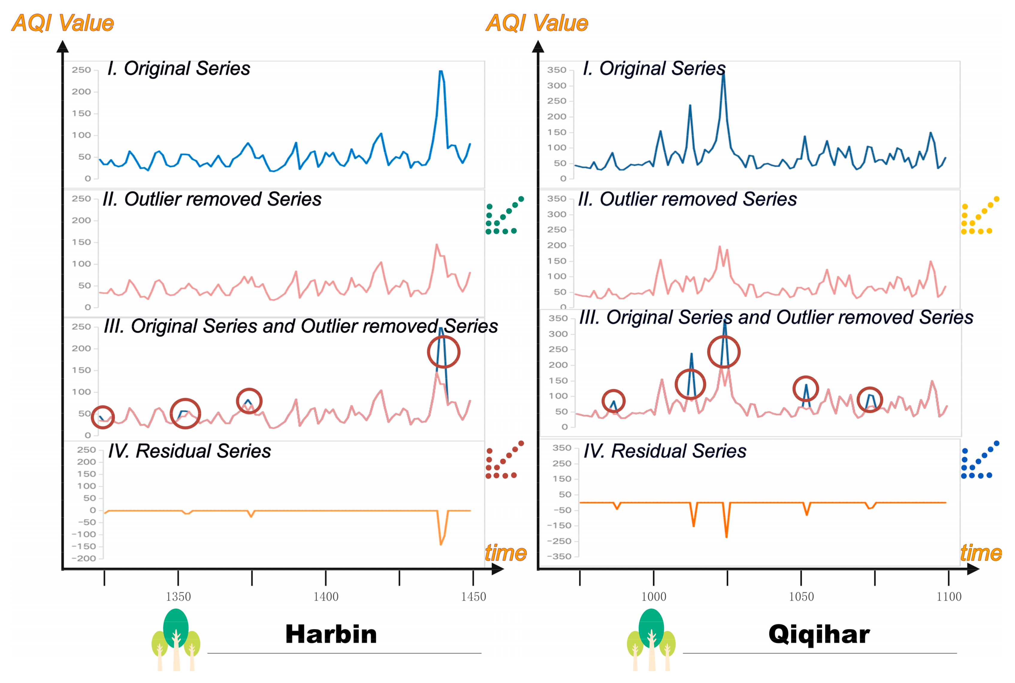
3.2. Data Preprocessing
For the missing value of AQI in raw data, cubic line interpolation was utilized to fill in that. Cubic spline interpolation is widely used in numerical analysis and computer graphics to avoid data oscillations that can be caused by low-order interpolation by applying a smooth and microscopic cubic polynomial to the fit.
As for the outliers owing to the mutation of the air pollution series, the Hampel Filter method was implemented to detect the abnormal one and correct it. Its main principle can be summarized as follows: First, calculate the median of each group of data and the absolute deviation of each data point relative to the median. Then, judge the outliers through the threshold setting and replace them with the corresponding window median, to realize the correction of outliers.
In this paper, this subsection shows the results of data preprocessing as shown in
Figure 3. In this figure, the horizontal axis indicates the magnitude of the amount of time-series data, reflecting changes in time, while the vertical axis represents the different sequences and the size of the sequence values.
3.3. The Simulation Results of Forecasting Module
In this section, several comparative experiments were designed to test the performance of the proposed forecasting model under different scenarios. The evaluation matrixes introduced before were calculated to assess the forecasting accuracy.
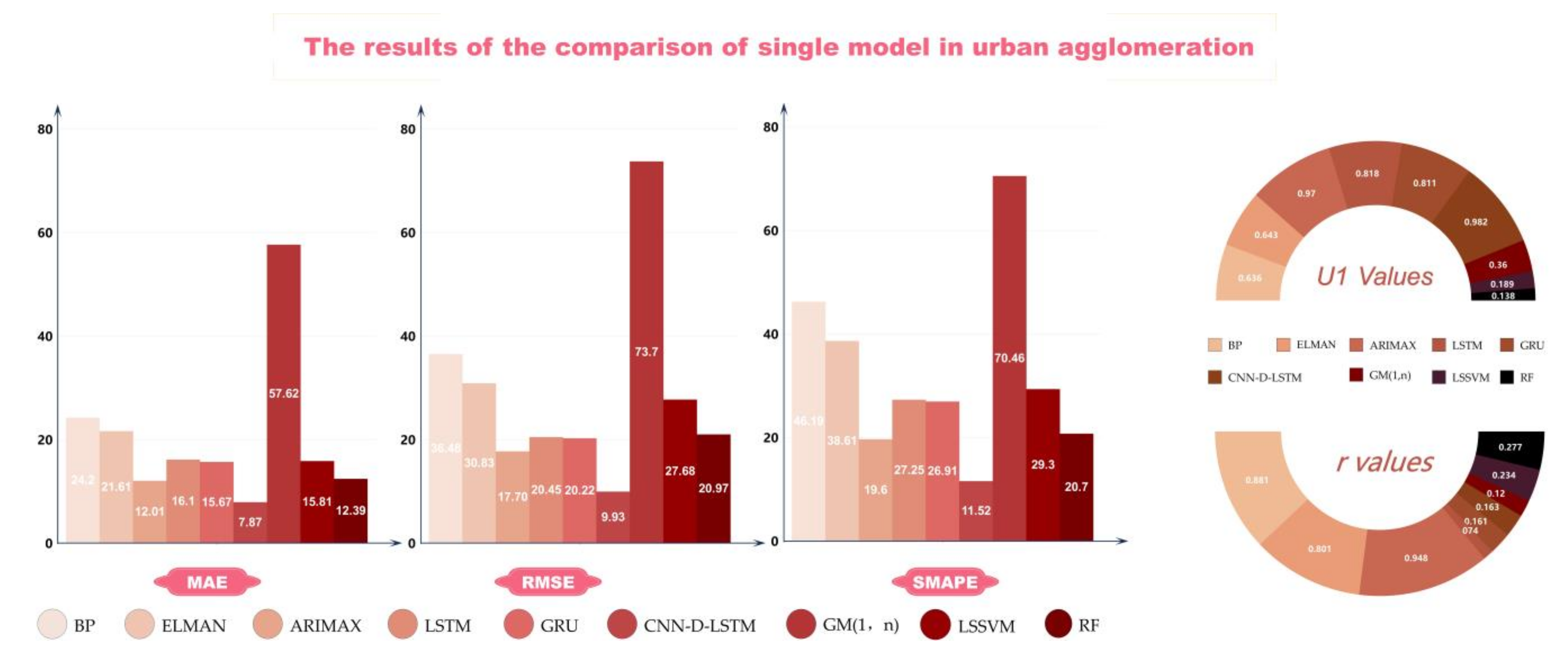
3.3.1. Compare of Single Model in Urban Agglomeration Forecasting
To demonstrate the superiority of our proposed single forecasting model in urban agglomerations, this subsection chose several traditional forecasting models representative of different types of forecasting methods. The comparative models contain Autoregressive Moving Average with Extra Input (ARIMAX), Grey Model (GM), Back Propagation Neural Network (BPNN), Elman Neural Network (ELMAN), Least Squares Support Vector Machine (LSSVM), Random Forest (RF), Long Short-Term Memory networks (LSTM), Gated Recurrent Unit networks (GRU) and our proposed model.
In this experiment, the data of whole cities were taken into forecasting, considering the general performance of the proposed model. Specifically, by the order of time, 70% of the collected data were divided into training sets, to make the model fit best; 30% of the data were treated as testing sets, to evaluate the forecasting performance of different models. The results of single model forecasting are shown in
Table 3, and the difference in performance can be seen in
Figure 4.
Analyzing the above results, conclusions could be made as follows:
(1) According to the results shown in
Table 3, from the comparison of different types of forecasting models, it is apparent that simple neural networks like the BP and ELMAN network, are not capable of accurately forecasting air quality in urban agglomerations.
(2) It is worth mentioning that the forecasting performance of ARIMAX was better than these two deep learning methods LSTM and GRU. Reflecting on the reasons for this phenomenon, it might be that ARIMAX performs well in the potential feature, which reveals the shortcomings of LSTM and GRU.
(3) Compared with other machine learning models, the superiority of CNN-D-LSTM could be identified, with lower error between actual values and predicted values. Moreover, the grey model seems to capture poor ability in forecasting air quality time series.
(4) For the former four evaluation indicators, our proposed model CNN-D-LSTM reached the smallest, respectively, 7.8692, 9.9289, 11.5215% and 0.0744. These indicators represent the improvement made by the proposed model and are more than two times compared with other models.
(5) For the correlation between the actual and forecasted value , that of the proposed model was close to 1, which reflects the superiority of its forecasting.
Remark 1: Generally, the performance and forecasting accuracy of the proposed model CNN-D-LSTM has gained significant improvement, in terms of the statistic. From these results, it seems to be accurate that our combined method of data preprocessing and the construct of DenseNet works well.
3.3.2. Compare the Performance on Different Clusters Divided
From the descriptive statistical analysis in
Table 2, conclusions could be made that different cities vary considerably in the characteristics of AQI changes. That means undifferentiated forecasting on an urban agglomeration, which takes the whole cities as a unit, is not desirable as disclosed in the above experiment. Conversely, if the clusters are divided appropriately based on the characteristics of AQI, the performance and accuracy of forecasting would be better.
Therefore, this subsection experiment was designed to confirm our assumption, by using different cluster division methods and varied indicators to measure the quality of division. This paper utilizes three different segmentation methods including k-mean clustering, hierarchical clustering and Gaussian hybrid clustering. In addition, three indicators were calculated, containing the Contour coefficient, Calinski–Harabasz Index (CH Index) and Davies–Bouldin Index (DB Index). The larger the Contour coefficient and CH Index are, the better clusters are divided, conversely, on the opposite.
In this experiment, to simplify the analysis of results, the number of clusters was set to
n = 3. The results of this comparative experiment are shown in
Table 4 and
Figure 5. In
Figure 5, the horizontal axis indicates the different predictive models or treatments, while the vertical axis indicates the magnitude of the relative values of the evaluation metrics to make better comparisons.
From the results shown in
Table 4, conclusions could be made as follows:
(1) Compared with the results shown in
Table 3 using the proposed model, it can be asserted that different methods used in cluster division did affect the accuracy of forecasting in urban agglomeration. Taking each individual cluster, for example, as the clustering method changes the performance of forecasting varies.
(2) As the evaluation indicators show, the influence of clustering methods on the spatial forecasting of air quality might manifest in different clusters, which means it is sometimes hard to identify the overall performance.
(3) However, through Gaussian hybrid clustering, the accuracy of forecasting was significantly better than the results divided by the other methods. That means there exists an optimal division of clusters to aid the air quality forecasting in urban agglomeration.
(4) The conclusion drawn by comparison is consistent with that represented by three indicators, showing that these could play a role in assessing the effectiveness of cluster division.
Remark 2: To sum up, this experiment reflects that the appropriate division of urban agglomeration is helpful for improving the effectiveness and performance of air quality forecasting. It provides a feasible solution to address such forecasting that is spatial related.
3.4. The Properties Analysis of Network
In this subsection, the air pollution in Harbin–Changchun urban agglomeration was connected to analysis utilizing social networks. By doing so, the dynamic correlations and the extent of correlations were demonstrated clearly.
Based on the fundamental methods and related properties introduced in
Section 2, the AQI-weighted correlation network was constructed in
Figure 6, in which each node and directed linkage were included. Moreover, in the process of visualization, the color of nodes is to differ in the degree of each city. In other words, the node of redcolor has a higher degree in this cluster, which reflects its importance. Conversely, the node of another color represents the opposite. In addition, different types of arrows represent different meanings: bi-directional arrows indicate synchronized interactions between two parties, and uni-directional arrows indicate unidirectional influences with a lag, in which arrow pointing represents the direction of influence.
Like the correlation network shown above, there are a lot of properties to be calculated.
Table 5 shows a number of metrics that reflect the degree to which the node is centered.
From the results shown in
Table 5, some conclusions could be made:
(1) In terms of the property Degree, the values of Harbin, Daqing and Qiqihar were verified far higher than those of other nodes, which means these three cities are positioned closer to the center of the agglomeration.
(2) The reason behind the higher Degree could originate from the construction of spatial networks. These three cities have a lot of arrows pointing to them, revealing that other cities have air pollution lag effects.
(3) Betweenness centrality is used to reflect the potential ability of a node to propagate, influence and control in the network. Based on this value, it is clear that Daqing and Qiqihar could affect the control of air pollution in this agglomeration.
Remark 3: Based on the above analysis, the ability of social network analysis to analyze pollution prevention in urban agglomerations is well demonstrated, which is a further use of predictive modeling. By utilizing it, the important nodes could be identified to play their roles.
4. Discussion
In this section, further experiments or analyses were conducted to explore the generalization ability of our proposed complex system, including the robustness test of the forecasting module, and the dynamic analysis of social networks.
4.1. The Dynamic Analysis of Social Network
With the change in time, the characteristics of air pollution urban agglomeration will also change, the use of social networks to analyze its different periods can reflect the development of its change rules and trends over a period of time. So, in this part, the comparative analysis of two different periods was conducted to explore the dynamic development of air pollution correlations in the urban agglomeration.
By comparing the previous air pollution spatial network correlations for two different time periods in this urban agglomeration, this section can analyze the trend of the air pollution urban agglomeration synergistic effect during this period. This trend is mainly reflected in the strengthening of linkages and the increasing role of the dominant city in them (Detailed description listed in
Section S2 in Supplementary File, taking 2015 and 2020 for example).
So, through the analysis of dynamic change, the government can use it to analyze the pattern of change, judge the development trend, and prepare for pollution prevention and control.
4.2. The Stability of the Proposed System
Despite the system’s outstanding performance in comparing the forecasting accuracy of models of the same type, it does not go far enough in choosing the subgroup delineation model for urban agglomeration prediction.
On the one hand, it is clearly unreasonable to specify the number of subgroups in real scenario applications. Therefore, the optimal choice of the number of subgroup divisions still needs to be strengthened, and intelligent algorithm optimization and cohesive subgroup division methods can be considered.
On the other hand, considering the complexity of the model, the constructed forecastingmodel was not subjected to sensitivity analysis in this paper. Therefore, it is worthwhile to explore the extent to which parameter changes affect the prediction performance and the kind of parameter that affects it the most.
4.3. Multistep Forecasting of Proposed System
In order to further test the stability of the constructed model and to demonstrate its significant ability in multi-stepforecasting, the following discussion is carried out. In this subsection, the same urban agglomeration was selected as the researcher’s object, and our proposed forecasting model was applied to the multistep forecasting of air quality in those cities. Generally, air quality forecasts are more representative within a week, thus the steps ahead were set to be 1 day, 3 days, 5 days and 7 days. The same evaluation indicators were utilized to assess the accuracy of forecasting.
Based on the implementation of multi-step forecasting (Detailed description listed in
Section S3 in Supplementary File), the application capability of the proposed model is further confirmed. From the experimental results, the short-term multi-step forecasting (including within one day and three days) can still control the model accuracy above 90%, but in the longer-term multi-step forecasting(more than five days and seven days), its accuracy decreases faster.
5. Conclusions
5.1. Main Conclusions
This paper focuses on the combination of air quality forecasting and social network analysis in urban agglomerations, and a comprehensive air quality forecasting system is constructed through text sentiment analysis, feature processing methods and the CNN-D-LSTM model. Through experimental simulation and results analysis, the main conclusions are as follows:
(1) By combining the feature processing methods of filtering algorithms, embedding algorithms and PCA, key features can be extracted more efficiently and information loss can be avoided.
(2) The proposed CNN-D-LSTM model improves forecasting performance compared to other models, proving the effectiveness of adding DenseNet.
(3) Text sentiment analysis helps to capture the relationship between public sentiment and air quality, and its introduction into forecasting models can improve its performance.
(4) Social network analysis helps to reveal the spatial and temporal correlation of air quality within urban agglomerations, providing support for dynamic monitoring and policy formulation.
5.2. Academic Significance
The study of air quality forecasting systems constructed in conjunction with social network analysis has several important academic applications:
(1) Accurate Real-time Air Quality Monitoring: this paper introduces an innovative perspective into air quality forecasting, which takes public emotions into account, thus improving the accuracy of forecasting. Moreover, a deep learning model with adequate feature preprocessing could aid the capture of potential features in AQI data.
(2) Analysis of the Spatial Distribution of Air Pollution: by analyzing air pollution studies using social networks and constructing a network of correlations between urban nodes, the dynamic changes and interactions of air pollution within urban agglomerations could be revealed. It would provide related departments with useful information on the tendency and regularity of air pollution with time passing.
(3) The combination of air quality forecasting and decision-making: this paper attempts to take air quality forecasting into the assistance of decision-making. On the one hand, once air quality is forecasted, social networks can be used to assist in pollution prevention and control; on the other hand, the analysis of air pollution in urban agglomerations can assist in improving the other.
In conclusion, the air pollution forecasting system is able to analyze air pollution spatial distribution and provide more accurate information for decision-makers to rely on.
5.3. Practical Application
In practice, the application significance of the hybrid spatial air quality forecasting system constructed contains the following aspects:
(1) Improving the effectiveness of control: the forecasting system can provide decision-makers with the trend of future air quality changes, enabling government departments to take measures in advance to reduce the risk of air pollution.
(2) Improving joint prevention and control: social network analysis can reveal the correlation of air quality between cities, which means key cities could be identified to help the joint prevention and control under limited labor and material resources.
(3) Promoting sustainable development: the forecasting system proposed in this paper can provide government departments with information about changes in air quality, which can help to fully consider the correlations in the planning process and realize the coordinated development of the economy, society and environment.
In conclusion, the air pollution forecasting system can improve the effectiveness of environmental management and promote the sustainable development of the ecological environment through joint prevention and control by government departments.
5.4. Future Research Directions
The following research directions will be explored in the future.
(1) Hyperparameter optimization: To consider what impact the different hyperparameters of proposed models would have, the future goal of forecasting studies in urban agglomeration is to use AutoML approaches, assisting in the selection of optimal models [
59,
60]. Sensitivity analysis would study to what extent the different hyperparameters would have an influence in the future.
(2) Policy evaluation and optimization: based on the forecasting model and real-time monitoring data, the effectiveness evaluation and optimization of air quality management policies can be further studied. By simulating the air quality changes under different policy scenarios, it provides a scientific basis for policymakers.
(3) Expanding application areas: in future research, the research methodology can be applied to other environmental problems such as water quality prediction and noise pollution prediction to support broader environmental management and governance.


