Article

Modeling and IAHA Solution for Task Scheduling Problem of Processing Crowdsourcing in the Context of Social Manufacturing

1
Key Laboratory of Advanced Manufacturing and Automation Technology, Education Department of Guangxi Zhuang Autonomous Region, Guilin University of Technology, Guilin 541006, China
2
College of Mechanical and Control Engineering, Guilin University of Technology, Guilin 541006, China
*
Author to whom correspondence should be addressed.
Systems 2023, 11(8), 383; https://doi.org/10.3390/systems11080383
Submission received: 12 June 2023 / Revised: 14 July 2023 / Accepted: 25 July 2023 / Published: 27 July 2023
(This article belongs to the Special Issue Manufacturing and Service Systems for Industry 4.0/5.0)

Abstract

:
The paper addresses the discrete characteristics of the processing crowdsourcing task scheduling problem in the context of social manufacturing, divides it into two subproblems of social manufacturing unit selecting and subtask sorting, establishes its mixed-integer programming with the objective of minimizing the maximum completion time, and proposes an improved artificial hummingbird algorithm (IAHA) for solving it. The IAHA uses initialization rules of global selection, local selection, and random selection to improve the quality of the initial population, the Levy flight to improve guided foraging and territorial foraging, the simplex search strategy to improve migration foraging to enhance the merit-seeking ability, and the greedy decoding method to improve the quality of the solution and reduce solution time. For the IAHA, orthogonal tests are designed to obtain the optimal combination of parameters, and comparative tests are made with variants of the AHA and other algorithms on the benchmark case and a simulated crowdsourcing case. The experimental results show that the IAHA can obtain superior solutions in many cases with economy and effectiveness.

1. Introduction

Social manufacturing [1,2,3] is based on the information-physical-social interconnection of social manufacturing resources (SMR), as well as the self-organization of social resources and collaborative interaction and information sharing. It is a future-oriented service-oriented manufacturing model that covers the deep participation of distributed producers and consumers in the whole life cycle of products. In the social manufacturing model, decentralized social manufacturing resources collaboratively perform multiple manufacturing tasks based on multiple interest coordination and social mechanisms; in other words, their processing tasks are distributed through crowdsourcing and performed by discrete social manufacturing resources. As a new SOM model, social manufacturing has the characteristics of small and microenterprises, social resources, interconnection and interaction, product personalization, organization decentralization, and distribution. Among them, decentralization is an important feature of social manufacturing that is different from other manufacturing modes. With the continuous enhancement of the flat self-organized dynamic manufacturing community, the core enterprise no longer has the dominant power in the manufacturing network, and the traditional seller’s market has gradually transferred to the buyer’s market [1,4]. The task scheduling of processing crowdsourcing is an important link in the social manufacturing mode. The core of the problem to be solved lies in the reasonable allocation of effective resources and the necessary optimization means. The purpose is to arrange the crowdsourcing tasks into SMRs in a reasonable and balanced way and to make a reasonable plan for the processing sequence of tasks on SMRs. Because task scheduling is a process with a complex environment and many uncertain factors, the quality of scheduling directly affects the competitiveness of social manufacturing resources involved in product manufacturing in the market. Therefore, an algorithm is needed for task scheduling and planning of SMR for collaborative manufacturing crowdsourcing tasks. In this context, the problem of processing crowdsourcing task scheduling in socialized manufacturing is proposed.
In general, except for manufacturing units that are socially dispersed, the processing crowdsourcing task scheduling problem in communalized manufacturing can usually be classified as the flexible job shop scheduling problem (FJSP) [5], and the FJSP problem has been proven to be an NP-hard problem [6]. For this difficult problem, experts and scholars have conducted decades of research and proposed many methods to solve it. Among them, the classical methods include the Lagrangian relaxation algorithm [7], dynamic programming [8], and branch-and-bound algorithm [9]; however, these classical solution methods have more or less some restrictions, such as requiring the function to be derivable, or convex, or the solution size cannot be too large, which restrict their applications. To overcome these shortcomings, scholars have developed heuristic algorithms, such as genetic algorithms [10,11], differential evolutionary algorithms [12], ant colony algorithms [13], particle swarm algorithms [14,15,16], artificial bee colony algorithms [17], and other intelligent optimization algorithms; however, traditional heuristic algorithms often have the disadvantages of slow running speed and easy to fall into local optimality in the late iteration. To address these drawbacks, experts and scholars at home and abroad have proposed many improvements in using them to solve FJSP, e.g., Wang et al. [18] designed three heuristic strategies and proposed a new artificial bee colony algorithm HMABC to achieve scheduling of practical production activities; Yuan et al. [19] developed a new transformation mechanism to enable differential evolutionary algorithms on continuous domains to explore discrete FJP problems; Sun et al. [20] proposed a method for combining crossover and variational operators considering machine load balancing and designed an improved hybrid genetic algorithm HGA-VNS for local search of critical processes on critical paths.
Currently, the research for FJSP is mainly in considering novel conditions such as uncertainties and green low-carbon requirements and constructing novel solution algorithms such as multiobjective intelligent optimization and deep learning. For example, Xu et al. [21] proposed a load-balancing-based step-size adaptive discrete particle swarm algorithm (LS-DPSO) to solve the G-FSP model. Wang et al. [22] considered the maximum completion time, total delay time, and total energy consumption of the job and used the hybrid adaptive differential evolution algorithm (HADE) to solve it. Lou et al. [23] combined adaptive local search and a multiobjective evolutionary algorithm and proposed a multiobjective modal algorithm based on learning decomposition (MOMA-LD) to solve the model. Yan et al. [24] studied the FJP problem with the objectives of maximum completion time, total workload, critical machine workload, and minimum advance/delay penalties and proposed an improved ant colony algorithm to solve the problem. Tian et al. [25] established an algorithm with the objectives of work duration, total machine load, machine on/off times, and tool change times as the objectives of a multiobjective optimization model and solved the model using NSGA-II.
Although more research has been conducted for FJSP, it has mainly focused on scheduling production lines within a single plant. Due to the similarity of work conditions, it has gradually been applied in recent years in areas such as aerospace materials manufacturing [18] and distributed factory production scheduling [26], while further research is needed in processing crowdsourcing task scheduling. The objective of this study is to develop a mixed-integer programming model for scheduling processing crowdsourcing tasks in community-based manufacturing and to design algorithms to solve it in order to improve the productivity of processing crowdsourcing tasks. In this task scheduling optimization problem, one or more SMRs with the ability to provide specialized manufacturing services externally are regarded as social manufacturing units (SMU), which are characterized by socialization, decentralization, and specialization. SMRs may come from traditional large- and medium-sized enterprises that decompose and reorganize their internal manufacturing resources into several small and microenterprises with independent manufacturing service capabilities or from emerging small and microenterprises in market segments, start-up companies, or individuals with professional skills [3]. Each individual crowdsourced task will be coordinated by multiple decentralized SMUs to produce a complex product. For this purpose, the manufacturing task of the product is decomposed, and the manufacturing of a collection of parts or components in the product is defined as tasks, and the collection of manufacturing operations of parts or components is defined as subtasks. The manufacturing of a product can be decomposed into multiple tasks, and each task can be further decomposed into more subtasks; each subtask can be processed by multiple SMUs, and all subtasks of the same task have a serial order constraint relationship with each other. Then, all subtasks are matched with SMUs according to the optimization objective to get the optimal scheduling scheme. Figure 1 shows a conceptual model for processing crowdsourced task scheduling in social manufacturing.
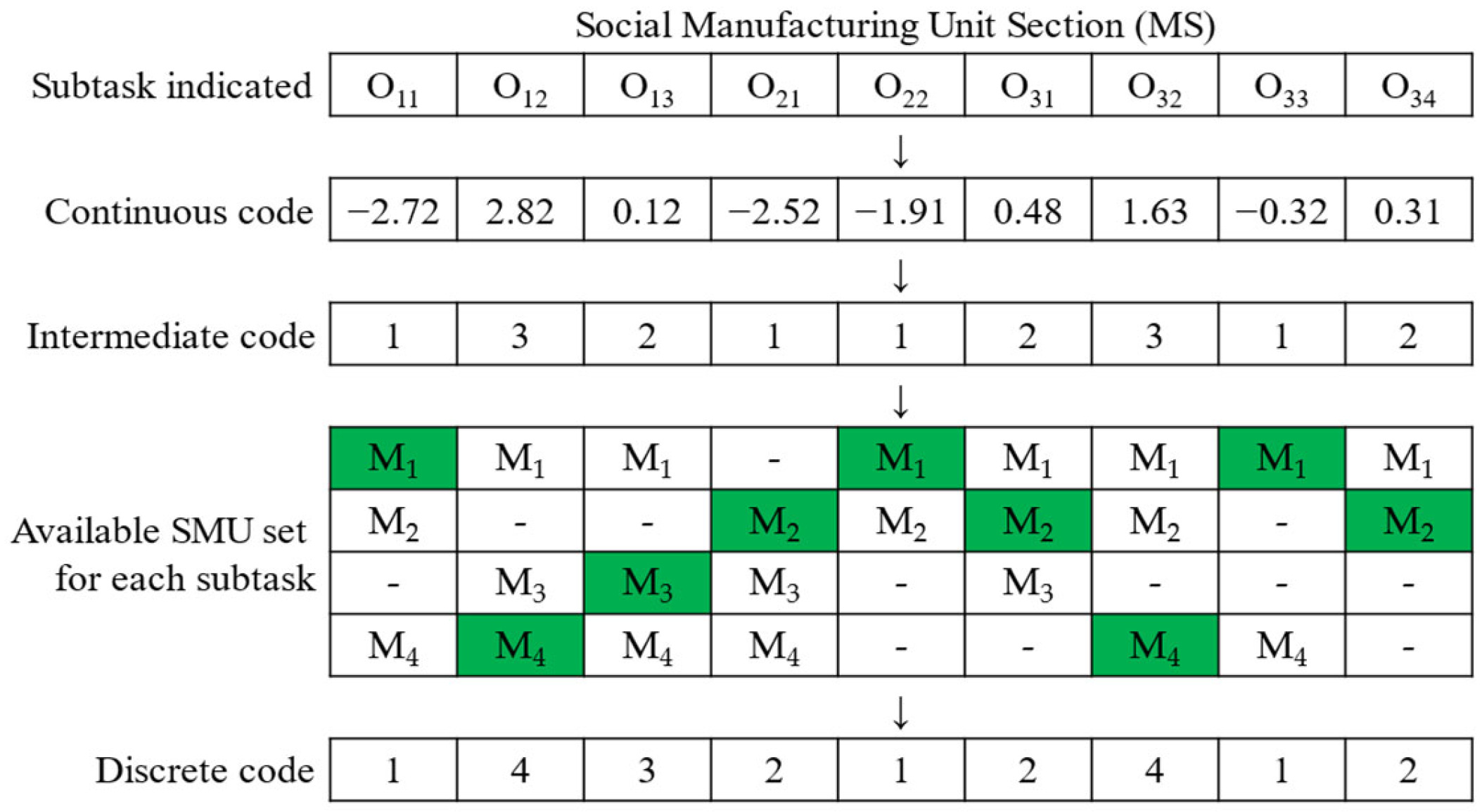
This study addresses the scheduling problem of processing crowdsourcing tasks in socialized manufacturing, establishes a mathematical model of scheduling with the objective of minimizing the maximum completion time, and proposes an improved artificial hummingbird algorithm (IAHA) to solve it. For its discrete characteristics, we divide the problem into two subproblems—social manufacturing unit selection and subtask sequence—and encode them separately according to the subproblem characteristics, match different decoding for the two encodings, and use greedy decoding methods to improve the quality of the solution. To improve the quality of the initial population of the IAHA, we used the initialization rules of global selection, local selection, and random selection (GLR). To enhance the merit-seeking ability of the IAHA, we used the Levy flight to improve the guided foraging and territorial foraging of the IAHA and the simplex search strategy (SSS) to improve the migration foraging of the IAHA. We designed four experiments, and the experiment results proved the superiority and effectiveness of the IAHA.
The rest of the paper is organized as follows: Section 2 defines the processing crowdsourcing task scheduling problem in social manufacturing and develops a mathematical model of the problem. Section 3 illustrates the IAHA in detail with a problem case. Section 4 conducts four experiments and discusses the results of the IAHA’s experiments on the benchmark and crowdsourcing case. Section 5 summarizes the main contents of the paper and points out future research directions.

2. Problem Modeling

2.1. Problem Definition

The processing crowdsourcing task scheduling problem in social manufacturing can usually be described as follows: n tasks are processed in m SMUs, each involving multiple subtasks; each subtask can be processed on multiple SMUs, and the processing time varies from SMU to SMU. In this study, the scheduling problem is divided into two subproblems: determining the processing SMUs for each subtask and determining the processing sequence on each SMU. Each subtask is assigned to the appropriate SMU, and the order in which subtasks are assigned to each SMU is determined.

2.2. Constraints

Before building the mixed integer programming model, some constraints need to be satisfied: (1) only one subtask can be processed by the same SMU at the same moment; (2) the same subtask of the same task can be processed by only one SMU at the same moment; (3) each subtask of each task cannot be interrupted once it starts processing; (4) different tasks have the same priority among themselves; (5) the subtasks of different tasks have no sequential constraints between the different tasks and sequential constraints between subtasks of the same workpiece; (6) all tasks can be machined at zero moments; (7) each subtask has the same processing effect on all SMUs that satisfy its processing conditions; (8) the transport time when moving subtasks between SMUs is ignored; (9) the processing time of each subtask and its optional set of processing SMUs are known.

2.3. Mathematical Models

Some symbols need to be defined before the mathematical model can be built, and Table 1 shows some of the symbols that appear in FJSP and their corresponding meanings.
In solving the scheduling problem of crowdsourcing tasks in community-based manufacturing, the maximum completion time is chosen as the evaluation index to measure the merits of the scheduling scheme. The completion time is the time when the last process of each workpiece is completed, the latest of which is the maximum completion time, which is the most fundamental indicator of the scheduling scheme, mainly reflecting the productivity of the shop floor, and is the most widely used evaluation indicator in the study. It can be expressed as follows:
f = m i n ( m a x ( C j ) ) ,   1 j n
The problem is subject to the following constraints:
S j h + x x j h × p i j h     C j h ,   i = 1 , 2 , , m ;   j = 1 , 2 , , n ;   h = 1 , 2 , , h j
  C j h S j ( h + 1 ) , j = 1 , 2 , , n ;   h = 1 , 2 , , h j 1
C j h j C max ,   j = 1 , 2 , , n
S j h + p i j h S k l + L 1 y i j h k l ,   j = 0 , 1 , 2 , 3 , , n ; k = 1 , 2 , , n ;   h = 1 , 2 , , h j ; l = 1 , 2 , , h k ;   i = 1 , 2 , , m
C j h S j ( h + 1 ) + L 1 y i k l j ( h + 1 ) ,   j = 1 , 2 , , n ; k = 0 , 1 , 2 , , n ;   h = 1 , 2 , , h j 1 ; l = 1 , 2 , , h k ;   i = 1 , 2 , , m
i = 1 m j h x i j h = 1 ;   h = 1 , 2 , , h j ;   j = 1 , 2 , , n
S j h 0 ,   C j h 0 ,   j = 0 , 1 , , n ;   h = 1 , 2 , , h i
(2) and (3) denote the sequential order constraint of the subtasks of each task; (4) denotes that the completion time of a single subtask is less than the total completion time; (5) and (6) denote that the same SMUs cannot process multiple subtasks at a certain time; (7) denotes the SMU constraint that there cannot be more than one SMU processing the same process at a certain time; (8) denotes that each parameter variable is positive.

3. Improved Artificial Hummingbird Algorithm for Model Solving

The artificial hummingbird algorithm (AHA) is a novel metaheuristic algorithm proposed by ZHAO et al. [27] in 2021. The AHA is inspired by the special flight skills and intelligent foraging strategies of hummingbirds. The AHA has been applied in the distributed power optimization configuration [28], coordinated scenery-thermal power generation scheduling [29], and arrhythmia classification [30]. We try to apply it to solve the processing crowdsourcing task scheduling model in social manufacturing and combine the characteristics of the crowdsourced task scheduling model to modify the AHA and refer to the improved artificial hummingbird algorithm as the IAHA, which is described in detail in this section.

3.1. Discrete Transformation

The AHA, as a new type of swarm intelligence optimization algorithm, has the advantages of few parameters, strong search capability, and easy implementation [27], but it also has the common problems of swarm intelligence optimization algorithms, such as slow convergence speed and easy to fall into local optimum [31]. In response to these drawbacks and the discrete characteristics of the processing crowdsourcing task scheduling problem, an improved artificial hummingbird algorithm (IAHA) is proposed in the study. To describe the problem more clearly, we introduce an example to illustrate it, and the processing information for each task is shown in Table 2.

3.1.1. Question Encoding

The crowdsourcing task scheduling problem contains 2 components: social manufacturing unit selection (MS) and subtask sequencing (SS). We use a two-segment encoding based on SMU and subtasks, respectively, and the length of both encodings is the total number of subtasks T0. The range of values for each value on the encoding is [−δ, δ]. If δ is obtained too small, the relative size of the updated individual subtask sequence value changes a lot, leading to the destruction of individuals; if δ is obtained too large, it will lead to an insignificant Levy flight effect, which is generally set to a number between 2 and 5. A legal encoding is shown in Figure 2.

3.1.2. Code Transformation

The solution space of the AHA is a continuous space, and the processing crowdsourcing scheduling problem is a discrete combinatorial optimization problem, which requires mapping the continuous solution space to a discrete solution space. Different transformation mechanisms are required due to the different constraints on SMU selection and subtask sequence.
(1)
MS section
The continuous codes are converted into discrete codes according to Equation (9) and then converted into specific SMU numbers according to the subtask optional SMUs. When only one SMU of subtask Ojh is processable, the discrete encoding value is taken as 1. In the MS, the SMU corresponding to each subtask of each task is shown from left to right.
u i = 1 i f   m j h = 1 r o u n d e i + δ m j h 1 2 δ + 1 e l s e ,   i = 1 , 2 , , d 2
where is e(i) the i-th value of the MS continuous code; mjh is the number of processing SMUs available for subtask Ojh; u(i) is the i-th value of the transformed MS discrete code.
Figure 3 shows an MS transformation, where “-” indicates that the SMU is not available, the value of the intermediate code “i” indicates that the i-th SMU is selected for processing among the available SMUs of the subtask, and the value of the discrete code indicates the SMU selected for the subtask. For example, the intermediate code “3” of O12 means that the third SMU (M4) is selected from the set of available SMUs {M1, M3, M4} of O12, and the discrete code of O12 is 4. For the SMU selection problem, the above code and its conversion method do not generate illegal solutions.
(2)
SS section
The largest position value (LPV) rule [19] is used to transform the solution space of the subtask sequence. The values on the SS are assigned a fixed ID starting from 1. Then, they are sorted in order from largest to smallest. Finally, a new code is obtained based on the fixed ID corresponding to each value, which is converted into a sequence that can be used for decoding according to the number of subtasks of each task.
Figure 4 shows a SS transformation where the 9 in fixed ID maps both continuous code 1.31 and task J3, and after LPV sort, the 9 moves to the 5th bit of the code. The value in the discrete code indicates the task number, and the number of occurrences of “i” from left to right indicates the i-th subtask of the task. At this time, the 5th bit of the discrete code is mapped to 3, indicating task J3, and 3 is the 2nd occurrence, and O32 is in the 5th position of the processing. Figure 4 indicates the processing order of O31 → O21 → O22 → O11 → O32 → O12 → O13 → O33 → O34.

3.1.3. Problem Decoding

The encoding of the crowdsourced task scheduling problem consists of two parts, MS and SS, which need to be decoded separately. The decoding steps are as follows:
(1)
MS section
The MS is read from left to right and converted into SMU order matrix JM and time order matrix T, where JM(j, h) denotes the SMU number of subtask Ojh; T(j, h) denotes the processing time of subtask Ojh. Take the code of Figure 3 as an example, combined with processing information in Table 2, and MS is converted to JM and T as follows:
J M = 1 4 3 - 2 1 - - 2 4 1 2
T = 2 2 4 - 3 5 - - 3 8 6 4
(2)
SS section
The SS is read sequentially from left to right, and the greedy decoding method (GDM) is used to find the free time of each SMU and decide whether to insert subtasks into the free time according to Equations (12) and (13). In this way, until all subtasks on the sequence are scheduled in their optimal positions, obtaining a higher quality scheduling scheme.
M S j h = max C j h 1 , I T S k
S j h = M S j h i f   M S j h , M S j h + P i j h I T S k , I T E k max C j h 1 , L M e l s e
where MSjh denotes the start processing time of subtask Ojh satisfying the insertion condition; Cj(h−1) denotes the processing completion time of subtask Oj(h−1); ITSk, ITEk denotes the start time and end time of the k-th idle time period, respectively; LM denotes the end time of the last current subtask of the SMU selected by the subtask; Sjh denotes the start processing time of subtask Ojh. If the insertion condition [MSjh, MSjh + Pijh] ⊆ [ITSk, ITEk] is satisfied, then Sjh = MSjh.
Figure 5 shows a GDM operation where O22 was originally machined in M1 after O32. There is a long idle time between O11 and O32. At this time, the possible start time of O22 MS22 = max (5, 5) = 5, the processing time P122 = 4, the 1st idle time period [ITS1, ITE1] = [5, 11], and the insertion condition [5, 9] ⊆ [5, 11] are satisfied, so that the completion time can be shortened.

3.2. Population Initialization

Population initialization is a key problem in evolutionary algorithms, and the quality of the initial solution has a great impact on the speed and quality of the algorithm’s solution. The AHA performs random initialization of the initial population, which cannot guarantee the quality of the initial solution, so we use the GLR method for population initialization, including global selection, local selection, and random selection [32]. GS considers the global load balance of all SMUs. LS only considers the global SMU load balance during each task processing. GS and LS make the workload of each selected SMU as balanced as possible to fully improve the utilization of SMUs. RS mainly considers distributing the initial population as decentralized as possible throughout the solution space to improve the diversity of solutions. The three methods account for a population ratio of GS:LS:RS = 0.4:0.4:0.2, and the quality of the initial solution is improved by the combination of the three methods. The initialized population encoding is discrete and needs to be inverse transformed to continuous encoding according to Section 3.1.2 in order to use the IAHA for searching.

3.3. Levy Flight

The Levy flight is a random search path that obeys the Levy distribution [33]. Since the Levy distribution is a heavy-tailed distribution, the Levy flight is a search method with short and occasionally long-distance intervals. Currently, the Levy flight is widely used in intelligent optimization; for example, Liu et al. [34] used the levy flight combined with a differential evolution algorithm to solve the JSP problem. We introduced the Levy flight in the guided foraging and territorial foraging of the IAHA to enhance its search capability and ability to jump out of the local optimum.
After combining Levy flights, guided foraging and territorial foraging locations were updated as follows.
x i t + 1 = x i t + α L e v y λ f x i t f v i t + 1 v i t + 1 f x i t f v i t + 1
where xi (t) is the t-th generation position of xi; ⊕ is the point multiplication; α is the step control factor; vi (t + 1) is the location of the candidate food source obtained by the AHA through guided foraging osr territorial foraging [27]; Levy(λ) is the random search path, calculated as follows:
L e v y λ = s λ ,   1 < λ 3
where the step size s is calculated as follows:
s = μ v 1 / β
where β is taken as a constant 1.5, and µ and v follow normal distribution defined as follows:
μ N 0 ,   σ μ 2 ,   v N 0 ,   1
where
σ μ = Γ 1 + β sin π β 2 Γ 1 + β 2 β × 2 β 1 2 1 β

3.4. Simplex Search Strategy

The simplex search strategy (SSS) uses iterative local search [35] to improve the migration foraging of hummingbird flocks in the IAHA. The centroid location of the hummingbird xc(t) at the t-th iteration is calculated as follows.
x c t = 1 N i = 1 N x i t
The position of the worst hummingbird is mapped around centroid xc(t) to obtain the mapped position xr(t), which is calculated as follows:
x r t = 2 x c t x w o r t ,
where wor is the index of the worst-performing hummingbird.
The fitness of the mapped position xr(t) guides the search of the search space. The new position of the worst-performing hummingbird xwor(t + 1) is obtained by comparing the fitness of the mapped position xr(t), the optimal position xbest(t) and the second worst position xswor(t), calculated as follows:
x w o r t + 1 = 1 + γ x c t γ x w o r t f x r < f x b e s t x r t f x b e s t < f x r < f x s w o r 1 β x c t + β x w o r t f x r > f x s w o r
where γ is the expansion factor; β is the contraction factor.
The IAHA can be obtained by combining the above-mentioned improved methods for the AHA, and its flow chart is shown in Figure 6.

4. Experimental Results and Discussion

Four sets of experiments are conducted in the section: (1) designing orthogonal experiments to configure the optimal combination of parameters for the IAHA; (2) discussing the performance improvement of the improved strategy of the IAHA over the AHA and its variants; (3) comparing the performance with algorithms proposed by other scholars in a standard algorithm; (4) simulating a real processing crowdsourcing environment for scheduling. And the first three sets of experiments are checked for significant differences in the experimental results by the Friedman test [36]. At present, there is no public crowdsourcing task data set in the research of social manufacturing, so this paper adopts Kacem [37] and Brandimarte [38] standard cases, which are commonly used in FJSP, in the first three experiments. Kacem and Brandimarte belong to total FJSP(T-FJSP) and partial FJSP(P-FJSP), respectively. The expression of T-FJSP and P-FJSP in this paper is that subtasks can be processed on any SMU, and subtasks can only be processed on some SMU, respectively. T-FJSP belongs to the P-FJSP category.
The hardware environment for the simulation experiments in the study is Intel(R) Core (TM) i5-10400 CPU @ 2.90 GHz; RAM 16 GB; software environment is Windows 10, written in Python, simulation platform PyCharm 2020.1.

4.1. Comparison of Orthogonal Experiments of Parameters

The size of the parameters has a large impact on the performance of the IAHA. Therefore, we need a reasonable configuration. The main parameters of the IAHA are shown in Table 3.
In the IAHA, r1, r2, and r3 determine the choice of flight skill each time foraging is performed, and the sum of the three parameters is one, which can actually be considered as two parameters. f1 and f2 determine the foraging mode chosen each time, and the sum of f1 and f2 is 1, which can be considered as one parameter. The IAHA only performs migration foraging once every m iteration, so the influence of γ and β in SSS on the IAHA’s foraging performance is low, and in order to balance the convergence speed of SSS with the foraging performance, γ = 2 and β = 0.5 are often taken. Finally, there are five important parameters that have a great influence on the performance of the IAHA, which are δ, r1, r2, f1, and m.
We designed orthogonal experiments to configure the best parameter combinations, and the above five parameters are set as five factors with four levels for each factor. According to the principle of orthogonal experimental design, only 16(42 = 16) sets of parameter combinations need to be tested to find the best parameter configuration. The orthogonal test table L16(45) is shown in Table 4.
In the orthogonal experiments, the number of iterations of the algorithm is 200, and the population size is 200. Five cases of the standard test case Kacem [37] are used for the experiments to adjust the parameters, and 10 experiments are conducted for each case to take the average value as the experimental results; Table 5 shows the experimental results of the orthogonal experiments.
Friedman’s ranking of the experimental results was performed, and the sum of the result ranking of each experimental scheme in each case was calculated to obtain the final ranking of the schemes. The ranking and final ranking of each experimental scheme are shown in Table 6, which shows that the final ranking of experiment 10 is better than the other experimental schemes.
Significance tests were performed on the ranking results of this orthogonal test scheme. The original hypothesis H0: there are no significant differences in the results of the orthogonal experiment. The alternative hypothesis H1: there are significant differences in the results of the orthogonal experiment.
The results of the Friedman statistics of the program are shown in Table 7. From Table 7, the Friedman statistic is χ2 = 46.17, and the degree of freedom is k-1 = 15. When the significance level α is 0.05, querying the chi-square distribution table yields χ 0.05 ( 15 ) 2 = 25. Since χ2 > χ 0.05 ( 15 ) 2 , H0 is rejected, and H1 is accepted: there are significant differences in the results of the orthogonal experiment. When the significance level α is 0.01, the chi-square distribution table χ 0.01 ( 15 ) 2 = 30.58. Since χ2 > χ 0.01 ( 15 ) 2 , H0 is rejected, and H1 is accepted: there are significant differences in the results of the orthogonal experiment.
In summary, the results of the Friedman test with two significance levels of 0.05 and 0.01, in turn, showed that there are significant differences in the results obtained from this orthogonal test scheme, and the best performance was achieved with the parameter combination of test 10. Therefore, the parameter combination in test 10 was used as the algorithm parameter values for the IAHA in the later experiments with δ = 4, r1 = 0.27, r2 = 0.30, f1 = 0.55, and m = 10.

4.2. Comparison of IAHA and Other Variants of AHA

To verify the effects of the improvements made on the performance of the IAHA, variants of the AHA were constructed for comparison experiments, as shown in Table 8. Four improvement strategies were used to improve the AHA in three aspects where the GDM is an improvement of the decoding method, GLR is the initialization of the population using GLR, and the Levy flight and SSS are improvements of the foraging method for hummingbirds.
In the comparison experiments, the number of iterations of all algorithms is 500, and the population size is 300. Five cases of the standard case Kacem are used for experiments to compare the effect of the improved method on the performance of the algorithm. Ten experiments are conducted for each case, and the mean square error (MSE) is calculated by Equation (22) and used as the experimental results along with the mean (Mean), as shown in Table 9.
M S E = 1 n i = 1 n r i r min 2
where n = 10; ri is the maximum completion time obtained for each experiment; rmin is the optimal value of the maximum completion time known to be studied for each case, The rmin of Kacem 1–5 [37] are 11, 14, 11, 7, and 11, respectively [38].
According to the experimental results, the AHA deviates from other algorithms in Mean and has difficulty in searching rmin due to its relatively simple foraging method, which leads to its poor performance on MSE. The AHA-Levy-SSS improves the foraging method, the global and local search ability of the algorithm is enhanced, and, finally, outperforms the AHA on MSE. The AHA-GDM and AHA-GLR optimized the decoding method and initial population; the performance was slightly better than the AHA but still inferior to the AHA-Levy-SSS due to its relatively poor foraging ability. The IAHA achieved the best performance on both Mean and MSE.
Friedman’s ranking was performed based on the Mean of the experimental results, and the sum of the result ranking of each algorithm in each case was calculated to derive the final ranking of the scheme. The ranking and final ranking of each algorithm are shown in Table 10.
Significance tests were performed on the ranking results of five algorithms. The original hypothesis H0: there are no significant differences in the performance of each algorithm. The alternative hypothesis H1: there are significant differences in the performance of each algorithm.
The results of Friedman’s statistics for the comparison experiments are shown in Table 11. From Table 11, the Friedman statistic is χ2 = 18.64, and the degree of freedom is k − 1 = 4. When the significance level α is 0.05, querying the chi-square distribution table yields χ 0.05 ( 4 ) 2 = 9.49. Since χ2 > χ 0.05 ( 4 ) 2 , H0 is rejected, and H1 is accepted: there are significant differences in the performance of each algorithm. When the significance level α is 0.01, the chi-square distribution table χ 0.01 ( 4 ) 2 = 13.28. Since χ2 > χ 0.01 ( 4 ) 2 , H0 is rejected, and H1 is accepted: there are significant differences in the performance of each algorithm.
To observe the specific performance of the algorithms during iterations, Figure 7 plots the convergence curves of the maximum completion time (makespan) with the number of iterations for the five algorithms in one iteration of Kacem case 5. The populations diverge at the first generation of individuals. The IAHA and AHA-GLR with GLR showed excellent makespan, demonstrating that GLR significantly improved the quality of the initial populations. As iterations increase, the AHA-Levy-SSS, with its excellent search capability, quickly closes the gap with the AHA and AHA-GDM and surpasses the AHA-GLR after 50 iterations, proving that Levy and SSS enhance the search capability of the AHA and accelerate the convergence speed. Although the AHA-GDM is inferior to the AHA-GLR and AHA-Levy-SSS, it is always ahead of the AHA throughout the iterations, and the AHA-Levy-SSS, which lacks the GDM, always lags behind the IAHA at iteration number 100–200 due to the lack of GDM’s ability to optimize the scheduling results, proving that the GDM has the ability to optimize the scheduling results.
In summary, the results of the Friedman test with two significance levels of 0.05 and 0.01 show that the results obtained by the five algorithms are significantly different, and the IAHA achieves the best performance. The four strategies play major roles in different stages of the IAHA. In the early IAHA, the prepopulation quality is optimized mainly by GLR so that the IAHA can find relatively good scheduling results without too many iterations; in the middle IAHA iteration, the optimization-seeking ability of the algorithm is enhanced mainly by Levy and SSS to make it converge quickly; in the late IAHA iteration, the quality of scheduling results is improved mainly by the GDM.

4.3. Comparison of IAHA and Other Algorithms

To verify the effectiveness and superiority of the IAHA in solving crowdsourced task scheduling problems, the first 10 cases from the standard Brandimarte case [38] and 5 cases from Kacem [37], which are more commonly studied, are selected for experiments. The IAHA adjusts the population size and the number of iterations appropriately according to the case size, and the adjustment results are shown in Table 12, where n is the number of tasks and m is the SMU number.
The IAHA was run five times independently on each case to take the optimal solution, and the experimental results were compared with other algorithms, as in Table 13, where C* indicates the optimal value of makespan currently searched for that case in the literature and the optimal solution searched for by each of the Cmax algorithms, and “-” indicates that the algorithm did not provide data for that arithmetic case. The comparison algorithms are HA by Ziaee [39], PHMH by Bozejko [40], NIMASS by Xiong [41], ADCSO by Jiang [42], HLO-PSO by Ding [43], SLGA by Chen [44], and IAHA by the paper, where the experimental results of the comparison algorithms are from the original data in the literature.
Figure 8 shows the Gantt chart of the scheduling results obtained by the IAHA on the Mk10 case, respectively. In Figure 8, the first number on the block represents the task number, and the second number represents the subtask number
Since the IAHA searches for C* in all five Kacem cases and many algorithms do not provide results, the comparison between the IAHA and other algorithms will not be discussed later.
To facilitate a visual comparison of the performance of the IAHA with other algorithms on the Brandimarte cases, the experimental results are converted into relative percentage deviation (RPD). RPD is the percentage deviation of the algorithm result with respect to C*, which denotes the closeness of Cmax to C*, and is calculated as follows:
R P D = C max C * C * × 100 %
Table 14 shows the RPD results of the seven algorithms on the test cases. The average RPD of the IAHA achieves the smallest value, which indicates that the IAHA performs the best among the seven algorithms, especially on the Mk6 and Mk10 cases. The performance of the IAHA pulls away from the other algorithms by a large gap.
Friedman’s ranking was performed on the RPD, and the sum of the resultant rankings of each algorithm was calculated for each case to obtain the final ranking of the solutions. The ranking and final ranking of each experimental scheme are shown in Table 15, which shows that the final Friedman ranking of the IAHA is the best among the seven algorithms.
Significance tests were performed on the ranking results of seven algorithms. The original hypothesis H0: there are no significant differences in the performance of each algorithm. The alternative hypothesis H1: there are significant differences in the performance of each algorithm.
The results of Friedman’s statistics for the comparison experiments are shown in Table 16. From Table 16, the Friedman statistic is χ2 = 26.76, and the degree of freedom is k − 1 = 6. When the significance level α is 0.05, querying the chi-square distribution table yields χ 0.05 ( 6 ) 2 = 12.59. Since χ2 > χ 0.05 ( 6 ) 2 , H0 is rejected, and H1 is accepted: there are significant differences in the performance of each algorithm. When the significance level α is 0.01, the chi-square distribution table χ 0.01 ( 6 ) 2 = 16.81. Since χ2 > χ 0.01 ( 6 ) 2 , H0 is rejected, and H1 is accepted: there are significant differences in the performance of each algorithm.
In summary, the results of Friedman’s test with two significance levels of 0.05 and 0.01, respectively, show that there are significant differences in the performance of HA, PHMH, NIMASS, ADCSO, HLO-PSO, SLGA, and IAHA, and the IAHA has the best performance.

4.4. Application to Processing Crowdsourcing Task Scheduling

In order to further verify the effectiveness of the model and algorithm in this paper, we used 30 local small- and medium-sized manufacturing enterprises as SMUs, set the processing time of subtasks according to the enterprise scale, and simulated 15 processing crowdsourcing task data as cases. The processing crowdsourcing task case size is 15 × 30. The AHA and IAHA were used to simulate and solve them, respectively, and the parameter settings follow the results of the 4.1 orthogonal test; the number of populations is 300, and the number of iterations is 500.
The convergence curves can be obtained using the IAHA and AHA for the above case, as shown in Figure 9. It can be seen that the makespan of the IAHA and AHA converge at 105 and 116, respectively. The IAHA obtains a significantly better solution than the AHA and has a better performance in this processing crowdsourcing case. The IAHA, due to its unique initialization method, is already significantly in the lead in the early iterations of the algorithm and plays a key role in guiding the evolutionary direction of the population. In the late iteration of the algorithm, the IAHA is more likely to obtain better solutions due to its superior foraging method improvement strategy. Figure 10 shows the Gantt chart of the scheduling solution obtained by the IAHA.

5. Conclusions

In the social manufacturing model, dispersed manufacturing resources accomplish multiple manufacturing tasks collaboratively under multiple interest coordination and social mechanisms. In the study, a mixed-integer programming model with the optimization objective of minimizing the maximum completion time is developed for the mathematical formulation of the processing crowdsourcing task scheduling problem in social manufacturing. To solve the problem, the study proposes an improved artificial hummingbird algorithm (IAHA) as a solution algorithm for the processing crowdsourcing task scheduling problem based on a novel bionic optimization algorithm artificial hummingbird algorithm (AHA). For the discrete characteristics of the problem, the problem is divided into two subproblems: social manufacturing unit selection and subtask sequence. Suitable encodings are designed for the two subproblems, different decoding methods are matched for the two encodings, and greedy decoding methods are used to improve the quality of understanding. To improve the quality of the initial population and speed up the convergence, the IAHA used the initialization rules of global selection, local selection, and random selection. To enhance the merit-seeking ability of the IAHA, the Levy flight was used to improve the guided foraging and territorial foraging of the IAHA, and the simplex search strategy was used to improve the migration foraging of the IAHA.
Four different experiments are designed in this study: (1) the optimal combination of parameters for the IAHA in the scheduling problem is obtained through parameter orthogonality experiments; (2) the effectiveness of various improvement strategies of the IAHA is verified through comparison experiments among the IAHA and other variants of the AHA; (3) the superiority of the IAHA is demonstrated through comparison experiments between the IAHA and algorithms proposed by other scholars on standard cases; (4) the performance of the IAHA on a simulated processing crowdsourcing task case demonstrates that the IAHA can obtain a more efficient and economical scheduling solution.
The IAHA still has some limitations, such as the following: (1) The IAHA has good performance when facing relatively small-scale manufacturing environments, but the complexity of the IAHA increases when facing very large-scale environments; the solution time explodes, so the use of deep reinforcement learning and other methods should be considered to reduce the solution time. (2) The demand for low carbon in today’s society is increasing, so the multiobjective optimization problem of adding some green performance and other indicators should be considered.

Author Contributions

Methodology, software, validation, formal analysis, and writing—original draft preparation, G.Z. conceptualization, supervision, project administration, funding acquisition, and writing—review and editing, D.L. All authors have read and agreed to the published version of the manuscript.

Funding

This research was funded by the National Natural Science Foundation of China, grant number 71961005, and the Natural Science Foundation of Guangxi Zhuang Autonomous Region, grant number 2020GXNSFAA297024.

Data Availability Statement

The data presented in this study are available on request from the corresponding author.

Conflicts of Interest

The authors declare no conflict of interest.

References

  1. Jiang, P.Y.; Leng, J.W.; Ding, K. Analyzing and delimiting overlapping concept boundaries of social manufacturing. Comput. Integr. Manuf. Syst. 2018, 24, 829–837. [Google Scholar]
  2. Jiang, P.Y.; Ding, K.; Leng, J.W. Social Manufacturing: Drivers, Research Status, and Trends. Ind. Eng. J. 2016, 19, 1–9. [Google Scholar]
  3. Jiang, P.Y.; Shi, L.H.; Yang, M.L.; Guo, W.; Makanda, I.L.D.; Dong, W.H. Research and development of social manufacturing model and 3D printing testbed for industrial internet. Sci. Sin. Technol. 2022, 52, 88–103. [Google Scholar] [CrossRef]
  4. Jiang, P.Y.; Ding, K.; Leng, J.W. Towards a cyber-physical-social-connected and service-oriented manufacturing paradigm: Social manufacturing. Manuf. Lett. 2016, 7, 15–21. [Google Scholar]
  5. Brucker, P.; Schlie, R. Job-shop scheduling with multi-purpose machines. Computing 1990, 45, 369–375. [Google Scholar] [CrossRef]
  6. Mati, Y.; Xie, X. The complexity of two-job shop problems with multi-purpose unrelated machines. Eur. J. Oper. Res. 2004, 152, 159–169. [Google Scholar] [CrossRef]
  7. Kaskavelis, C.A.; Caramanis, M.C. Efficient Lagrangian relaxation algorithms for industry size job-shop scheduling problems. IIE Trans. 1998, 30, 1085–1097. [Google Scholar] [CrossRef]
  8. Chen, H.; Chu, C.; Proth, J.M. An improvement of the Lagrangian relaxation approach for job shop scheduling: A dynamic programming method. IEEE Trans. Robot. Autom. 1998, 14, 786–795. [Google Scholar] [CrossRef]
  9. Ríos-Mercado, R.Z.; Bard, J.F. Computational experience with a branch-and-cut algorithm for flowshop scheduling with setups. Comput. Oper. Res. 1998, 25, 351–366. [Google Scholar] [CrossRef]
  10. Wang, L.; Luo, C.; Cai, J.A. Variable interval rescheduling strategy for dynamic flexible job shop scheduling problem by improved genetic algorithm. J. Adv. Transport. 2017, 2017, 1–12. [Google Scholar]
  11. Huang, M.; Wang, M.; Xu, L. An improved genetic algorithm using opposition based learning for flexible job shop scheduling problem. In Proceedings of the 2nd International Conference on Cloud Computing and Internet of Things (CCIOT), Dalian, China, 22 October 2016. [Google Scholar]
  12. Cao, Y.; Shi, H.B.; Han, Z.H. Multi-objective flexible job shop scheduling problem using differential evolution algorithm. In Proceedings of the 9th International Conference on Modelling, Identification and Control (ICMIC), Kunming, China, 10 July 2017. [Google Scholar]
  13. Wang, L.; Cai, J.; Li, M.; Liu, Z. Flexible job shop scheduling problem using an improved ant colony optimization. Sci. Program. 2017, 2017, 9016303. [Google Scholar] [CrossRef] [Green Version]
  14. Kato, E.R.; Diego, D.A.A.G.; Tsunaki, R.H. A new approach to solve the flexible job shop problem based on an hybrid particle swarm optimization and random-restart hill climbing. Comput. Ind. Eng. 2018, 125, 178–189. [Google Scholar] [CrossRef]
  15. Zhang, G.; Shao, X.; Li, P.; Liang, G. An effective hybrid particle swarm optimization algorithm for multi-objective flexible job shop scheduling problem. Comput. Ind. Eng. 2009, 56, 1309–1318. [Google Scholar] [CrossRef]
  16. Tang, H.T.; Chen, R.; Li, Y.B.; Peng, Z.; Guo, S.S.; Du, Y.Z. Flexible job-shop scheduling with tolerated time interval and limited starting time interval based on hybrid discrete PSO-SA: An application from a casting workshop. Appl. Soft Comput. 2019, 78, 176–194. [Google Scholar]
  17. Gao, K.Z.; Suganthan, P.N.; Pan, Q.K.; Chua, T.J.; Chong, C.S.; Cai, T.X. An improved artificial bee colony algorithm for flexible job shop scheduling problem with fuzzy processing time. Expert Syst. Appl. 2016, 65, 52–67. [Google Scholar] [CrossRef] [Green Version]
  18. Wang, Y.F.; Ge, J.R.; Miao, S.; Jiang, T.H.; Shen, X.N. Application of hybrid artificial bee colony algorithm based on load balancing in aerospace composite material manufacturing. Expert Syst. Appl. 2023, 215, 119375. [Google Scholar] [CrossRef]
  19. Yuan, Y.; Xu, H. Flexible job shop scheduling using hybrid differential evolution algorithms. Comput. Ind. Eng. 2013, 65, 246–260. [Google Scholar] [CrossRef]
  20. Sun, K.; Zheng, D.; Song, H.; Cheng, Z.; Lang, X.; Yuan, W.; Wang, J. Hybrid genetic algorithm with variable neighborhood search for flexible job shop scheduling problem in a machining system. Expert Syst. Appl. 2023, 215, 119359. [Google Scholar] [CrossRef]
  21. Xu, W.; Wu, W.; Wang, Y.; He, Y.; Lei, Z. Flexible job-shop scheduling method based on interval grey processing time. Appl. Intell. 2022, 53, 14876–14891. [Google Scholar] [CrossRef]
  22. Wang, G.G.; Gao, D.; Pedrycz, W. Solving Multi-Objective Fuzzy Job-Shop Scheduling Problem by a Hybrid Adaptive Differential Evolution Algorithm. IEEE Trans. Ind. Inform. 2022, 18, 8519–8528. [Google Scholar] [CrossRef]
  23. Lou, H.; Wang, X.; Dong, Z.; Yang, Y. Memetic algorithm based on learning and decomposition for multiobjective flexible job shop scheduling considering human factors. Swarm Evol. Comput. 2022, 75, 101204. [Google Scholar] [CrossRef]
  24. Yan, S.; Zhang, G.; Sun, J.; Zhang, W. An improved ant colony optimization for solving the flexible job shop scheduling problem with multiple time constraints. Math. Biosci. Eng. 2023, 20, 7519–7547. [Google Scholar] [CrossRef] [PubMed]
  25. Tian, Y.; Gao, Z.; Zhang, L.; Chen, Y.; Wang, T. A Multi-Objective Optimization Method for Flexible Job Shop Scheduling Considering Cutting-Tool Degradation with Energy-Saving Measures. Mathematics 2023, 11, 324. [Google Scholar] [CrossRef]
  26. Wu, X.L.; Liu, X.J. Differential evolution algorithm for solving distributed flexible job shop scheduling problem. Comput. Integr. Manuf. Syst. 2019, 25, 2539–2558. [Google Scholar] [CrossRef]
  27. Zhao, W.; Wang, L.; Mirjalili, S. Artificial hummingbird algorithm: A new bio-inspired optimizer with its engineering applications. Comput. Methods Appl. Mech. Eng. 2022, 388, 114194. [Google Scholar] [CrossRef]
  28. Ramadan, A.; Ebeed, M.; Kamel, S.; Ahmed, E.M.; Tostado-Veliz, M. Optimal allocation of renewable DGs using artificial hummingbird algorithm under uncertainty conditions. Ain Shams Eng. J. 2023, 14, 101872. [Google Scholar] [CrossRef]
  29. Kansal, V.; Dhillon, J.S.; Yan, J. Ameliorated artificial hummingbird algorithm for coordinated wind-solar-thermal generation scheduling problem in multi-objective framework. Appl. Energy 2022, 326, 120031. [Google Scholar] [CrossRef]
  30. Kiymac, E.; Kaya, Y. A novel automated CNN arrhythmia classifier with memory-enhanced artificial hummingbird algorithm. Expert Syst. Appl. 2023, 213, 119162. [Google Scholar] [CrossRef]
  31. Zou, Y.J.; Song, Y.C.; Wang, Y.; Wang, X.K. AGV and machine integrated scheduling method based on discrete whale optimization algorithm. J. Chongqing Univ. 2022, 45, 55–74. [Google Scholar]
  32. Wang, X.J.; Gao, L.; Zhang, C.Y.; Li, X.Y. A multi-objective genetic algorithm based on immune and entropy principle for flexible job-shop scheduling problem. Int. J. Adv. Manuf. Technol. 2010, 51, 757–767. [Google Scholar] [CrossRef]
  33. Shlesinger, M. Lévy Flights and Related Topics in Physics. Lect. Notes Phys. 1995, 450, 3–540. [Google Scholar]
  34. Liu, M.; Yao, X.; Li, Y. Hybrid whale optimization algorithm enhanced with Levy flight and differential evolution for job shop scheduling problems. Appl. Soft Comput. 2020, 87, 105954. [Google Scholar] [CrossRef]
  35. Lagarias, J.C.; Reeds, J.A.; Wright, M.H.; Wright, P.E. Convergence properties of the Nelder-Mead simplex method in low dimensions. Siam J. Optimiz. 1998, 9, 112–147. [Google Scholar] [CrossRef] [Green Version]
  36. Derrac, J.; Garcia, S.; Molina, D.; Herrera, F. A practical tutorial on the use of nonparametric statistical tests as a methodology for comparing evolutionary and swarm intelligence algorithms. Swarm Evol. Comput. 2011, 1, 3–18. [Google Scholar] [CrossRef]
  37. Kacem, I.; Hammadi, S.; Borne, P. Approach by localization and multiobjective evolutionary optimization for flexible job-shop scheduling problems. IEEE Trans. Syst. Man Cybern. Part C 2002, 32, 1–13. [Google Scholar] [CrossRef]
  38. Brandimarte, P. Routing and scheduling in a flexible job shop by tabu search. Ann. Oper. Res. 1993, 41, 157–183. [Google Scholar] [CrossRef]
  39. Ziaee, M. A heuristic algorithm for solving flexible job shop scheduling problem. Int. J. Adv. Manuf. Technol. 2014, 71, 519–528. [Google Scholar] [CrossRef]
  40. Bozejko, W.; Uchronski, M.; Wodecki, M. Parallel hybrid metaheuristics for the flexible job shop problem. Comput. Ind. Eng. 2010, 59, 323–333. [Google Scholar] [CrossRef]
  41. Xiong, W.; Fu, D. A new immune multi-agent system for the flexible job shop scheduling problem. J. Intell. Manuf. 2018, 29, 857–873. [Google Scholar] [CrossRef]
  42. Jiang, T.H.; Zhang, C. Adaptive discrete cat swarm optimisation algorithm for the flexible job shop problem. Int. J. Bio-Inspir. Comput. 2019, 13, 199. [Google Scholar] [CrossRef]
  43. Ding, H.; Gu, X. Hybrid of human learning optimization algorithm and particle swarm optimization algorithm with scheduling strategies for the flexible job-shop scheduling problem. Neurocomputing 2020, 414, 313–332. [Google Scholar] [CrossRef]
  44. Chen, R.; Yang, B.; Li, S.; Wang, S. A Self-Learning Genetic Algorithm based on Reinforcement Learning for Flexible Job-shop Scheduling Problem. Comput. Ind. Eng. 2020, 149, 106778. [Google Scholar] [CrossRef]
Figure 1. Conceptual model for processing crowdsourced task scheduling in social manufacturing.
Systems 11 00383 g001
Figure 2. Legal code.
Systems 11 00383 g002
Figure 3. Discrete transformation of MS.
Systems 11 00383 g003
Figure 4. Discrete transformation of SS.
Systems 11 00383 g004
Figure 5. GDM works.
Systems 11 00383 g005
Figure 6. IAHA flow chart.
Systems 11 00383 g006
Figure 7. Convergence curves of 5 algorithms on Kacem 5.
Systems 11 00383 g007
Figure 8. Gantt chart obtained by IAHA at Mk10.
Systems 11 00383 g008
Figure 9. Convergence curves of IAHA and AHA on crowdsourcing case.
Systems 11 00383 g009
Figure 10. Gantt chart obtained by IAHA in crowdsourcing case.
Systems 11 00383 g010
Table 1. Mathematical symbols and definitions.
SymbolsDefinitions
nTotal number of tasks
mTotal number of SMU
MSMU set
i, eSMU number
j, kTask number
hjNumber of subtasks of task j
lTask number, l = 1, 2, …, hj
Ojhh-th subtask of task j
mjhNumber of available processing SMUs for subtask Ojh
PijhProcessing time of subtask Ojh on SMU i
SjhProcessing start time of subtask Ojh
CjhProcessing end time of subtask Ojh
LA large enough positive number
CjCompletion time of task j
CmaxCompletion time of the last task
T0Total number of all subtasks
Xijh1 if subtask Ojh is processed on SMU i, else 0
yijhkl1 if subtask Ojh is processed on SMU i before subtask Okl, else 0
Table 2. Processing information.
TasksSubtasksSMU Processing Time
M1M2M3M4
J1O1124-3
O124-52
O136-48
J2O21-326
O2257--
J3O31235-
O3245-8
O336--4
O3454--
Table 3. Main parameters of IAHA.
ParametersDescription
δSearch space range
r1, r2, r3Probability of selecting axial, diagonal, and omnidirectional flight skills, totaling 1
f1, f2Probability of selecting guided, territorial foraging, totaling 1
mMigration foraging every m iteration
γExpansion factor
βContraction factor
Table 4. Orthogonal test table L16(45).
Test12345678910111213141516
δ2222333344445555
r10.20.270.340.40.20.270.340.40.20.270.340.40.20.270.340.4
r20.40.370.330.30.370.40.30.330.330.30.40.370.30.330.370.4
f10.450.50.550.60.550.60.450.50.60.550.50.450.50.450.60.55
m10204080804020102010804040801020
Table 5. Experimental results of orthogonal experiments.
Test12345678910111213141516
Kac111.91211.912.813.512.111.512.512.211.314.113.211.313.912.211.5
Kac215.315.115.115.415.814.215.514.414.814.816.414.815.116.215.415.3
Kac312.711.811.412.613.212.412.811.411.811.41313.51313.911.412.2
Kac48.58.07.59.28.97.58.48.08.57.79.28.78.79.47.28.5
Kac511.212.711.812.513.112.513.311.912.911.413.112.513.113.611.612.2
Table 6. Friedman ranking results of orthogonal experiments.
Test12345678910111213141516
Kac15.575.5121483.5119.51.516131.5159.53.5
Kac29.57711.51411324416471511.59.5
Kac3105.52.59148112.55.52.512.51512.5162.57
Kac495.52.514.5132.575.59414.511.511.51619
Kac511048138155112138131636
Total353521.5556827.549.52639147251.545.57827.535
Final 77213145113911512101647
Table 7. Results of Friedman statistics of orthogonal experiments.
kαχ2 χ α ( k 1 ) 2
160.0546.1725.00
160.0146.1730.58
Table 8. Results of Friedman statistics of orthogonal experiments.
AlgorithmGDMGLRLevySSS
IAHA
AHA××××
AHA-GDM×××
AHA-GLR×××
AHA-Levy-SSS××
Table 9. Results of Friedman statistics of orthogonal experiments.
Algorithm Kac1Kac2Kac3Kac4Kac5
MeanMSEMeanMSEMeanMSEMeanMSEMeanMSE
IAHA11.00.000 14.10.100 11.00.000 7.20.200 11.10.100
AHA11.90.900 15.01.200 12.11.300 7.90.900 11.80.800
AHA-GDM11.50.500 14.80.800 11.80.800 7.40.400 11.60.600
AHA-GLR11.60.600 14.70.700 11.60.600 7.60.600 11.60.600
AHA-Levy-SSS11.30.300 14.60.600 11.20.200 7.20.200 11.40.400
Table 10. Variant comparison experiments Friedman ranking results.
Algorithm IAHAAHAAHA-GDMAHA-GLRAHA-Levy-SSS
Kac115342
Kac215432
Kac315432
Kac41.55341.5
Kac5153.53.52
Total5.52517.517.59.5
Final153.53.52
Table 11. Results of Friedman statistics for variant comparison experiments.
kαχ2 χ α ( k 1 ) 2
50.0518.649.49
50.0118.6413.28
Table 12. Population size and number of iterations of IAHA in test cases.
Testn × mPopulationIteration
Mk0110 × 6300500
Mk0210 × 6300500
Mk0315 × 8300500
Mk0415 × 8300500
Mk0515 × 4300500
Mk0610 × 15500500
Mk0720 × 5300500
Mk0820 × 10500700
Mk0920 × 10500700
Mk1020 × 15500700
Kac14 × 5200500
Kac28 × 8300500
Kac310 × 7300500
Kac410 × 10300500
Kac515 × 10500500
Table 13. Optimal solutions obtained for the 7 algorithms in the test cases.
TestC*Cmax
HAPHMHNIMASSADCSOHLO-PSOSLGAIAHA
Mk013642414040404040
Mk022428302827282726
Mk03204204204204204204204204
Mk044875656564636064
Mk05168179174177173175172173
Mk063369716766716957
Mk07133149148144144144144144
Mk08523555551523523523523523
Mk09299342410312311326320311
Mk10165242267229226238254204
Kac11111--11-1111
Kac21415-1414-1414
Kac31113--11-1111
Kac477-77--7
Kac51112-1111--11
Table 14. RPD of the 7 algorithms on the test cases.
TestRPD
HAPHMHNIMASSADCSOHLO-PSOSLGAIAHA
Mk0116.6713.8911.1111.1111.1111.1111.11
Mk0216.6725.0016.6712.5016.6712.508.33
Mk030.000.000.000.000.000.000.00
Mk0456.2535.4235.4233.3331.2525.0033.33
Mk056.553.575.362.984.172.382.98
Mk06109.09115.15103.03100.00115.15109.0972.73
Mk0712.0311.288.278.278.278.278.27
Mk086.125.350.000.000.000.000.00
Mk0914.3837.124.354.019.037.024.01
Mk1046.6761.8238.7936.9744.2453.9423.64
Mean28.4430.8622.3020.9223.9922.9319.17
Table 15. Results of Friedman ranking for 7 algorithms.
TestHAPHMHNIMASSADCSOHLO-PSOSLGAIAHA
Mk017633333
Mk025752.552.51
Mk034444444
Mk0475.55.53.5213.5
Mk057462.5512.5
Mk064.56.5326.54.51
Mk077633333
Mk087633333
Mk096731.5541.5
Mk105732461
Total59.55938.527.540.532.523.5
Final7642531
Table 16. Experimental Friedman statistics of IAHA compared with other algorithms.
kαχ2 χ α ( k 1 ) 2
70.0526.7612.59
70.0126.7616.81
Disclaimer/Publisher’s Note: The statements, opinions and data contained in all publications are solely those of the individual author(s) and contributor(s) and not of MDPI and/or the editor(s). MDPI and/or the editor(s) disclaim responsibility for any injury to people or property resulting from any ideas, methods, instructions or products referred to in the content.

