
Comparison of Different Parameters of Feedforward Backpropagation Neural Networks in DEM Height Estimation for Different Terrain Types and Point Distributions


Abstract
:1. Introduction
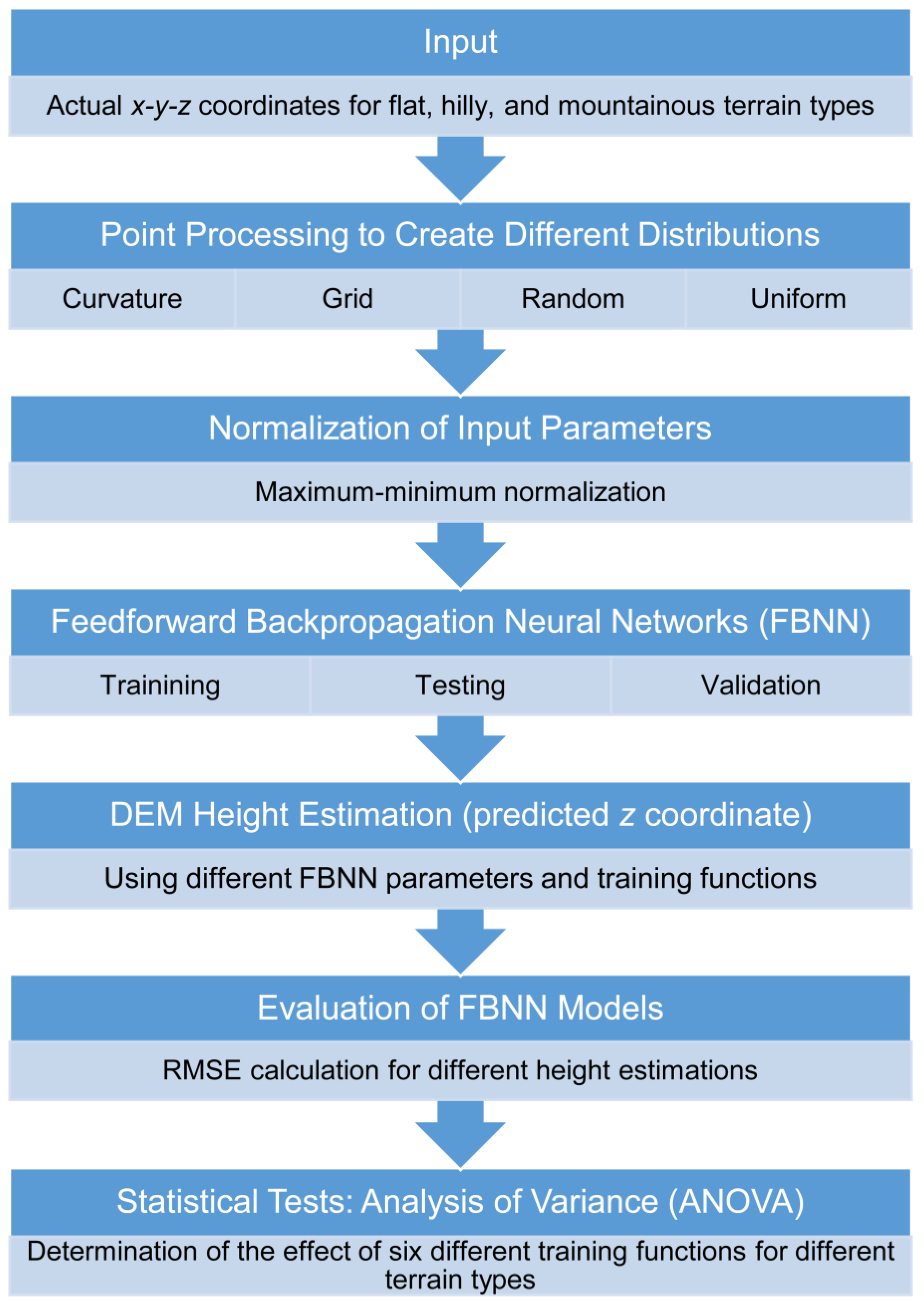
2. Materials and Methods
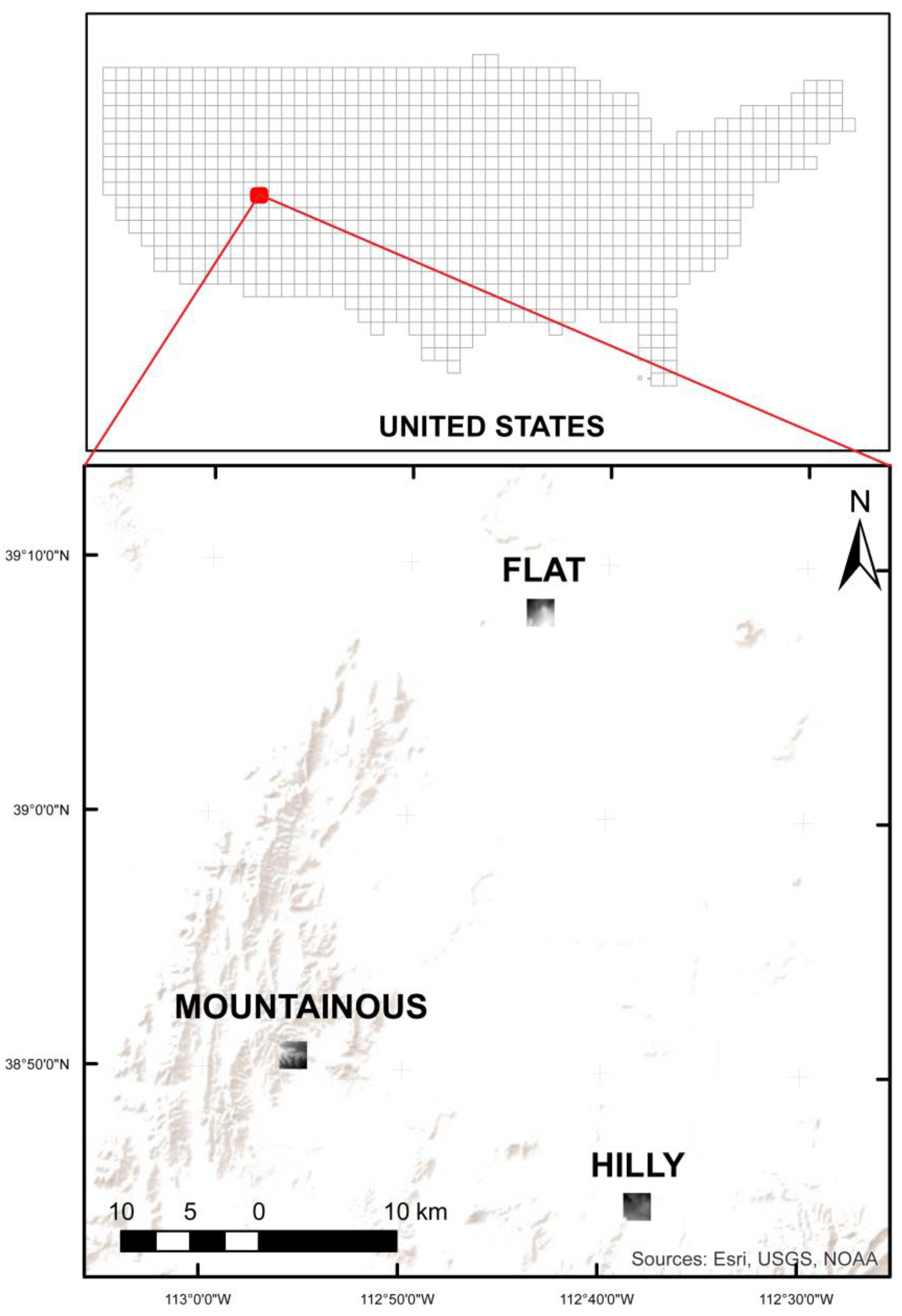
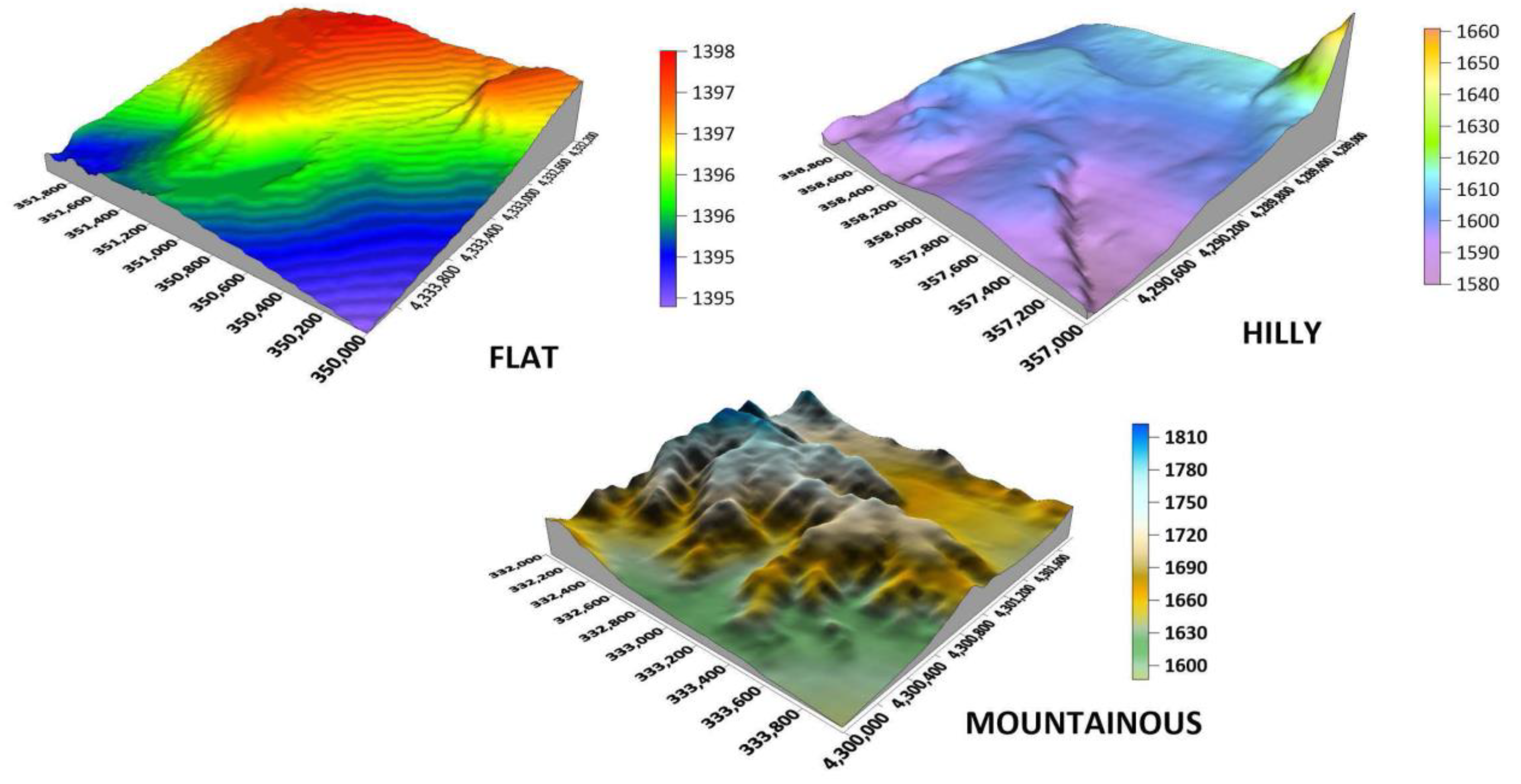
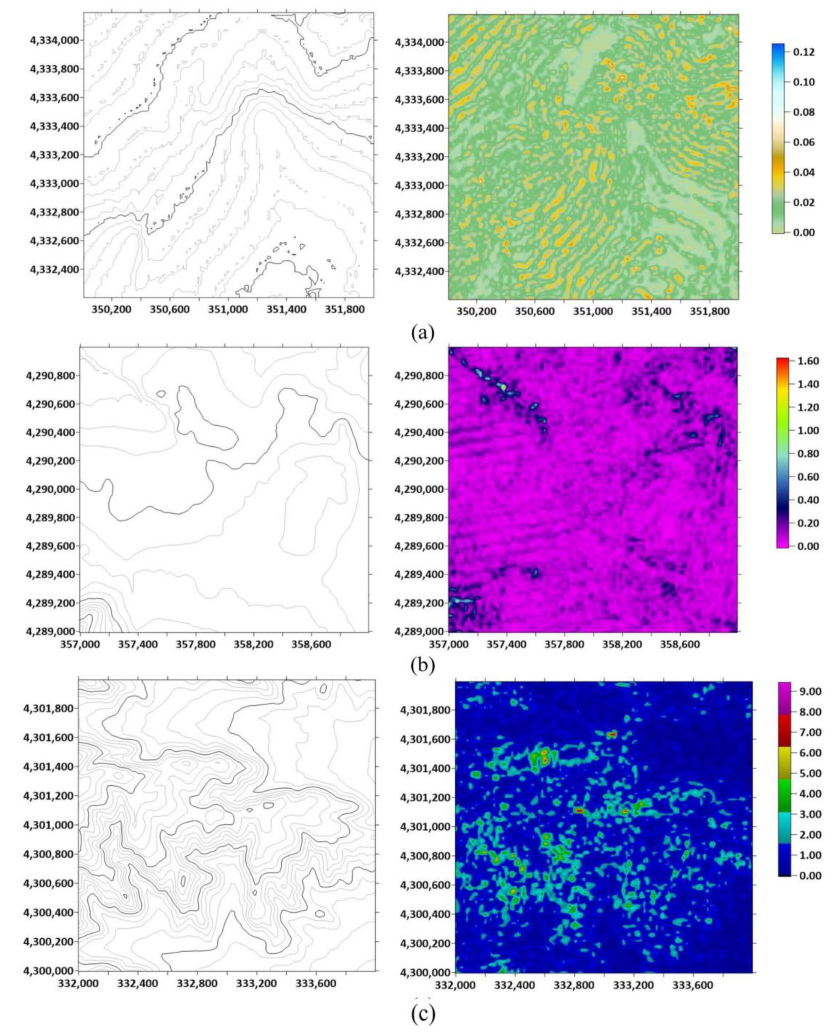
2.1. Experimental Data
2.2. Point Processing
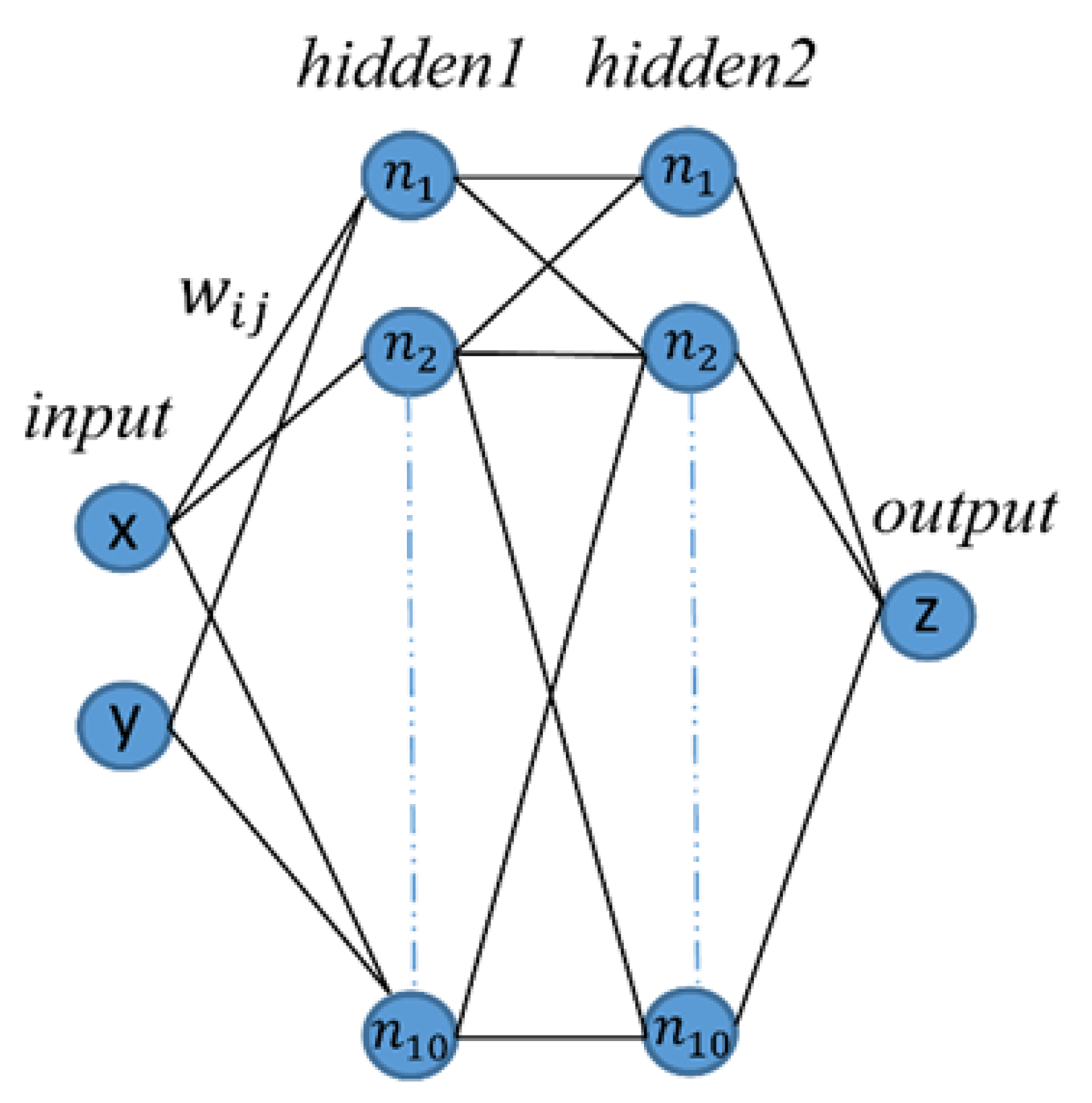
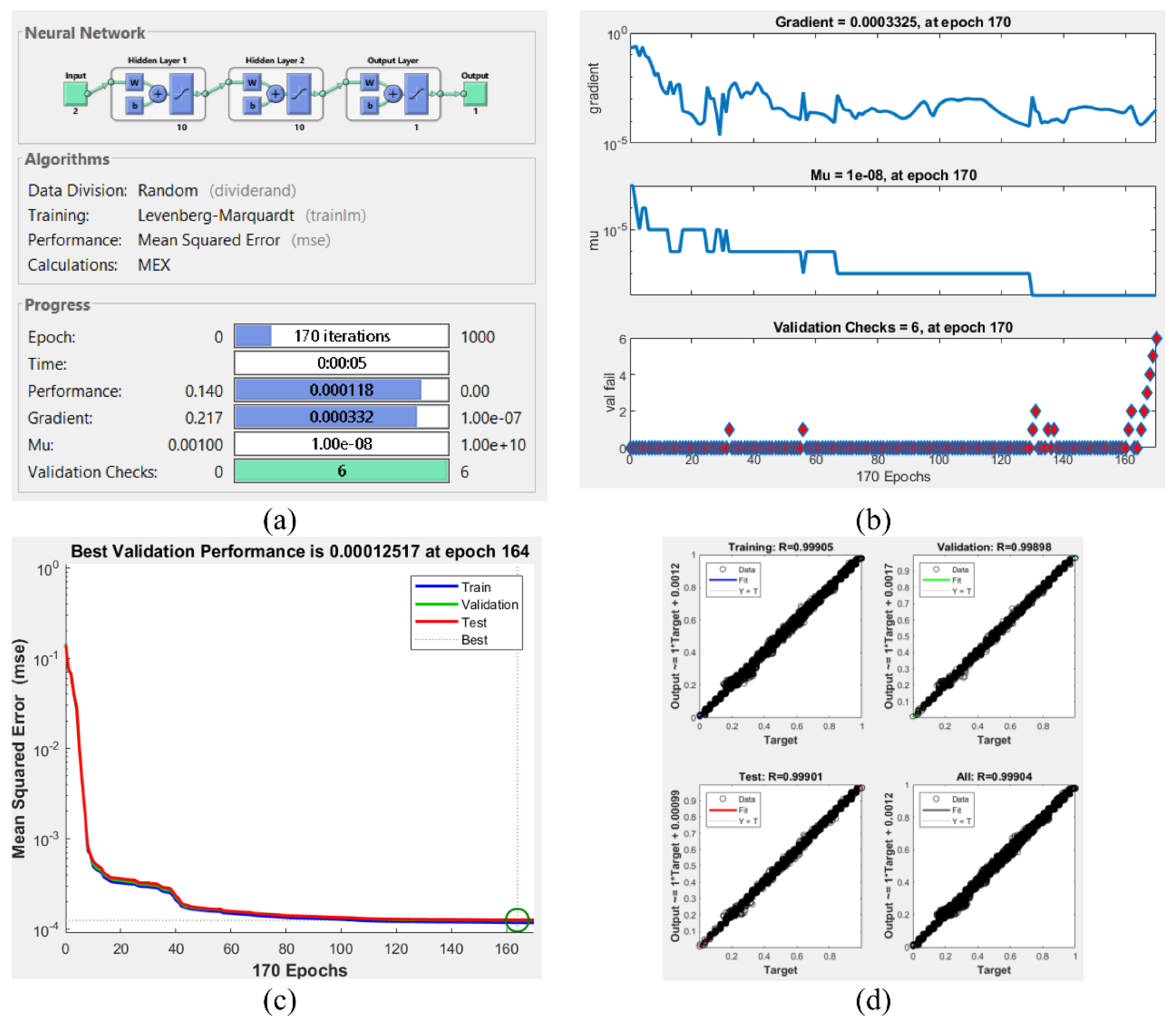
2.3. Feedforward Backpropagation Neural Networks
2.4. Statistical Tests: Analysis of Variance (ANOVA)
2.5. Software
3. Results and Discussion
4. Conclusions
Author Contributions
Funding
Data Availability Statement
Conflicts of Interest
References
- Chaplot, V.; Darboux, F.; Bourennane, H.; Leguédois, S.; Silvera, N.; Konngkeo, P. Accuracy of interpolation techniques for the derivation of digital elevation models in relation to landform types and data density. Geomorphology 2006, 77, 126–141. [Google Scholar] [CrossRef]
- Tu, J.; Yang, G.; Qui, P.; Ding, Z.; Mei, G. Comparative investigation of parallel spatial interpolation algorithms for building large-scale digital elevation models. PeerJ Comput. Sci. 2020, 6, e263. [Google Scholar] [CrossRef] [PubMed]
- Yan, L.; Tang, X.; Zhang, Y. High Accuracy Interpolation of DEM Using Generative Adversarial Network. Remote Sens. 2021, 13, 676. [Google Scholar] [CrossRef]
- Mitas, L.; Mitasova, H. Spatial interpolarion. In Geographical Information Systems: Principles, Techniques, Management and Applications, 2nd ed.; Longley, P.A., Goodchild, M.F., Maguire, D.J., Rhind, D.W., Eds.; John Wiley & Sons: Chichester, UK, 2005; pp. 481–492. [Google Scholar]
- Hu, P.; Liu, X.; Hu, H. Accuracy Assessment of Digital Elevation Models based on Approximation Theory. Photogramm. Eng. Remote Sens. 2009, 75, 49–56. [Google Scholar] [CrossRef]
- Guo, Q.; Li, W.; Yu, H.; Alvarez, O. Effects of topographic variability and Lidar sampling density on several DEM interpolation methods. Photogramm. Eng. Remote Sens. 2010, 76, 701–712. [Google Scholar] [CrossRef]
- Zhao, M. An indirect interpolation model and its application for digital elevation model generation. Earth Sci. Inform. 2020, 13, 1251–1264. [Google Scholar] [CrossRef]
- Alimissis, A.; Philippopoulos, K.; Tzanis, C.K.; Deligiorgi, D. Spatial estimation of urban air pollution with the use of artificial neural network models. Atmos. Environ. 2018, 191, 205–213. [Google Scholar] [CrossRef]
- Li, J.; Heap, A.D.; Potter, A.; Daniell, J.J. Application of machine learning methods to spatial interpolation of environmental variables. Environ. Model. Softw. 2011, 26, 1647–1659. [Google Scholar] [CrossRef]
- Appelhans, T.; Mwangomo, E.; Hardy, D.R.; Hemp, A.; Nauss, T. Evaluating machine learning approaches for the interpolation of monthly air temperature at Mt. Kilimanjaro, Tanzania. Spat. Stat. 2015, 14, 91–113. [Google Scholar] [CrossRef]
- Ruiz-Álvarez, M.; Alonso-Sarria, F.; Gomariz-Castillo, F. Interpolation of instantaneous air temperature using geographical and MODIS derived variables with machine learning techniques. ISPRS Int. J. Geo-Inf. 2019, 8, 382. [Google Scholar] [CrossRef]
- Leirvik, T.; Yuan, M. A machine learning technique for spatial Interpolation of solar radiation observations. Earth Sci. Space 2021, 8, e2020EA001527. [Google Scholar] [CrossRef]
- Gumus, K.; Sen, A. Comparison of spatial interpolation methods and multi-layer neural networks for different point distributions on a digital elevation model. Geod. Vestn. 2013, 57, 523–543. [Google Scholar] [CrossRef]
- Snell, S.E.; Gopal, S.; Kaufmann, R.K. Spatial Interpolation of Surface Air Temperatures Using Artificial Neural Networks: Evaluating Their Use for Downscaling GCMs. J. Cliımate 2000, 13, 886–895. [Google Scholar] [CrossRef]
- Charalambous, C. Conjugate gradient algorithm for efficient training of artificial neural networks. IEE Proc. G (Circuits Devices Syst.) 1992, 139, 301–310. [Google Scholar] [CrossRef]
- Moller, M.F. A scaled conjugate gradient algorithm for fast supervised learning. Neural Netw. 1993, 6, 525–533. [Google Scholar] [CrossRef]
- Bishop, C. Neural Networks for Pattern Recognition; Clarendon Press: Oxford, UK, 1995; pp. 116–148. [Google Scholar]
- Tavassoli, A.; Waghei, Y.; Nazemi, A. Comparison of Kriging and artificial neural network models for the prediction of spatial data. J. Stat. Comput. Simul. 2022, 92, 352–369. [Google Scholar] [CrossRef]
- Han, J.; Kamber, M.; Pei, J. Data Mining Concepts and Techniques; Elsevier: Waltham, MA, USA, 2012. [Google Scholar]
- Oztopal, A. Artificial neural network approach to spatial estimation of wind velocity data. Energy Convers. Manag. 2006, 47, 395–406. [Google Scholar] [CrossRef]
- Danesh, M.; Taghipour, F.; Emadi, S.M.; Sepanlou, M.G. The interpolation methods and neural network to estimate the spatial variability of soil organic matter affected by land use type. Geocarto Int. 2022, 37, 11306–11315. [Google Scholar] [CrossRef]
- Attoh-Okine, N.O. Analysis of learning rate and momentum term in backpropagation neural network algorithm trained to predict pavement performance. Adv. Eng. Softw. 1999, 30, 291–302. [Google Scholar] [CrossRef]
- Wong, K.; Dornberger, R.; Hanne, T. An analysis of weight initialization methods in connection with different activation functions for feedforward neural networks. Evol. Intell. 2022, 1–9. [Google Scholar] [CrossRef]
- Sharma, B.; Venugopalan, K. Comparison of neural network training functions for hematoma classification in brain CT images. IOSR J. Comput. Eng. 2014, 16, 31–35. [Google Scholar] [CrossRef]
- Kamble, L.; Pangavhane, D.; Singh, T. Neural network optimization by comparing the performances of the training functions -Prediction of heat transfer from horizontal tube immersed in gas–solid fluidized bed. Int. J. Heat Mass Transf. 2015, 83, 337–344. [Google Scholar] [CrossRef]
- Gesch, D. The National Elevation Dataset. Digital Elevation Model Technologies and Applications: The DEM Users Manual. In American Society for Photogrammetry and Remote Sensing; Maune, D., Ed.; Bethesda: Rockville, MD, USA, 2007; pp. 99–118. [Google Scholar]
- Strahler, A. Hypsometric (area-altitude) analysis of erosional topography. Bull. Geol. Soc. Am. 1952, 63, 1117–1142. [Google Scholar] [CrossRef]
- Melton, M. The geomorphic and palaeoclimatic significance of alluvial deposits in Southern Arizona. J. Geol. 1965, 73, 1–38. [Google Scholar] [CrossRef]
- Chorley, R. Spatial Analysis in Geomorphology; Routledge: London, UK, 1972. [Google Scholar]
- Sen, A.; Gumusay, M.U.; Kavas, A.; Bulucu, U. Programming an Artificial Neural Network Tool for Spatial Interpolation in GIS—A case study for indoor radio wave propagation of WLAN. Sensors 2008, 8, 5996–6014. [Google Scholar] [CrossRef] [PubMed]
- Hagan, M.; Menhaj, M. Training feed-forward networks with the Marquardt algorithm. IEEE Trans. Neural Netw. 1994, 5, 989–993. [Google Scholar] [CrossRef]
- Riedmiller, M.; Braun, H. A direct adaptive method for faster backpropagation learning: The RPROP algorithm. In Proceedings of the IEEE International Conference on Neural Networks, Orlando, FL, USA, 27–29 June 1994. [Google Scholar]
- Scales, L. Introduction to Non-Linear Optimization; Springer: New York, NY, USA, 1985. [Google Scholar]
- Hagan, M.; Demuth, H.; Beale, M. Neural Network Design; PWS Publishing: Boston, MA, USA, 1996. [Google Scholar]
- Beale, E. A derivation of conjugate gradients. In Numerical Methods for Nonlinear Optimization; Academic Press: London, UK, 1972; pp. 39–43. [Google Scholar]
- Tukey, J. Comparing individual means in the analysis of variance. Biometrics 1949, 5, 99–114. [Google Scholar] [CrossRef]
- Sparks, J. Expository notes on the problem of making multiple comparisons in a completely randomized design. J. Exp. Educ. 1963, 31, 343–349. [Google Scholar] [CrossRef]
- Zhang, Y.; Wenhao, Y. Comparison of DEM Super-Resolution Methods Based on Interpolation and Neural Networks. Sensors 2022, 22, 745. [Google Scholar] [CrossRef]
- Li, M.; Dai, W.; Song, S.; Wang, C.; Tao, Y. Construction of high-precision DEMs for urban plots. Ann. GIS 2023, 1–11. [Google Scholar] [CrossRef]
- Guth, P.L.; Van Niekerk, A.; Grohmann, C.H.; Muller, J.P.; Hawker, L.; Florinsky, I.V.; Gesch, D.; Reuter, H.I.; Herrera-Cruz, V.; Riazanoff, S.; et al. Digital Elevation Models: Terminology and Definitions. Remote Sens. 2021, 13, 3581. [Google Scholar] [CrossRef]


| Morphometric Parameters | Symbol | Description | Flat | Hilly | Mountain |
|---|---|---|---|---|---|
| Area | A | Measure in km2. | 4 km2 | 4 km2 | 4 km2 |
| The total length of 1 m interval contour lines | Measure in km. | 21.489 | 133.993 | 976.09 | |
| Relief [27] | R | The maximum and minimum height differences are given in meters. | 3.12 | 82.21 | 245.29 |
| Melton’s ruggedness number [28] | M | 0.0016 | 0.041 | 0.123 | |
| Slope [29] | S | , is the equidistance (1 m in this study) | 5.37 | 33.5 | 244.02 |
| Acronym | Algorithm | Description |
|---|---|---|
| lm | trainlm | Levenberg–Marquardt [31], |
| rp | trainrp | Resilient Backpropagation [32], |
| scg | trainscg | Scaled Conjugate Gradient [16], |
| cgf | traincgf | Fletcher-Powell Conjugate Gradient [33], |
| gd | traingd | Gradient Descent Backpropagation [34], |
| gdx | traingdx | Gradient descent with momentum and adaptive learning rule backpropagation [35]. |
| Parameters | Values |
|---|---|
| Number of layers | 2, 4, 6 |
| Number of hidden layer nodes | 10, 30, 80 |
| Transfer function | tanh |
| Epoch | 1000, 2000, 3000 |
| Performance function | RMSE |
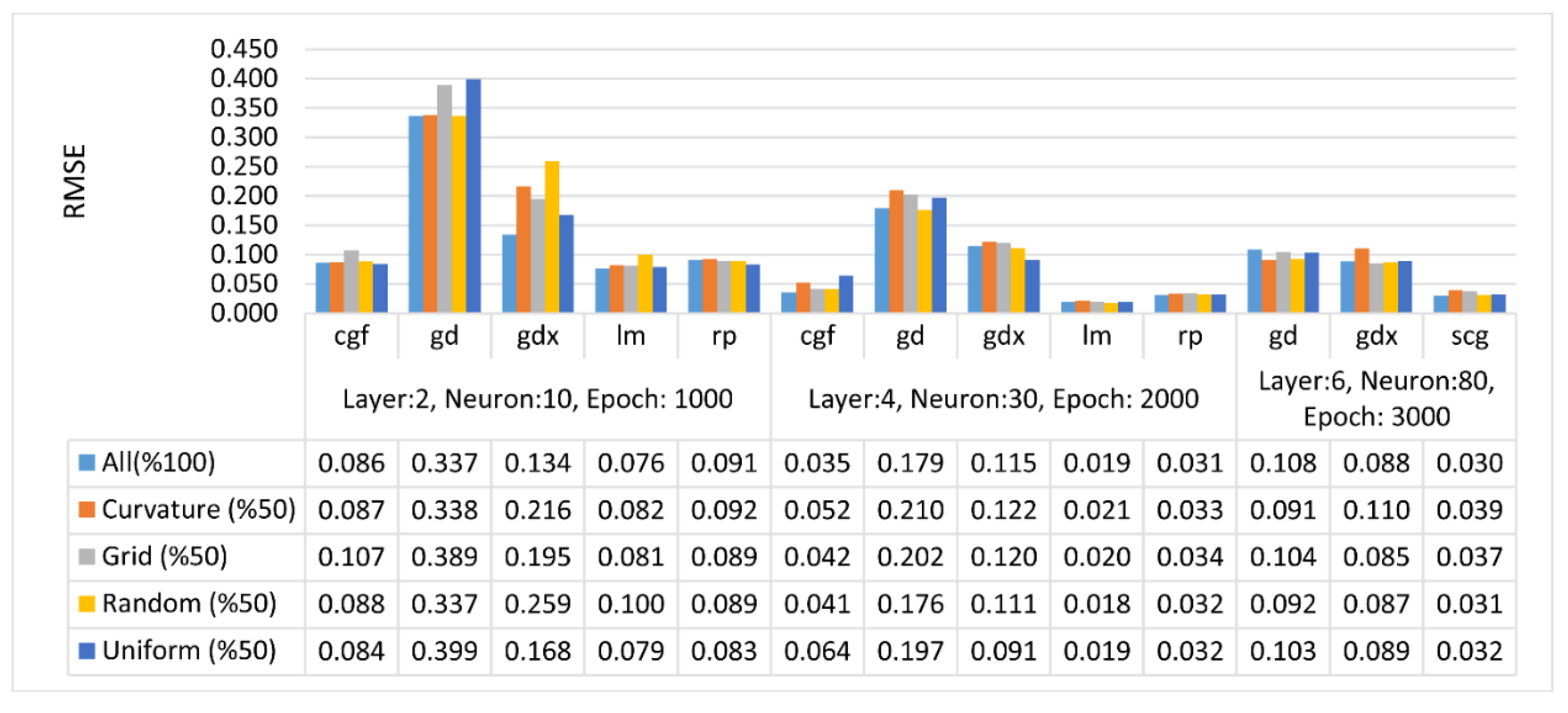
| Terrain | Distirbution | Layer:2, Neurons:10, Epoch: 1000 | Layer:4, Neurons:30, Epoch: 2000 | Layer:6, Neurons:80, Epoch: 3000 | ||||||||||
|---|---|---|---|---|---|---|---|---|---|---|---|---|---|---|
| Type | (%) | cgf | gd | gdx | lm | rp | cgf | gd | gdx | lm | rp | gd | gdx | scg |
| Flat | All | 518 | 1000 | 189 | 265 | 817 | 904 | 2000 | 150 | 536 | 1504 | 3000 | 132 | 672 |
| Curvature (50%) | 255 | 1000 | 182 | 199 | 936 | 439 | 2000 | 161 | 179 | 517 | 3000 | 116 | 209 | |
| Grid (50%) | 482 | 1000 | 184 | 209 | 643 | 437 | 2000 | 144 | 436 | 726 | 3000 | 142 | 203 | |
| Random (50%) | 388 | 1000 | 83 | 79 | 398 | 418 | 2000 | 160 | 705 | 734 | 3000 | 143 | 550 | |
| Uniform (50%) | 293 | 1000 | 178 | 241 | 667 | 340 | 2000 | 143 | 585 | 784 | 3000 | 132 | 550 | |
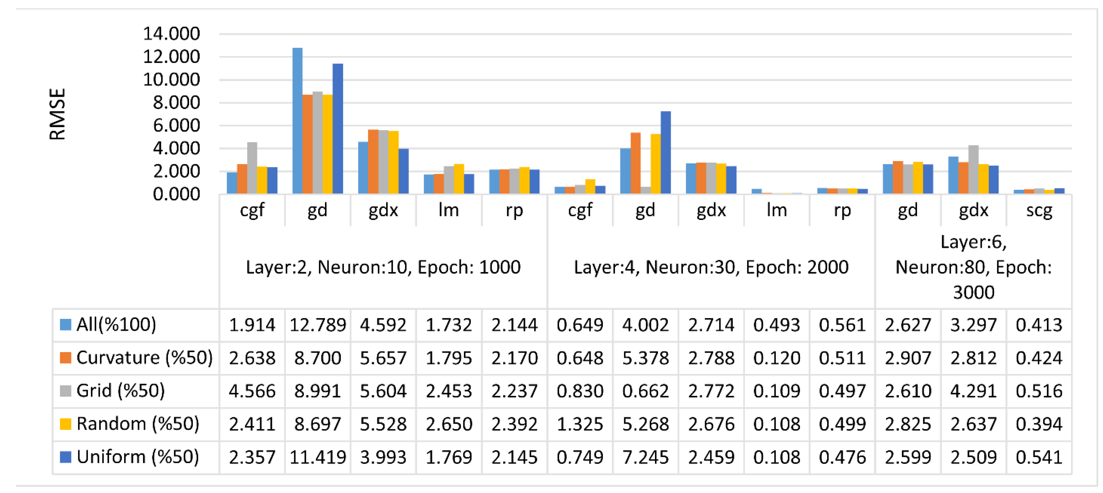
| Hilly | All | 678 | 1000 | 172 | 787 | 1000 | 774 | 2000 | 143 | 480 | 1000 | 3000 | 128 | 1074 |
| Curvature (50%) | 308 | 1000 | 63 | 989 | 532 | 62 | 2000 | 159 | 429 | 1243 | 3000 | 150 | 948 | |
| Grid (50%) | 141 | 1000 | 171 | 134 | 576 | 932 | 2000 | 161 | 663 | 2000 | 3000 | 22 | 522 | |
| Random (50%) | 277 | 1000 | 63 | 275 | 1000 | 252 | 2000 | 161 | 795 | 1833 | 3000 | 143 | 678 | |
| Uniform (50%) | 156 | 1000 | 172 | 376 | 688 | 482 | 2000 | 161 | 747 | 1493 | 3000 | 142 | 539 | |
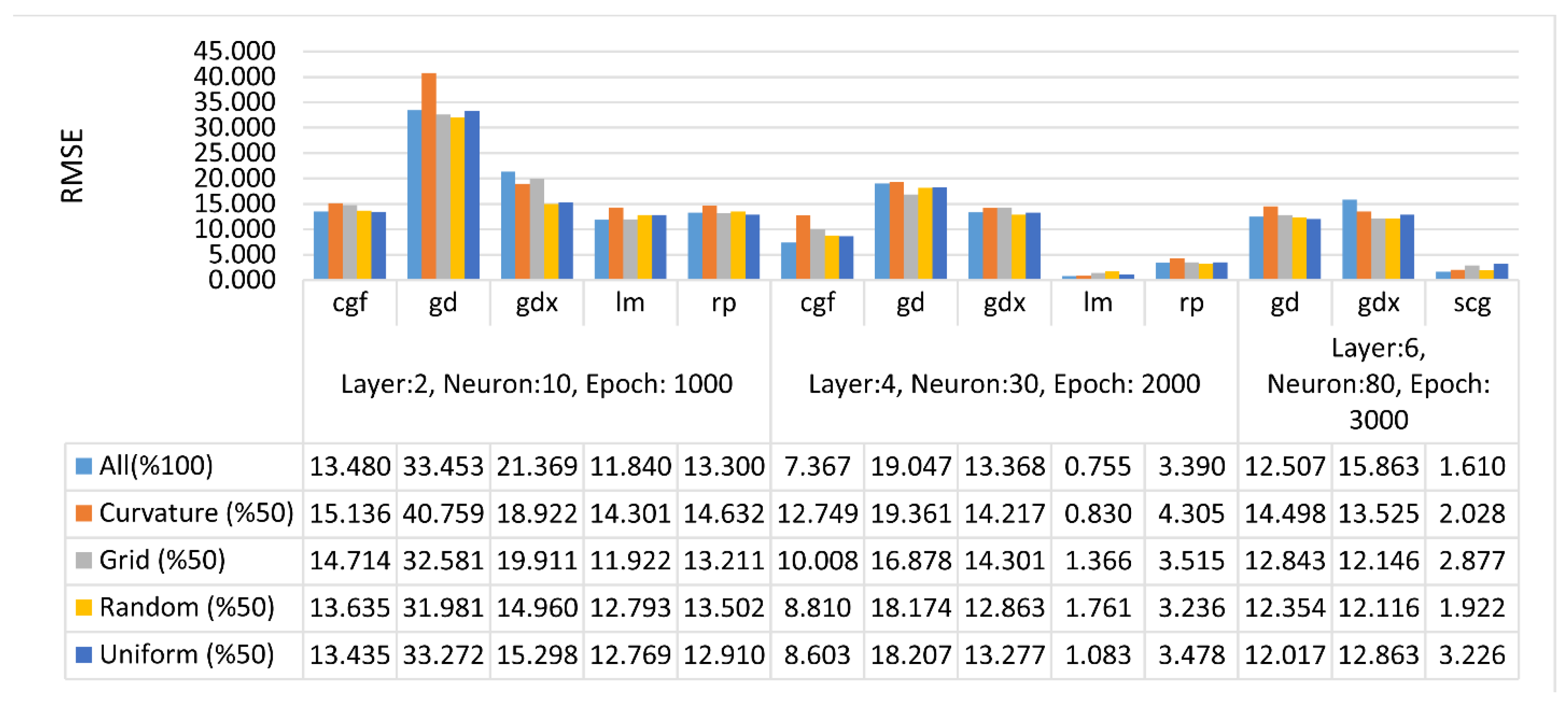
| Mountain | All | 279 | 1000 | 173 | 415 | 381 | 825 | 2000 | 152 | 1123 | 1681 | 3000 | 12 | 2755 |
| Curvature (50%) | 263 | 1000 | 163 | 48 | 233 | 278 | 2000 | 154 | 1043 | 2000 | 3000 | 132 | 2998 | |
| Grid (50%) | 337 | 1000 | 169 | 166 | 1000 | 453 | 2000 | 152 | 810 | 1763 | 3000 | 116 | 786 | |
| Random (50%) | 71 | 1000 | 168 | 281 | 220 | 320 | 2000 | 151 | 9 | 2000 | 3000 | 114 | 1800 | |
| Uniform (50%) | 232 | 1000 | 173 | 126 | 677 | 449 | 2000 | 2000 | 319 | 1738 | 3000 | 113 | 646 | |
| Terrain | Distirbution | Layer:2, Neurons:10, Epoch: 1000 | Layer:4, Neurons:30, Epoch: 2000 | Layer:6, Neurons:80, Epoch: 3000 | ||||||||||
|---|---|---|---|---|---|---|---|---|---|---|---|---|---|---|
| Type | (%) | cgf | gd | gdx | lm | rp | cgf | gd | gdx | lm | rp | gd | gdx | scg |
| Flat | All | 7 m 38 s | 6 m 6 s | 1 m 5 s | 2 m 58 s | 5 m 16 s | 26 m 19 s | 26 m 35 s | 1 m 56 s | 2 h 4 m 1 s | 30 m 56 s | 2 h 58 m 34 s | 8 m 38 s | 1 h 19 m 45 s |
| Curvature (50%) | 1 m 41 s | 2 m 56 s | 30 s | 1 m 14 s | 4 m 39 s | 5 m 44 s | 14 m 26 s | 51 s | 19 m 43 s | 6 m 21 s | 1 h 8 m 47 s | 4 m 42 s | 10 m 28 s | |
| Grid (50%) | 4 m 04 s | 3 m 33 s | 36 s | 51 s | 2 m 9 s | 6 m 27 s | 15 m 37 s | 1 m 5 s | 46 m 14 s | 5 m 22 s | 2 h 14 m 3 s | 3 m 29 s | 7 m 25 s | |
| Random (50%) | 3 m 39 s | 4 m 16 s | 21 s | 39 s | 2 m 25 s | 9 m 53 s | 23 m 42 s | 1 m 37 s | 2 h 36 m 27 s | 12 m 57 s | 1 h 10 m 18 s | 7 m 46 s | 30 m 0 s | |
| Uniform (50%) | 2 m 24 s | 3 m 26 s | 34 s | 1 m 22 s | 2 m 57 s | 6 m 50 s | 12 m 35 s | 58 s | 1 h 53 m 19 s | 8 m 21 s | 1 h 20 m 3 s | 4 m 26 s | 25 m 36 s | |
| Hilly | All | 12 m 41 s | 6 m 13 s | 1 m 30 s | 6 m 14 s | 6 m 16 s | 21 m 15 s | 41 m 29 s | 3 m 1 s | 51 m 55 s | 13 m 34 s | 2 h 29 m 3 s | 11 m 15 s | 2 h 7 m 12 s |
| Curvature (50%) | 3 m 14 s | 4 m 40 s | 17 s | 3 m 13 s | 1 m 42 s | 8 m 13 s | 21 m 1 s | 1 m 37 s | 40 m 55 s | 9 m 50 s | 1 h 30 m 6 s | 3 m 27 s | 43 m 56 s | |
| Grid (50%) | 2 m 7 s | 5 m 14 s | 59 s | 43 s | 1 m 54 s | 25 m 5 s | 15 m 12 s | 1 m 55 s | 2 h 21 m 51 s | 20 m 51 s | 1 h 45 m 2 s | 48 s | 27 m 26 s | |
| Random (50%) | 2 m 9 s | 3 m 16 s | 12 s | 1 m 1 s | 3 m 8 s | 3 m 47 s | 14 m 35 s | 1 m 7 s | 1 h 30 m 32 s | 12 m 01 s | 1 h 5 m 54 s | 3 m 4 s | 31 m 34 s | |
| Uniform (50%) | 1 m 55 s | 5 m 5 s | 51 s | 2 m 10 s | 3 m 12 s | 12 m 9 s | 24 m 39 s | 1 m 56 s | 2 h 31 m 43 s | 15 m 54 s | 1 h 31 m 45 s | 4 m 48 s | 28 m 15 s | |
| Mountain | All | 4 m 14 s | 12 m 33 s | 1 m 2 s | 2 m 49 s | 6 m 14 s | 24 m 25 s | 28 m 37 s | 4 m 16 s | 4 h 14 m 31 s | 25 m 44 s | 5 h 35 m 10 s | 39 s | 4 h 44 m 44 s |
| Curvature (50%) | 2 m 47 s | 4 m 25 s | 44 s | 11 s | 43 s | 3 m 37 s | 14 m 32 s | 1 m 34 s | 1 h 47 m 40 s | 36 m 5 s | 1 h 24 m 51 s | 2 m 59 s | 2 h 17 m 41 s | |
| Grid (50%) | 3 m 5 s | 3 m 15 s | 33 s | 2 m 4 s | 4 m 30 s | 7 m 51 s | 24 m 55 s | 1 m 4 s | 1 h 30 m 36 s | 22 m 32 s | 1 h 28 m 35 s | 3 m 15 s | 53 m 53 s | |
| Random (50%) | 40 s | 4 m 28 s | 41 s | 1 m 4 s | 41 s | 4 m 36 s | 14 m 55 s | 1 m 30 s | 1 m 19 s | 13 m 40 s | 1 h 43 m 24 s | 2 m 35 s | 1 h 31 m 13 s | |
| Uniform (50%) | 1 m 43 s | 3 m 8 s | 33 s | 30 s | 2 m 16 s | 7 m 17 s | 1 h 50 m 58 s | 25 m 48 s | 35 m 49 s | 12 m 38 s | 1 h 14 m 19 s | 2 m 47 s | 40 m 50 s | |
| Terrain | Distirbution | Layer:2, Neurons:10, Epoch: 1000 | Layer:4, Neurons:30, Epoch: 2000 | Layer:6, Neurons:80, Epoch: 3000 | ||||||||||
|---|---|---|---|---|---|---|---|---|---|---|---|---|---|---|
| Type | (%) | cgf | gd | gdx | lm | rp | cgf | gd | gdx | lm | rp | gd | gdx | scg |
| Flat | All | 0.0002 | 0.0295 | 0.0135 | 0.0000 | 0.0004 | 0.0006 | 0.0079 | 0.0256 | 0.0000 | 0.0000 | 0.0054 | 0.0358 | 0.0003 |
| Curvature (50%) | 0.0002 | 0.0296 | 0.0296 | 0.0000 | 0.0003 | 0.0021 | 0.0128 | 0.0163 | 0.0002 | 0.0001 | 0.0041 | 0.0265 | 0.0014 | |
| Grid (50%) | 0.0005 | 0.0501 | 0.0501 | 0.0001 | 0.0002 | 0.0009 | 0.0107 | 0.0250 | 0.0001 | 0.0001 | 0.0053 | 0.0246 | 0.0012 | |
| Random (50%) | 0.0004 | 0.0294 | 0.0294 | 0.0000 | 0.0004 | 0.0009 | 0.0100 | 0.0144 | 0.0003 | 0.0003 | 0.0041 | 0.0134 | 0.0003 | |
| Uniform (50%) | 0.0002 | 0.0351 | 0.0351 | 0.0000 | 0.0005 | 0.0049 | 0.0115 | 0.0182 | 0.0005 | 0.0005 | 0.0051 | 0.0249 | 0.0006 | |
| Hilly | All | 0.0003 | 0.0307 | 0.0122 | 0.0008 | 0.0002 | 0.0003 | 0.0093 | 0.0183 | 0.0001 | 0.0001 | 0.0048 | 0.0009 | 0.0004 |
| Curvature (50%) | 0.0008 | 0.0213 | 0.0633 | 0.0027 | 0.0002 | 0.0004 | 0.0119 | 0.0292 | 0.0000 | 0.0001 | 0.0053 | 0.0276 | 0.0012 | |
| Grid (50%) | 0.0052 | 0.0244 | 0.0230 | 0.0000 | 0.0002 | 0.0009 | 0.0004 | 0.0216 | 0.0001 | 0.0001 | 0.0048 | 0.2390 | 0.0007 | |
| Random (50%) | 0.0005 | 0.0214 | 0.0636 | 0.0001 | 0.0003 | 0.0018 | 0.0117 | 0.0200 | 0.0000 | 0.0001 | 0.0046 | 0.0340 | 0.0004 | |
| Uniform (50%) | 0.0015 | 0.0240 | 0.0080 | 0.0002 | 0.0002 | 0.0006 | 0.0022 | 0.0218 | 0.0000 | 0.0001 | 0.0048 | 0.0510 | 0.0004 | |
| Mountain | All | 0.0011 | 0.0214 | 0.0190 | 0.0005 | 0.0003 | 0.0080 | 0.0110 | 0.0243 | 0.0002 | 0.0001 | 0.0064 | 0.9680 | 0.0003 |
| Curvature (50%) | 0.0011 | 0.0326 | 0.0258 | 0.0001 | 0.0053 | 0.0195 | 0.0114 | 0.0314 | 0.0000 | 0.0002 | 0.0074 | 0.0659 | 0.0005 | |
| Grid (50%) | 0.0008 | 0.0341 | 0.0198 | 0.0001 | 0.0006 | 0.0101 | 0.0090 | 0.0343 | 0.0003 | 0.0001 | 0.0064 | 0.0949 | 0.0009 | |
| Random (50%) | 0.0008 | 0.0226 | 0.0203 | 0.0000 | 0.0007 | 0.0052 | 0.0117 | 0.0409 | 0.0072 | 0.0002 | 0.0059 | 0.0804 | 0.0009 | |
| Uniform (50%) | 0.0004 | 0.0391 | 0.0099 | 0.0000 | 0.0003 | 0.0033 | 0.0117 | 0.0197 | 0.0000 | 0.0002 | 0.0061 | 0.0742 | 0.0019 | |
| Terrain | Distirbution | Layer:2, Neurons:10, Epoch: 1000 | Layer:4, Neurons:30, Epoch: 2000 | Layer:6, Neurons:80, Epoch: 3000 | ||||||||||
|---|---|---|---|---|---|---|---|---|---|---|---|---|---|---|
| Type | (%) | cgf | gd | gdx | lm | rp | cgf | gd | gdx | lm | rp | gd | gdx | scg |
| Flat | All | 0.0008 | 0.0117 | 0.0019 | 0.0006 | 0.0009 | 0.0001 | 0.0033 | 0.0014 | 0.0000 | 0.0001 | 0.0012 | 0.0008 | 0.0001 |
| Curvature (50%) | 0.0008 | 0.0118 | 0.0048 | 0.0007 | 0.0009 | 0.0003 | 0.0046 | 0.0015 | 0.0000 | 0.0001 | 0.0009 | 0.0085 | 0.0002 | |
| Grid (50%) | 0.0012 | 0.0246 | 0.0039 | 0.0007 | 0.0008 | 0.0002 | 0.0042 | 0.0015 | 0.0000 | 0.0001 | 0.0011 | 0.0008 | 0.0001 | |
| Random (50%) | 0.0008 | 0.0117 | 0.0252 | 0.0010 | 0.0008 | 0.0002 | 0.0032 | 0.0013 | 0.0000 | 0.0001 | 0.0009 | 0.0008 | 0.0001 | |
| Uniform (50%) | 0.0007 | 0.0164 | 0.0029 | 0.0006 | 0.0007 | 0.0004 | 0.0040 | 0.0009 | 0.0000 | 0.0001 | 0.0011 | 0.0008 | 0.0001 | |
| Hilly | All | 0.0005 | 0.0242 | 0.0031 | 0.0004 | 0.0007 | 0.0001 | 0.0024 | 0.0011 | 0.0000 | 0.0000 | 0.0010 | 0.0393 | 0.0000 |
| Curvature (50%) | 0.0010 | 0.0112 | 0.0276 | 0.0005 | 0.0007 | 0.0001 | 0.0043 | 0.0012 | 0.0000 | 0.0000 | 0.0013 | 0.0012 | 0.0000 | |
| Grid (50%) | 0.0031 | 0.0121 | 0.0047 | 0.0009 | 0.0007 | 0.0001 | 0.0001 | 0.0012 | 0.0000 | 0.0000 | 0.0010 | 0.0594 | 0.0000 | |
| Random (50%) | 0.0009 | 0.0112 | 0.0271 | 0.0010 | 0.0008 | 0.0003 | 0.0041 | 0.0011 | 0.0000 | 0.0000 | 0.0012 | 0.0010 | 0.0000 | |
| Uniform (50%) | 0.0008 | 0.0193 | 0.0024 | 0.0005 | 0.0007 | 0.0001 | 0.0078 | 0.0009 | 0.0000 | 0.0000 | 0.0010 | 0.0009 | 0.0000 | |
| Mountain | All | 0.0030 | 0.0186 | 0.0076 | 0.0023 | 0.0029 | 0.0009 | 0.0060 | 0.0030 | 0.0000 | 0.0002 | 0.0026 | 0.0721 | 0.0000 |
| Curvature (50%) | 0.0038 | 0.0277 | 0.0060 | 0.0034 | 0.0036 | 0.0027 | 0.0063 | 0.0034 | 0.0000 | 0.0003 | 0.0035 | 0.0031 | 0.0001 | |
| Grid (50%) | 0.0036 | 0.0177 | 0.0066 | 0.0024 | 0.0029 | 0.0017 | 0.0048 | 0.0034 | 0.0000 | 0.0002 | 0.0028 | 0.0025 | 0.0001 | |
| Random (50%) | 0.0031 | 0.0170 | 0.0037 | 0.0027 | 0.0030 | 0.0013 | 0.0055 | 0.0028 | 0.0634 | 0.0002 | 0.0025 | 0.0024 | 0.0001 | |
| Uniform (50%) | 0.0030 | 0.0184 | 0.0039 | 0.0027 | 0.0028 | 0.0012 | 0.0055 | 0.0029 | 0.0000 | 0.0002 | 0.0024 | 0.0028 | 0.0002 | |
| Levene Statistic | df1 | df2 | Sig. | ||
|---|---|---|---|---|---|
| Training Functions | mountain | 15.108 | 5 | 59 | 0.000 |
| flat | 11.258 | 5 | 59 | 0.000 | |
| hilly | 13.249 | 5 | 59 | 0.000 | |
| Sum of Squares | df | Mean Square | F | Sig. | ||
|---|---|---|---|---|---|---|
| mountain | Between Groups | 2275.565 | 5 | 455.113 | 12.921 | 0.000 |
| Within Groups | 2078.207 | 59 | 35.224 | |||
| Total | 4353.772 | 64 | ||||
| flat | Between Groups | 0.286 | 5 | 0.057 | 13.894 | 0.000 |
| Within Groups | 0.243 | 59 | 0.004 | |||
| Total | 0.529 | 64 | ||||
| hilly | Between Groups | 229.796 | 5 | 45.959 | 11.282 | 0.000 |
| Within Groups | 240.348 | 59 | 4.074 | |||
| Total | 470.144 | 64 |
| (I) Functions | (J) Functions | Mean Difference (I–J) | Std. Error | Sig. | 95% Confidence Interval | |
|---|---|---|---|---|---|---|
| Lower Bound | Upper Bound | |||||
| traincgf | traingd | −10.069 | 2.656 | 0.021 | −19.071 | −1.067 |
| trainscg | 9.461 | 0.942 | 0.000 | 5.954 | 12.967 | |
| traingd | traincgf | 10.069 | 2.656 | 0.021 | 1.067 | 19.071 |
| trainlm | 13.920 | 3.143 | 0.003 | 3.658 | 24.182 | |
| trainrp | 13.314 | 3.005 | 0.003 | 3.474 | 23.155 | |
| trainscg | 19.530 | 2.521 | 0.000 | 10.710 | 28.349 | |
| traingdx | trainscg | 12.667 | 0.802 | 0.000 | 9.951 | 15.384 |
| trainlm | traingd | −13.920 | 3.143 | 0.003 | −24.182 | −3.658 |
| trainrp | traingd | −13.314 | 3.005 | 0.003 | −23.155 | −3.474 |
| trainscg | traincgf | −9.461 | 0.942 | 0.000 | −12.967 | −5.954 |
| traingd | −19.530 | 2.521 | 0.000 | −28.349 | −10.710 | |
| traingdx | −12.667 | 0.802 | 0.000 | −15.384 | −9.951 | |
| Trainings Functions | N | Mountain | Flat | Hilly | |||||||
|---|---|---|---|---|---|---|---|---|---|---|---|
| 1 | 2 | 3 | 1 | 2 | 3 | 1 | 2 | 3 | |||
| Tukey HSD a | trainscg | 5 | 2.333 | 0.034 | 0.457 | ||||||
| trainlm | 10 | 7.942 | 7.942 | 0.051 | 0.051 | 1.134 | 1.134 | ||||
| trainrp | 10 | 8.548 | 8.548 | 0.061 | 0.061 | 1.363 | 1.363 | ||||
| traincgf | 10 | 11.794 | 0.068 | 0.068 | 1.809 | 1.809 | |||||
| traingdx | 15 | 15.000 | 15.000 | 0.133 | 0.133 | 3.664 | 3.664 | ||||
| traingd | 15 | 21.862 | 0.218 | 5.781 | |||||||
| Sig. | 0.219 | 0.116 | 0.136 | 0.847 | 0.079 | 0.059 | 0.692 | 0.085 | 0.217 | ||
Disclaimer/Publisher’s Note: The statements, opinions and data contained in all publications are solely those of the individual author(s) and contributor(s) and not of MDPI and/or the editor(s). MDPI and/or the editor(s) disclaim responsibility for any injury to people or property resulting from any ideas, methods, instructions or products referred to in the content. |
© 2023 by the authors. Licensee MDPI, Basel, Switzerland. This article is an open access article distributed under the terms and conditions of the Creative Commons Attribution (CC BY) license (https://creativecommons.org/licenses/by/4.0/).
Share and Cite
Sen, A.; Gumus, K. Comparison of Different Parameters of Feedforward Backpropagation Neural Networks in DEM Height Estimation for Different Terrain Types and Point Distributions. Systems 2023, 11, 261. https://doi.org/10.3390/systems11050261
Sen A, Gumus K. Comparison of Different Parameters of Feedforward Backpropagation Neural Networks in DEM Height Estimation for Different Terrain Types and Point Distributions. Systems. 2023; 11(5):261. https://doi.org/10.3390/systems11050261
Chicago/Turabian StyleSen, Alper, and Kutalmis Gumus. 2023. "Comparison of Different Parameters of Feedforward Backpropagation Neural Networks in DEM Height Estimation for Different Terrain Types and Point Distributions" Systems 11, no. 5: 261. https://doi.org/10.3390/systems11050261