A New Decision Method of Flexible Job Shop Rescheduling Based on WOA-SVM

Abstract

Enterprise production is often interfered with by internal and external factors, resulting in the infeasible original production scheduling scheme. In terms of this issue, it is necessary to quickly decide the optimal production scheduling scheme after these disturbances so that the enterprise is produced efficiently. Therefore, this paper proposes a new rescheduling decision model based on the whale optimization algorithm and support vector machine (WOA-SVM). Firstly, the disturbance in the production process is simulated, and the dimensionality of the data from the simulation is reduced to train the machine learning model. Then, this trained model is combined with the rescheduling schedule to deal with the disturbance in the actual production. The experimental results show that the support vector machine (SVM) performs well in solving classification and decision problems. Moreover, the WOA-SVM can solve problems more quickly and accurately compared to the traditional SVM. The WOA-SVM can predict the flexible job shop rescheduling mode with an accuracy of 89.79%. It has higher stability compared to other machine learning methods. This method can respond to the disturbance in production in time and satisfy the needs of modern enterprises for intelligent production.

1. Introduction

In a flexible job shop, a variety of sudden disturbances often occur, such as machine failure, urgent order insertion, part arrival time deviation, processing time delay, etc. These disturbances are characterized by random and discrete distributions [1], and these disturbances cannot be predicted in advance. Therefore, the rescheduling procedure after the disturbance must be timely and accurate, so as not to delay the delivery term and bring losses to the enterprise.

Numerous academics have undertaken studies from the perspectives of optimization algorithms and intelligent scheduling in order to meet the needs of automation and intelligent production of modern enterprise shop scheduling. As an earlier intelligent optimization algorithm, the Genetic algorithm (GA) has been improved by many scholars, and has been proven to be quite effective at solving the shop scheduling problem. For example, Dai et al. [2] established a multi-objective optimization model to minimize energy consumption and completion time for flexible job-shop scheduling problems with transportation constraints. Zhang et al. [3] ameliorated the genetic programming super-heuristic algorithm for dynamic flexible job shop scheduling and proposed an individual adaptation strategy. Liu et al. [4] proposed a genetic algorithm based on the multi-objective and multi-population framework for the multi-objective job-shop scheduling problem. Yan et al. [5] discussed the influence of finite transportation conditions on flexible job-shop scheduling problems and improved the genetic algorithm. Kacem et al. [6,7] used the local heuristic method for initialization, and then used the genetic algorithm for multi-objective optimization of the initial solution. For solving multi-objective problems, Wu et al. [8] and Yu et al. [9] combined genetic algorithms with local search algorithms, such as the immune algorithm, to amplify the ability of local search in the algorithm. On the basis of certain research studies on shop scheduling and algorithms, many scholars seek more suitable algorithms. Afsar et al. [10] proposed a multi-objective optimization model and a new enhanced mode gene algorithm for the green-scheduling problem of the job shop. Alkhateeb et al. [11] integrated the optimization operator of the simulated annealing algorithm into the Cuckoo search algorithm and proposed a discrete simulated annealing algorithm to solve the job-shop problem. Caldeira et al. [12] proposed a multi-objective discrete Jaya algorithm for solving scheduling problems based on the Pareto multi-objective algorithm. Ibrahim et al. [13] proposed an efficient solution strategy with better performance for job-shop scheduling problems by combining the artificial algae algorithm with the differential evolution algorithm. Brandimarte et al. [14], aiming to solve the multi-objective Flexible Job Shop Problem (FJSP), used the assignment rule to solve the machine selection problem, and then adopted tabu search to solve the shop scheduling problem. Baykasoglu et al. [15] studied the dynamic flexible job-shop scheduling problem under new order arrival, delivery date change, machine failure, order cancellation, and urgent order arrival. Mohan et al. [16] summarized the development of a dynamic job-shop scheduling problem, and pointed out that future research should be in-depth in the direction of integration, practicability, multi-targeting, and networking. Although the algorithm in the job-shop scheduling problem has been the subject of extensive research, it is rarely applied to actual or intelligent production in enterprises. As a result, the research focus of job-shop scheduling has changed to successful algorithm implementation, intelligent scheduling implementation in production, and intelligent scheduling achievement.

In order to keep high decision accuracy, make shop scheduling intelligent, and reduce the artificial experience judgment operation, research should be conducted from the viewpoints of machine learning and deep learning. Priore et al. [17] summarized scheduling methods of machine learning to select the most appropriate scheduling rules for a flexible manufacturing system at any given time. Wang et al. [18] proposed a dynamic scheduling method based on deep reinforcement learning and adopted Proximal Policy Optimization (PPO) to find the optimal scheduling strategy. Zhang et al. [19] suggested a graph neural network-based approach to integrate the states encountered in the solving process through end-to-end deep reinforcement learning. Chen et al. [20] proposed a self-learning genetic algorithm (SLGA) and made an intelligent adjustment of its key parameters using reinforcement learning. Cao et al. [21] aimed at the problem of wireless network resource allocation, and proposed a machine learning method based on support vector machines and deep belief networks to directly calculate approximate solutions. Weckman et al. [22] used the genetic algorithm to investigate a neural network scheduler for job shop scheduling. Based on a graph neural network, Hameed [23] proposed a new method to solve job-shop scheduling problems by using deep reinforcement learning. Inspired by the idea of machine learning to job-shop scheduling, many scholars have further studied digital twinning and cloud computing. Fang et al. [24] developed a new shop scheduling method based on digital twin (DT) to reduce scheduling deviation. Zhang et al. [25] introduced digital twin technology to further integrate the physical space and virtual space of the workshop for realizing dynamic scheduling. From the standpoint of cloud computing, Tong et al. [26] proposed a task scheduling algorithm combining Q learning and heterogeneous earliest completion time method. Morariu et al. [27] proposed a machine learning method for reality perception and optimization in the cloud environment to reduce the cost of cloud computing implementation and deployment for manufacturing enterprises. Liu et al. [28] suggested a user scheduling algorithm for data acquisition in edge learning, taking into account communication reliability and information volume of data samples. Ghasemi et al. [29] introduced evolutionary learning to the simulation method of stochastic optimization. In addition to the above research, many scholars also study shop scheduling from other perspectives and technical means. Amiri et al. [30] presented an algorithm iteration that can simulate stochastic gradient descent to significantly reduce the average completion time, aiming at the computational task scheduling problem of multiple workers in large-scale distributed learning problems. Faraji et al. [31] proposed a new power management system based on weather and load forecasting for optimal day-ahead automatic scheduling and operation of the microgrid. Müller et al. [32] studied five constraint programming solvers and developed a prediction method of the best solver according to the instance features or parameters for a given problem. Jun et al. [33] suggested a method, which could be called Random Forest for Obtaining Rules for Scheduling (RANFORS), to extract scheduling rules from optimal scheduling. Li et al. [34] proposed an elite non-dominated sorting hybrid algorithm to solve multi-objective flexible job shop scheduling problems with sequence-dependent setup time and cost.

Obviously, machine learning, which is an important means to realize precision and intelligence in modern intelligent manufacturing enterprises, can be applied to find rules and predict development from previous production experience and data.

Therefore, this paper develops a prediction method based on an improved whale optimization algorithm and support vector machine (WOA-SVM) for rescheduling mode decisions in a flexible job shop. A big sample of data is produced when there is a random disturbance. A variety of machine learning methods are used to train and predict the data, and are compared with the method proposed in this paper. It is proved that the proposed method can respond to rescheduling decisions quickly.

2. Problem Description

Compared with the traditional Job-shop Scheduling Problem (JSP), there are operations of assigning processes to machines in FJSP [35]. FJSP means the $n$ workpieces to be processed on $m$ machines, and each process can be carried out on one or more machines. The problem constraints are as follows:

• The processing sequence of the same workpiece is fixed;
• There is no sequential connection between any process of different workpieces;
• Each process can only be processed on one machine at the same time;
• Each machine can only process one process at the same time;
• The processing priority of different workpieces is the same;
• The processing time of the same process in different machines can be different;
• The processing cannot be interrupted.

Optional machine examples of the process can be seen in

Table 1. Optional machine examples of the process.

	Process 1	Process 2	Process 3
Workpiece 1	$M_1$, $M_4$	$M_4$	$M_2$, $M_3$
Workpiece 2	$M_2$	$M_1$, $M_3$	$M_4$
Workpiece 3	$M_4$	$M_2$, $M_3$	$M_1$, $M_3$
Workpiece 4	$M_1$, $M_4$	$M_3$	-

.

Table 2. Example of processing time.

	Process 1	Process 2	Process 3
Workpiece 1	[3, 4]	9	[9, 10]
Workpiece 2	6	[8, 8]	4
Workpiece 3	5	[7, 8]	[7, 6]
Workpiece 4	[7, 7]	3	-

shows examples of processing time. $O_{ij}$ represents the $j$ process of the $i$ workpiece. Taking process $O_{101}$ as an example, it can be carried out on machine 1 or machine 4, and its processing time on the two machines is 3 min and 4 min, respectively. According to Table 1 and Table 2, the double-layer coding genetic algorithm [35,36] is used to generate the original scheduling scheme, as shown in Figure 1.

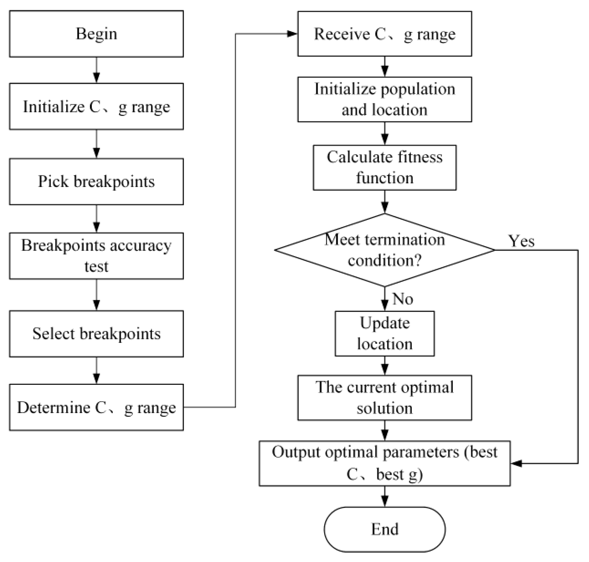
3. Rescheduling Mode Selection Model Based on Machine Learning

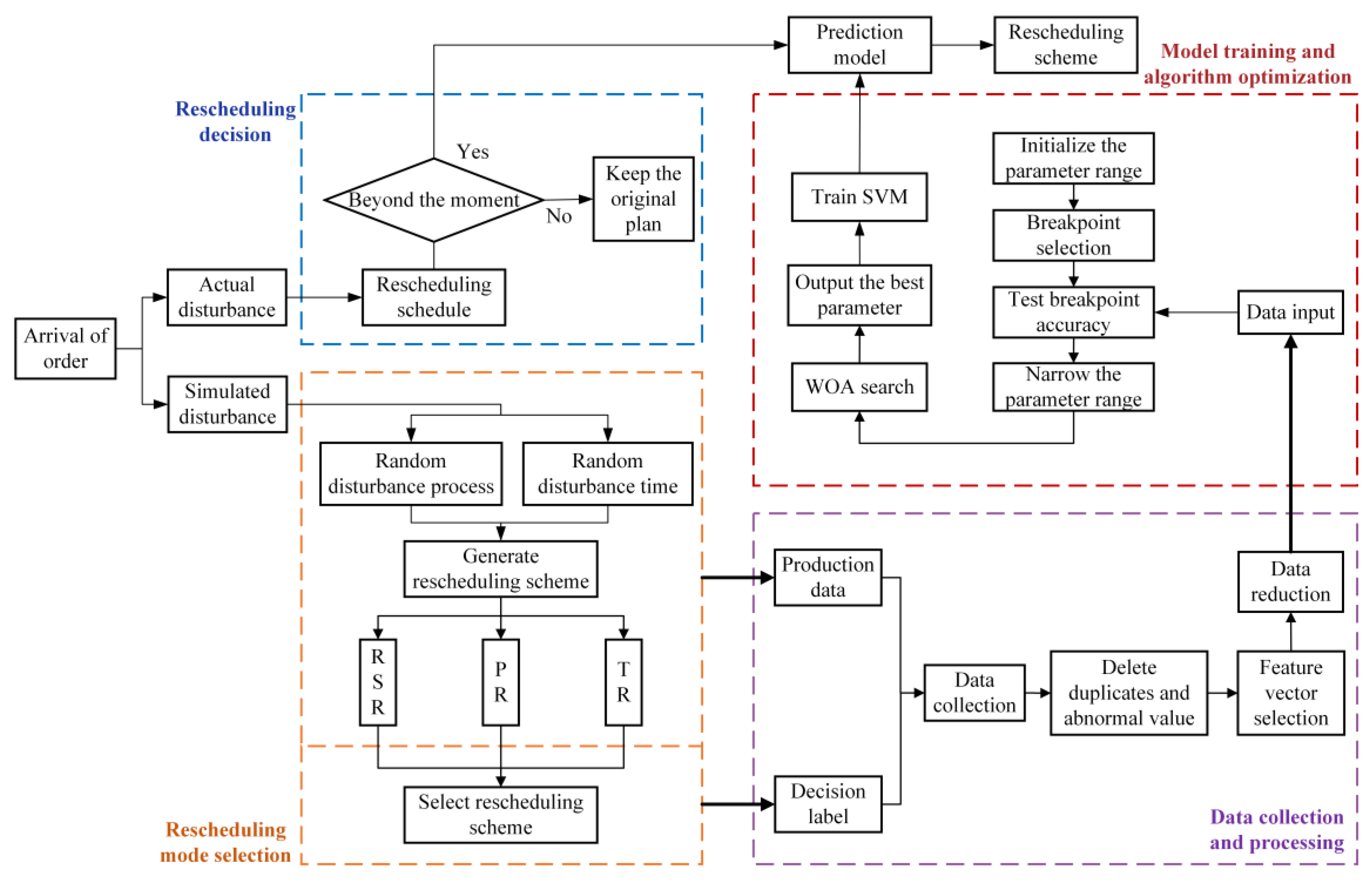
For realizing fast and accurate rescheduling mode decisions, the rescheduling mode selection model based on machine learning is adopted. Its framework is displayed in Figure 2. Firstly, it is assumed that a disturbance occurs during processing. Rescheduling mode selection is carried out, and then the data collection and processing start. These steps are repeated several times. Next, model training and algorithm optimization are performed and output the prediction model. Lastly, the actual disturbance can be disposed of in the rescheduling decision module when it happens in the actual production process.

3.1. Rescheduling Decision

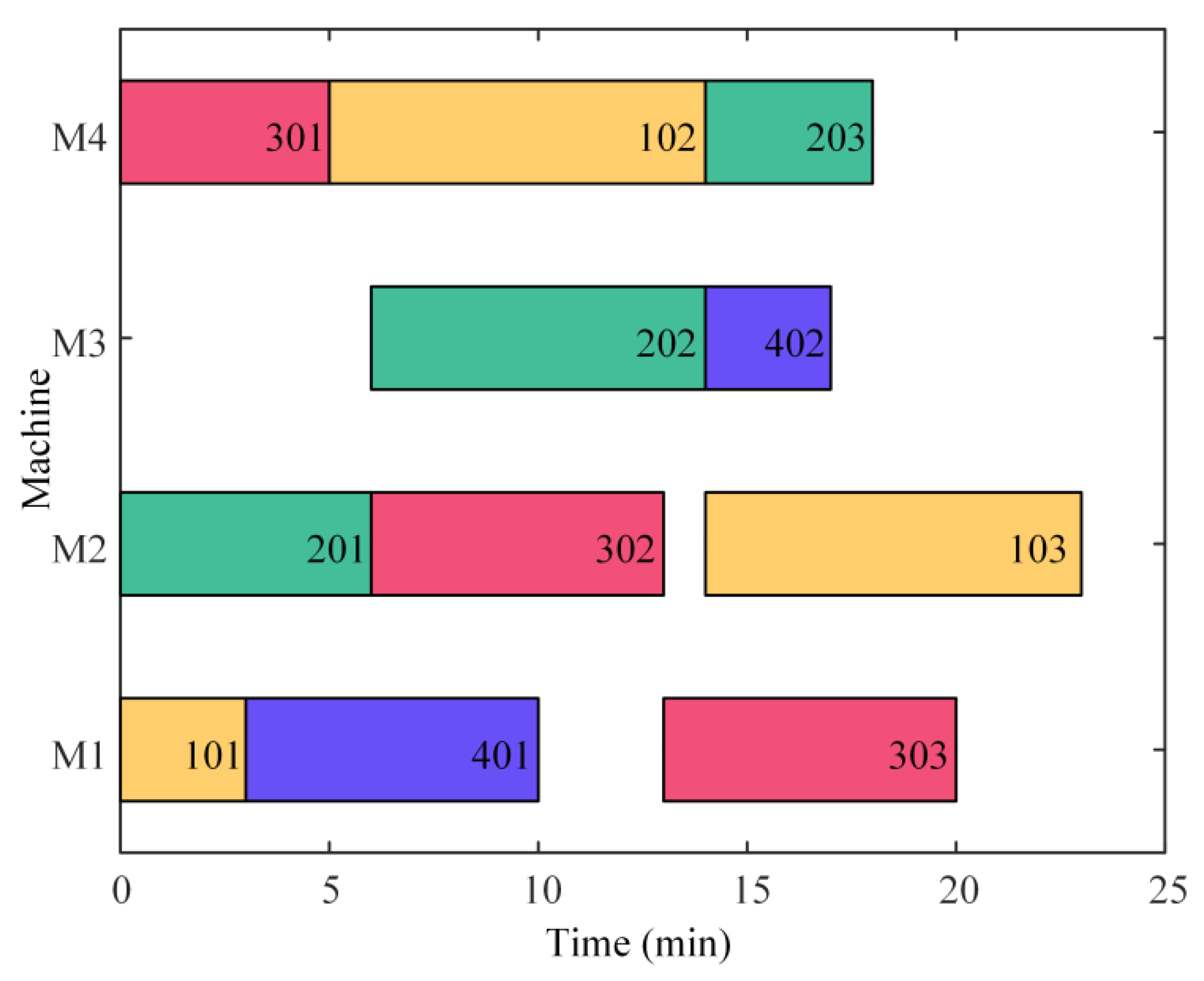
When a disturbance occurs in actual production, we need to estimate the effect of the disturbance and the necessity of rescheduling, first. Therefore, a rescheduling schedule is constructed to define the time limit for each process in which rescheduling is triggered.

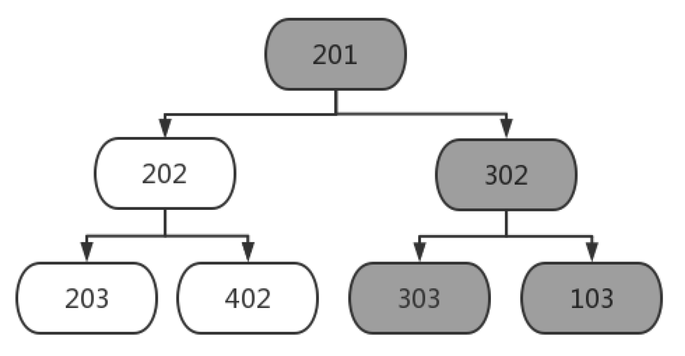
The dynamic correlation among processes in the scheduling scheme [37] is constructed, and the linkage influence brought by the disturbance of a certain process has been described in Figure 1. Figure 3 displays the correlation among processes. When $O_{201}$ is disturbed, the processes $O_{202}$ and $O_{302}$ will be influenced directly, and the processes $O_{203}$, $O_{402}$, $O_{303}$ and $O_{103}$ will be influenced indirectly. It is obvious that each process directly affects at most two processes, including the next adjacent process on the machine and the next adjacent process on the workpiece. Therefore, two dimensions are used to summarize the two different types of impacts (machine dimension and workpiece dimension).

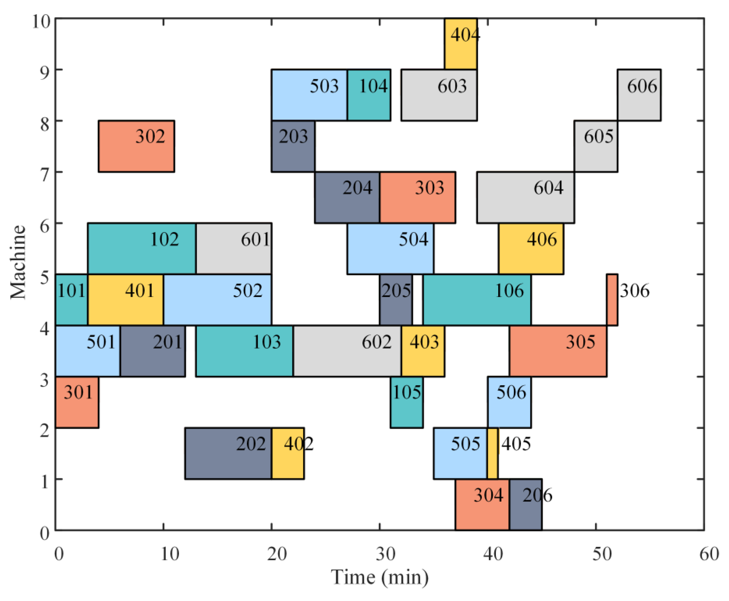
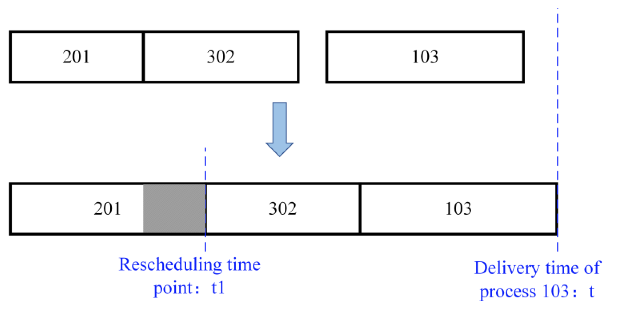
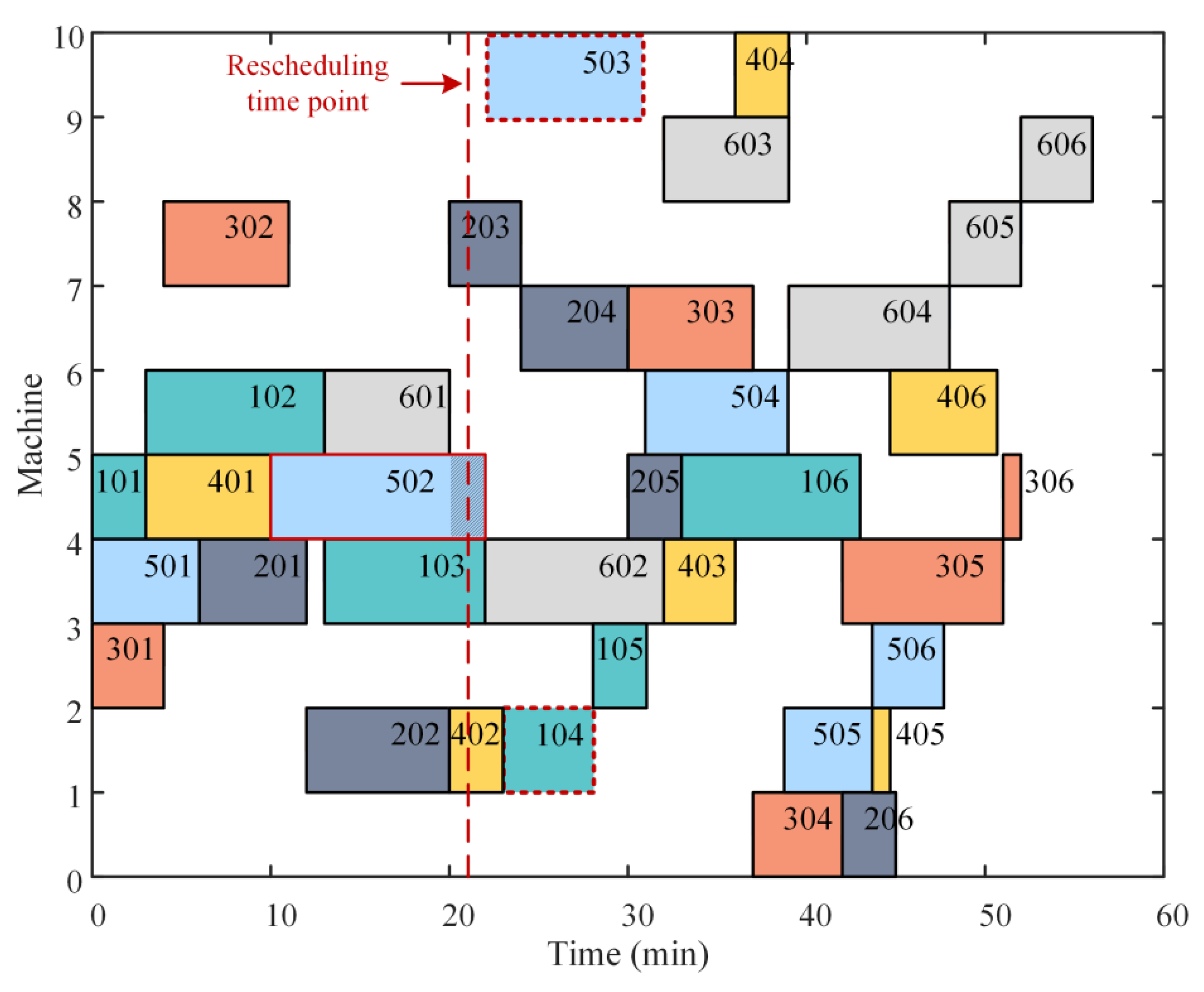
The latest tolerated completion time of each working procedure can be derived backwards from the connection between the two dimensions of the machine and the workpiece, if each workpiece’s delivery date or the latest acceptable completion time can be determined. Figure 4 demonstrates the determination of the rescheduling time point. If the delivery time of process 103 is $t$, it can still be completed, although process 201 is delayed to time point $t1$. Therefore, $t1$ can be defined as the rescheduling time point of process 201.

The above example simply illustrates that the calculation of the rescheduling time point of a certain process needs to take into account the delivery time of all the workpieces and the linkage effect of the two dimensions. Then, the rescheduling time points of all processes are calculated, and the rescheduling schedule is constructed. The initial scheduling scheme is maintained if the disruption in actual production does not last longer than the associated rescheduling time. If not, the production plan needs to be rescheduled.

3.2. Rescheduling Mode Selection

When the production order arrives, the rescheduling mode selection consists of the following steps. Firstly, the original scheduling scheme and rescheduling schedule are generated. Secondly, the disturbance process and the disturbance duration, which can trigger rescheduling, are randomly generated. Finally, based on the three scheduling modalities, the three rescheduling strategies are constructed.

There are three rescheduling modes: right shift rescheduling (RSR), partial rescheduling (PR), and total rescheduling (TR) [1,2]. RSR means that the sequence and machine among working procedures will not be changed, but the processing start time will be adjusted. PR can be used to rearrange the affected processes that have not started at the rescheduling time point, and maintain the original scheme for other unaffected processes. TR is a complete rescheduling of all processes that have not started at a rescheduling point in time. RSR has the least impact on the original scheduling scheme among the three rescheduling techniques, followed by PR, while TR has the greatest impact.

After the disturbance occurs, three rescheduling schemes are generated, and their corresponding maximum completion times $T_{max1}$, $T_{max2}$, and $T_{max3}$ are obtained to make rescheduling decisions:

$$f=min\left(T_{max1}+l,T_{max2}+2l,T_{max3}+3l\right)$$

(1)

$$type=\{\begin{array}{c}a, f=T_{max1}+l \\ b, f=T_{max2}+2l\\ c, f=T_{max3}+3l\end{array}$$

(2)

In Formula (1), $l$ represents a minimal positive number. It can be used to choose an optimal rescheduling scheme when the $T_{max}$ of different rescheduling modes is equal. $f$ represents the minimum completion time of the three rescheduling schemes. The corresponding schemes are selected through the $type$ function defined in Formula (2). $a$, $b$, and $c$, respectively, represent the three rescheduling schemes. They are decision labels in the data collection and processing module.

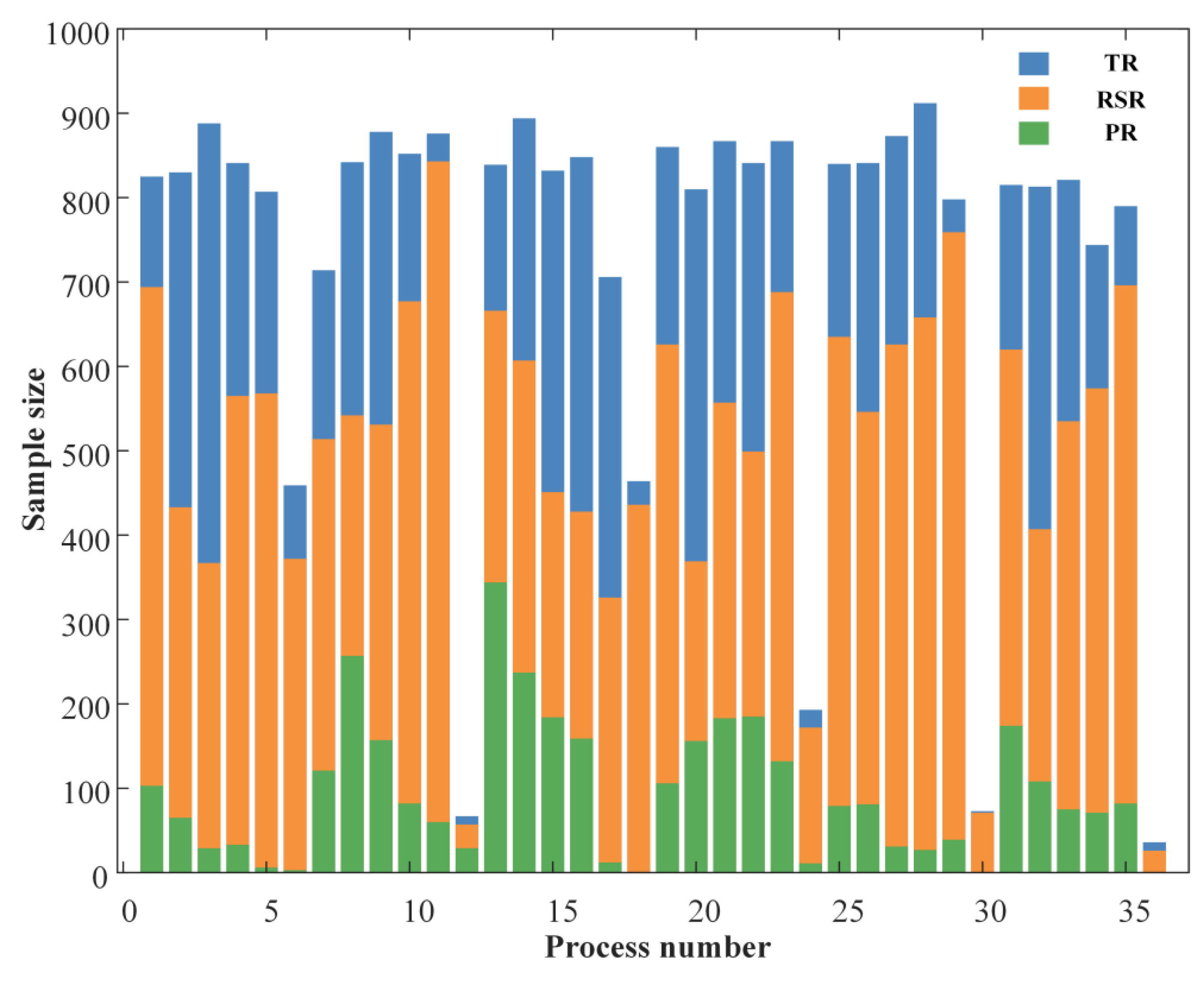
3.3. Data Collection and Processing

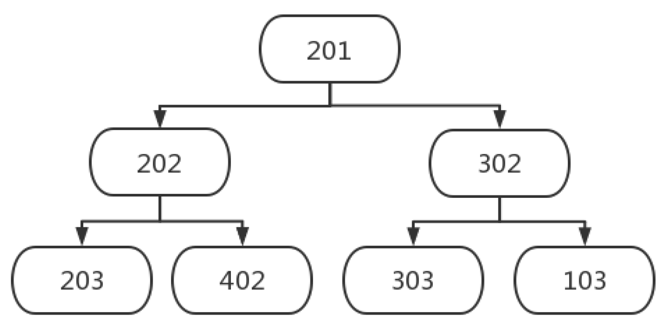
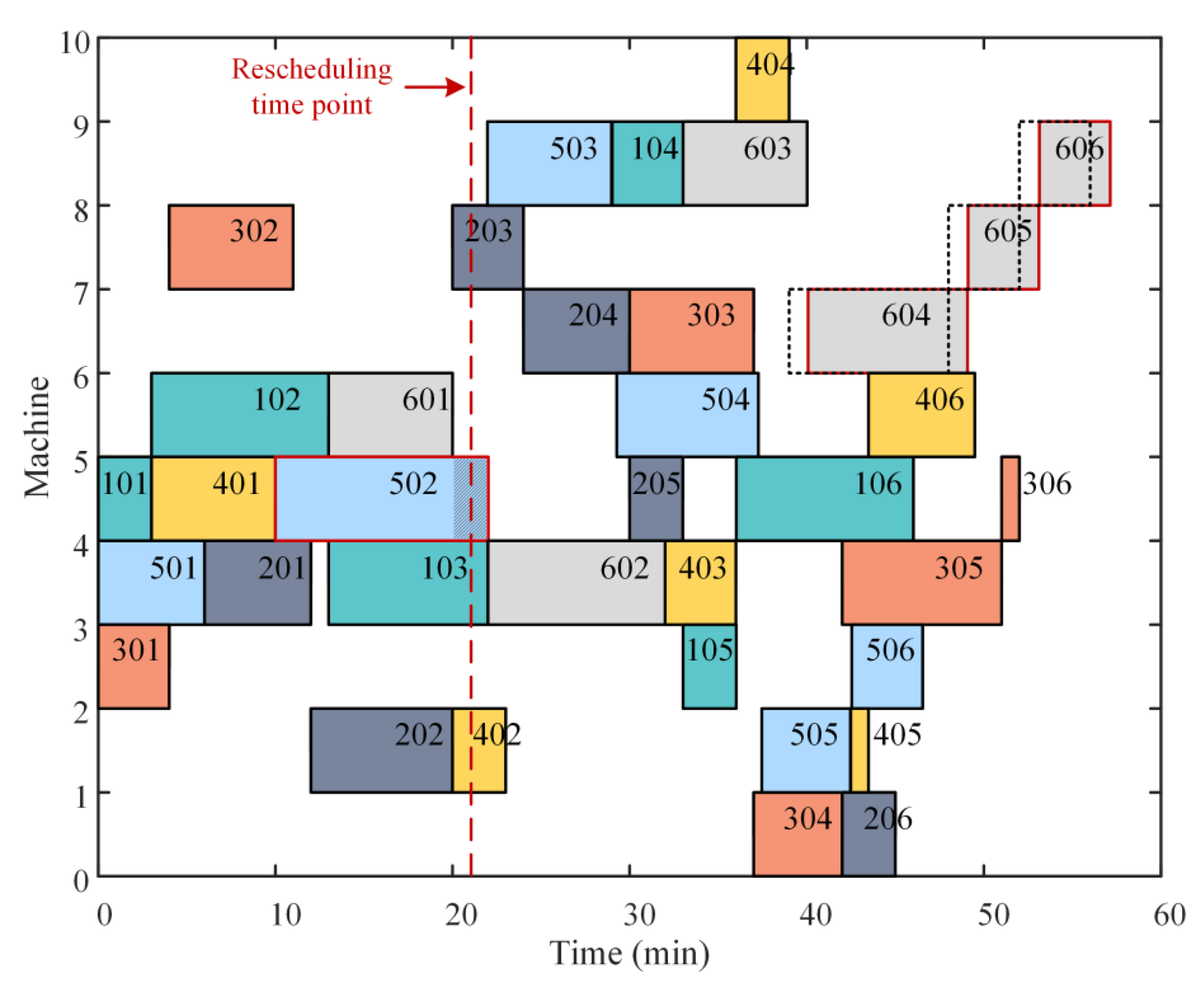
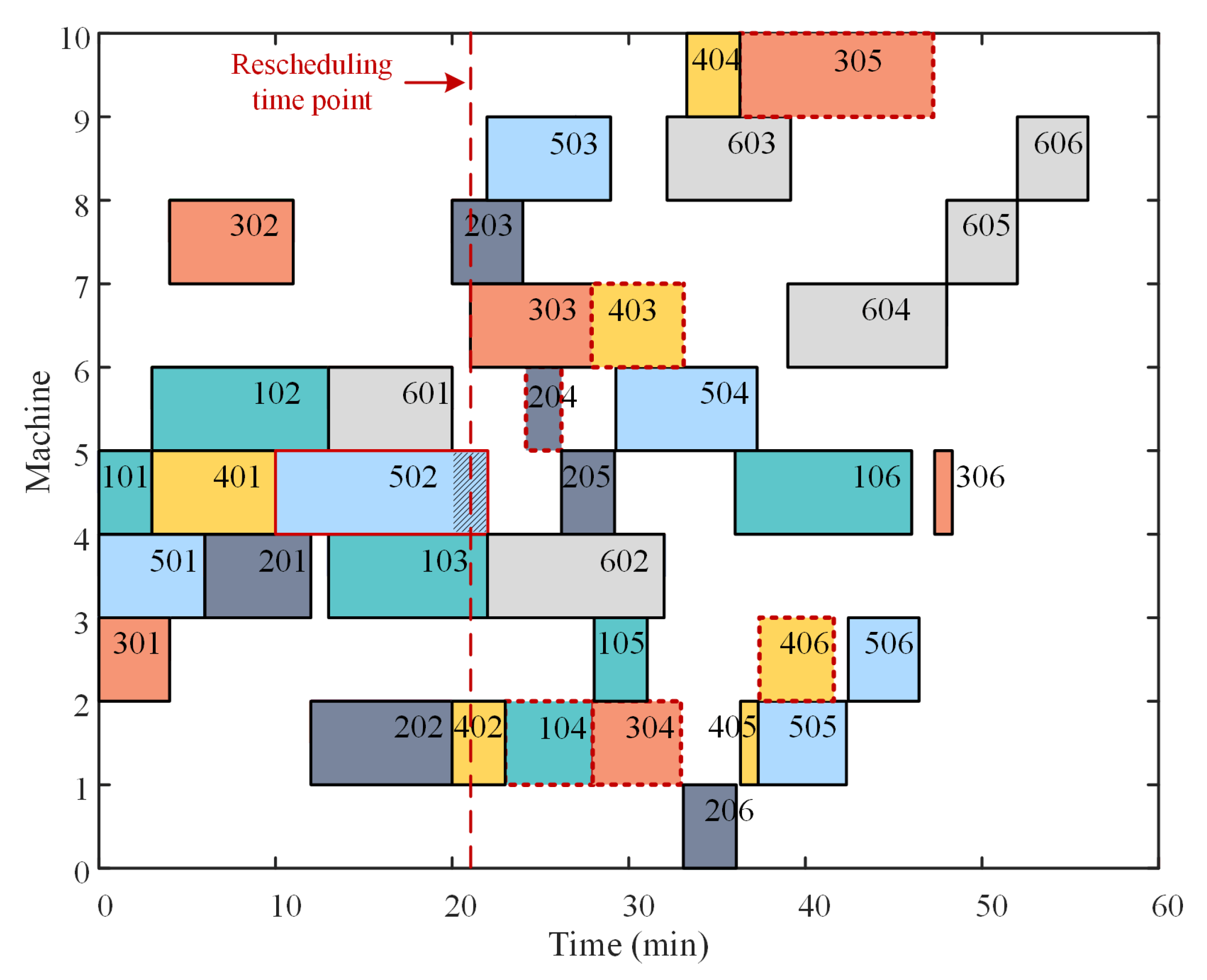
In the process of data collection, an important parameter (mean activity level of key branches) needs to be calculated based on the RSR scheme. As shown in Figure 5, the key branch is defined as the branch from a disturbed process to an overdue process. If one overdue process happens several times, the branch with the most compact time between processes and the preferential machine dimension influence will be selected. If the disturbance in process 201 leads to the overdue completion of processes 103 and 303, two key branches (201→302→103; 201→302→303) will occur.

For obtaining the key branches, the average activity level of the key branches is defined as follows:

$$ROM\_average=\frac{{{\displaystyle \sum }}_1^L{{\displaystyle \sum }}_1^{k}RO{M}_{l_k}}{L}$$

(3)

$$RO{M}_{l_k}=\{\left(C_{l_k}-1\right)/(C_{max}-1)\}\ast \delta$$

(4)

$$\delta =\{\begin{array}{c}0 , \mathrm{S}\mathrm{t}\mathrm{e}\mathrm{p} l_k \mathrm{c}\mathrm{a}\mathrm{n} \mathrm{n}\mathrm{o}\mathrm{t} \mathrm{b}\mathrm{e} \mathrm{c}\mathrm{o}\mathrm{m}\mathrm{p}\mathrm{l}\mathrm{e}\mathrm{t}\mathrm{e}\mathrm{d} \mathrm{a}\mathrm{h}\mathrm{e}\mathrm{a}\mathrm{d} \mathrm{o}\mathrm{f} \mathrm{t}\mathrm{i}\mathrm{m}\mathrm{e} \mathrm{o}\mathrm{n} \mathrm{o}\mathrm{t}\mathrm{h}\mathrm{e}\mathrm{r} \mathrm{o}\mathrm{p}\mathrm{t}\mathrm{i}\mathrm{o}\mathrm{n}\mathrm{a}\mathrm{l} \mathrm{m}\mathrm{a}\mathrm{c}\mathrm{h}\mathrm{i}\mathrm{n}\mathrm{e}\mathrm{s}\\ 1 ,\mathrm{S}\mathrm{t}\mathrm{e}\mathrm{p} l_k \mathrm{c}\mathrm{a}\mathrm{n} \mathrm{b}\mathrm{e} \mathrm{c}\mathrm{o}\mathrm{m}\mathrm{p}\mathrm{l}\mathrm{e}\mathrm{t}\mathrm{e}\mathrm{d} \mathrm{a}\mathrm{h}\mathrm{e}\mathrm{a}\mathrm{d} \mathrm{o}\mathrm{f} \mathrm{s}\mathrm{c}\mathrm{h}\mathrm{e}\mathrm{d}\mathrm{u}\mathrm{l}\mathrm{e} \mathrm{o}\mathrm{n} \mathrm{o}\mathrm{t}\mathrm{h}\mathrm{e}\mathrm{r} \mathrm{o}\mathrm{p}\mathrm{t}\mathrm{i}\mathrm{o}\mathrm{n}\mathrm{a}\mathrm{l} \mathrm{m}\mathrm{a}\mathrm{c}\mathrm{h}\mathrm{i}\mathrm{n}\mathrm{e}\mathrm{s}\end{array}$$

(5)

Formula (3) indicates some information in the key branch process set. $ROM\_average$ is the average activity level of the key branch, $RO{M}_{l_k}$ is the activity level of the $l_k$ process, and $L$ is the number of the key branches. Formula (4) represents the activity level of $l_k$, which is the process $k$ of the branch $l$. $C_{l_k}$ represents the number of selectable machining machines in the process $l_k$, and $C_{max}$ represents the maximum number of selectable machining machines in all the processes.

After data collection, duplicate samples and abnormal samples need to be deleted. For the abnormal samples, the data belonging to RSR will not appear for individuals whose average activity level of key branches is greater than 0. However, during the optimization process, the algorithm could find itself in a local optimal condition. Therefore, these samples should be deleted.

The next step is feature selection. Since most of the collected data have a nonlinear relationship with the decision label, the Spearman Correlation Coefficient [38] is used to analyze the data correlation, and then the feature vector with a correlation coefficient less than 0.1 is deleted. The feature vector finally selected is shown in

Table 3. Feature vectors and correlation coefficients.

Feature vector	①	②	③	④	⑤
Correlation coefficient	0.1282	0.2420	0.2532	−0.2748	0.1032
Feature vector	⑥	⑦	⑧	⑨	⑩
Correlation coefficient	0.2487	0.3682	0.2532	0.2420	0.3719

:

The feature vectors from 1 to 10 are as follows: ① the value beyond the time point of the processing end time of the disturbed procedure; ② the number of unprocessed procedures; ③ the number of affected procedures; ④ whether the disturbed procedure and overdue procedure are the same as the workpiece; ⑤ the load rate; ⑥ the total remaining processing time; ⑦ the total remaining idle time; ⑧ the proportion of PR procedures; ⑨ the proportion of TR procedures; and ⑩ the average activity level of key branches.

It is important to explain the decision label in addition to the feature vectors mentioned previously. There are three kinds of prediction results: RSR, PR, and TR, which are represented by labels “a”, “b”, and “c”, respectively, just as shown in Formula (2).

3.4. Model Training and Algorithm Optimization

Finally, the processed data are input into the model training and optimization module to train the machine learning model. When the rescheduling needs to be carried out in actual production, the disturbance data are input into the trained model, and the rescheduling selection decision is output. Model training and algorithm optimization are described in the next chapter.

4. Improved Whale Optimization Algorithm to Optimize Support Vector Machine

The goal of the support vector machine (SVM), which is widely used in classification regression problems, is to obtain the best classification regression effect with limited data information. It is crucial to determine the proper SVM parameters in enhancing prediction accuracy. Many researchers use optimization algorithms to optimize parameters. However, the majority of conventional optimization techniques suffer from sluggish convergence and are susceptible to local optimality [39]. Therefore, this paper selects the whale optimization algorithm with good performance in both global and local searches to determine the SVM parameters [40]. Additionally, the initial search range of the whale optimization algorithm (WOA) is then optimized on this basis to make its search efficiency higher.

4.1. Whale Optimization Algorithm

The Whale Optimization Algorithm (WOA) [41], proposed by Mirjalili and Lewis in 2016, is a meta-heuristic algorithm. WOA is a swarm intelligence optimization algorithm that simulates the social behavior of humpback whales in the hunting process. It hunts by encircling prey, searching for prey, and doing a spiral trajectory search.

(1)

Encircling prey

When $\left|A\right|<1$, the position update formula can be expressed:

$$D=|E·X^{*}\left(t\right)-X\left(t\right)|$$

(6)

$$X\left(t+1\right)=X^{*}\left(t\right)-A·D$$

(7)

where $D$ represents the distance from the whale to prey, $X$ represents the position of the current individual whale, $X^{*}$ represents the best individual whale, $t$ represents the number of iterations, and $A$ and $E$ are coefficient vectors:

$$A=2a·r-a$$

(8)

$$E=2r ,r\in \left[0,1\right]$$

(9)

where $r$ is the random number in the range, and $a$ decreases linearly from 2 to 0 in the iteration process.

(2)

Search for prey

When $\left|A\right|\ge 1$, the position update formula can be expressed as follows:

$$D=|E·X_{rand}-X\left(t\right)|$$

(10)

$$X\left(t+1\right)=X_{rand}-A·D$$

(11)

where $X_{rand}$ represents random whale individuals. When $\left|A\right|\ge 1$, it is selected as the optimal individual to update the location of other individuals.

(3)

Spiral trajectory search

The formula of motion trajectory can be calculated as follows:

$$D^{\prime }=|X^{*}\left(t\right)-X\left(t\right)|$$

(12)

$$X\left(t+1\right)=X^{*}\left(t\right)+D·e^{b·l}·\cos 2\pi l$$

(13)

where $b$ is the constant to define the shape of the logarithmic helix and $l$ is the random number between [−1, 1].

4.2. Support Vector Machine

Support vector machine (SVM) is a new classification algorithm developed on the basis of statistical learning proposed by Aljarah I [42], which has the advantages of fewer training samples, short time, and high precision. It is originally designed to solve binary classification problems, and its classification idea is to make the maximum interval between two separate categories as far as possible. On the basis of binary classification, the SVM classification method of multiple categories is developed.

SVM binary classification needs to find a linear function to determine the hyperplane. The linear function can be shown as follows:

$$y={\omega }^T·x+b$$

(14)

where $\omega$ is the coefficient vector and $b$ is the offset vector. Formula (14) can be converted to a convex quadratic programming optimization problem:

$$minJ\left(\omega ,\mathsf{\xi }\right)=\frac{1}{2}|\omega {|}^2+C{{\displaystyle \sum }}_{i=1}^n{\mathsf{\xi }}_i$$

(15)

$$s.t.\{\begin{array}{c}{y}_i\left({\omega }^T·x_i+b\right)\ge 1-{\mathsf{\xi }}_i\\ {\mathsf{\xi }}_i\ge 0, i=1,2,\dots ,n\end{array}$$

(16)

In Formula (15), ${\mathsf{\xi }}_i$ is the relaxation vector; $C$ is the penalty parameter; the Lagrange multiplier is introduced in Formula (17), which transforms the problem into a dual problem. It can be represented by the following:

$$maxW\left(\alpha \right)={{\displaystyle \sum }}_{i=1}^n{\alpha }_i-\frac{1}{2}{{\displaystyle \sum }}_{i=1}^n{{\displaystyle \sum }}_{j=1}^n{\alpha }_i{\alpha }_j{y}_i{y}_{j}k\left(x_i,x_j\right)$$

(17)

$$s.t.\{\begin{array}{c}{\displaystyle \sum }_{i=1}^n{\alpha }_i{y}_i=0\\ c>{\alpha }_i>0\end{array}i=1,2,\dots ,n$$

(18)

where $k\left(x_i,x_j\right)$ is the kernel function and ${\alpha }_i$ is a Lagrange multiplier. Based on Formulas (17) and (18), the classification model is obtained as follows:

$$f\left(x\right)=\mathrm{sgn}\left({{\displaystyle \sum }}_{i=1}^n{\alpha }_i{y}_{i}k\left(x_i,x_j\right)+b\right)$$

(19)

In this paper, the formula with RBF kernel function is as follows:

$$k\left(x_i,x_j\right)=\exp \left(-\Vert x_i-x_j{\Vert }^2/g^2\right)$$

(20)

where $g$ is the kernel parameter.

4.3. Improved WOA to Optimize SVM Parameters

The penalty parameter $C$ and the kernel parameter $g$ are two important parameters that affect the classification accuracy of the SVM. Through the use of an optimization method, a better parameter combination must be found. This paper improves the WOA-SVM in finding better parameters. Figure 6 expresses the flow of reducing parameter range.

The flow of determining the range of parameters $C$ and $g$ is as follows:

Step 1: Normalize the data in the data set and randomly extract the data set.

A total of 80% is the training set and 20% is the test set.

Step 2: Narrow the range of parameters $C$ and $g$. As shown in Figure 6, the range of initial parameters $C$ and $g$ is divided into $z$ segments within their respective ranges, and the breakpoint of each segment is tested for prediction accuracy. Then, collect the data and information of each breakpoint, select the best breakpoints according to a reasonable proportion, and then select the corresponding parameter range.

Step 3: Receive the range of parameters $C$ and $g$, and initialize the population and location.

Step 4: Perform parameter optimization by WOA and cross validation.

Step 5: Calculate the fitness function to determine whether the termination condition is met.

Step 6: Update the current optimal solution.

Step 7: Output the optimal solution.

5. Experiment

5.1. Single Sample Example

In order to confirm the effectiveness of the machine learning method in rescheduling decision problems, we undertook a single sample experiment. In the experiment, 6 workpieces are processed on 10 machines, and each workpiece needs to be processed for 6 processes. The optional processing machines and processing time are shown in

Table 4. Optional machining machines for the process.

	Process 1	Process 2	Process 3	Process 4	Process 5	Process 6
Workpiece 1	5	6	4	[2, 9]	[3, 7]	5
Workpiece 2	4	[2, 9]	8	[6, 7]	5	[1, 10]
Workpiece 3	3	[6, 8]	7	[2, 1]	[4, 10]	5
Workpiece 4	5	2	[4, 7]	[3, 10]	[2, 5]	[3, 6]
Workpiece 5	[4, 5]	5	[9, 10]	6	2	[3, 8]
Workpiece 6	[2, 6]	4	[6, 9]	7	8	[3, 9]

and

Table 5. Schedule of processing time.

	Process 1	Process 2	Process 3	Process 4	Process 5	Process 6
Workpiece 1	3	10	9	[5, 4]	[3, 3]	10
Workpiece 2	6	[8, 6]	4	[2, 6]	3	[3, 3]
Workpiece 3	4	[5, 7]	7	[5, 5]	[9, 11]	1
Workpiece 4	7	3	[4, 6]	[3, 3]	[1, 7]	[3, 6]
Workpiece 5	[6, 4]	10	[7, 9]	8	5	[4, 7]
Workpiece 6	[3, 7]	10	[8, 7]	9	4	[9, 4]

.

Firstly, genetic algorithm (GA) was used to obtain the original scheduling scheme [43,44], and the processing state and makespan data of each process could be obtained, as shown in Figure 7. Figure 8 shows the RSR scheme. If there is a disturbance in process 502 and the disturbance time is 1.8 min, many processes, such as 503, 104, and 603, are delayed, while it is assumed that the original delivery time of workpiece NO.6 is at time point 56 min. So, the rescheduling time point of process 502 is deduced to 21 min. The final delivery time of workpiece NO.6 is put off until 56.8 min after disturbance. RSR is, therefore, inappropriate in this scenario.

Figure 9 shows the PR scheme, and the delivery time of workpiece NO.6 is still 56 min. Only processes 503 and 104 are moved to other machines after disturbance occurring in process 502. PR does not significantly alter the original scheduling scheme.

Figure 10 shows the TR scheme, and the delivery time of workpiece NO.6 is still 56 min. It can be seen that there are much more processes that have changed the processing machine, compared with PR scheme. Therefore, the TR scheme changes the original scheme very much and wastes a lot of manpower and resources.

In summary, 10 feature vectors are obtained from the three rescheduling methods, as shown in

Table 6. Feature vector data table.

The Exceedance of the End Time of the Disturbed Operation	0.80 min
Number of unprocessed processes	23
Number of processes affected	16
Whether the disturbance process and overdue process are the same as the workpiece	0
Load rate	0.6043
Total remaining processing time	129.80 min
Total free time	85.00 min
Proportion of PR process	0.4444
Proportion of TR process	0.6389
Average activity level of key branches	1
Makespan of RSR (label 1)	56.80 min
Makespan of PR (label 2)	56.00 min
Makespan of TR (label 3)	56.00 min
Decision label	b

. By contrasting the three schemes, “b”, or the PR scheme, is the final decision label.

5.2. Large Sample Data Collection

According to the method of single sample data collection, repeat many times to obtain large sample data set. The operation steps are as follows:

Step 1: Delete duplicate values. Deduplication is performed on 30,000 samples data, and the number of samples after deletion is 27,603.

Step 2: Delete outliers. Filter the samples after deleting duplicate values. There are 1347 abnormal samples labeled “a” with the average activity of key branches greater than 0, and the probability of abnormal data is 4.88%. The number of samples is 26,256 after deletion.

Step 3: Sample distribution. The 26,256 groups of data retained are analyzed, as shown in Figure 11. The abscissa is the process number, and the ordinate is the sample size. A total of 36 processes from 101 to 606 are numbered on the horizontal coordinate.

Among 26,256 groups of sample data, the number of samples with decision label “a” is 14719, accounting for 56.06%. The number of samples whose decision label is “b” is 3422, accounting for 13.03%. The number of samples with decision label “c” is 8115, accounting for 30.91%.

5.3. Machine Learning Contrast Test

To test the accuracy of machine learning under different sample sizes. There are 300 groups, 900 groups, 1800 groups, 3000 groups, and 6000 groups of data being predicted through different machine learning ways. The sample size of three rescheduling schemes is same. Taking the test of 6000 data sets as an example, parameters $C$ and $g$ are divided into 100 breaks, respectively, and the accuracy of each breakpoint is calculated. The relationship between parameters $C$, $g$, and the prediction accuracy is shown in Figure 12.

According to the statistical data and Figure 13, the distribution with the highest accuracy is in the range of parameter $C$ [0.00001, 10] and parameter $g$ [0.00001, 1000], which are also the two-parameter search range of WOA. WOA is used to find the optimal parameter values in this range. Then, the parameters are input into SVM to train the model. A total of 80% of the data are used as the training set. A total of 20% of the data are used as the test set. Predictions of different data scales are tested 100 times, and the average accuracy is shown in

Table 7. Accuracy Rate.

Machine Learning Techniques	Scale of Data
	300	900	1800	3000	6000
WOA-SVM	70.08%	75.57%	80.35%	83.46%	89.79%
SVM(RBF)	71.41%	71.24%	71.88%	72.56%	70.01%
BP	71.95%	74.33%	73.99%	75.29%	71.94%

.

As can be seen from Table 7, the prediction accuracy of the WOA-SVM increases with the growth in sample size. Its prediction accuracy is low when the sample size is small. The reason is that the algorithm falls into local optimality. To show the frequency of this problem, Pauta criteria [45] are used to check abnormal data. The frequency of abnormal data is shown in

Table 8. Abnormal rates.

Machine Learning Techniques	Scale of Data
	300	900	1800	3000	6000
WOA-SVM	1%	34%	27%	5%	0%
SVM(RBF)	8%	6%	8%	4%	5%
BP	14%	6%	3%	4%	0%

.

In Table 8, the frequency of abnormal data decreases with the increase in sample size in general. The abnormal frequency of 6000 groups in the WOA-SVM has gone down to 0%. At this time, the prediction accuracy also reached the highest (89.79% in Table 7). In

Table 9. Confusion matrix.

	Predictive Classification			Aggregate	Accuracy Rate
	RSR	PR	TR
RSR	351	14	35	400	87.75%
PR	18	366	16	400	91.50%
TR	11	29	360	400	90.00%
Aggregate	380	409	411	1200

, The total number of samples in the test set is 1200, with 400 samples for each of the three categories. The number of samples with correct prediction in RSR is 351. The number of samples with correct prediction in PR is 366. The number of samples with correct prediction in TR is 360. It can be seen that the prediction accuracy in the RSR sample is the lowest, only 87.85%. In the other two samples, the prediction accuracy is relatively high, resulting in an overall prediction accuracy of 89.79%.

The accuracy of 100 tests in 6000 groups is summarized in Figure 13. The abscissa is the number of the experiment. The ordinate represents prediction accuracy. Obviously, the accuracy of BP and SVM are between 64% and 76% and have large swing ranges, while the accuracy of the WOA-SVM stays around 89%, and the fluctuation is no more than 1%. So, the WOA-SVM method is superior to SVM and BP methods in terms of prediction accuracy and stability.

6. Conclusions

For the various disturbances in the flexible job shop, a rescheduling schedule is constructed by analysis of the dynamic correlation among processes, and the time point of rescheduling is specified at each process. This method can be used to solve the problem of unclear rescheduling boundaries when disturbances occur in the actual production.

A decision method of rescheduling mode based on machine learning is proposed. Experimental results show that machine learning technology has higher accuracy in the decision of flexible job shop rescheduling mode, compared with the traditional decision mode by personnel experience. It means that the decision method by machine learning can better meet the requirements of intelligent patterns, precision, and high efficiency in modern manufacturing enterprises. The improved WOA-SVM mothed is used to predict some randomly generated data samples. It is proved that the WOA-SVM has a good performance in prediction accuracy and prediction stability compared to other prediction methods.

References

1. Jin, P.; Tang, Q.; Cheng, L.; Zhang, L. Decision-Making Model of Production Rescheduling Mode for Flexible Job Shops under Machine Failures. Comput. Integr. Manuf. Syst. 1–13. Available online: http://kns.cnki.net/kcms/detail/11.5946.tp.20211006.0811.002.html (accessed on 17 January 2023).
2. Dai, M.; Tang, D.; Giret, A.; Salido, M.A. Multi-objective optimization for energy-efficient flexible job shop scheduling problem with transportation constraints. Robot. Comput. Integr. Manuf. 2019, 59, 143–157. [Google Scholar] [CrossRef]
3. Zhang, F.; Mei, Y.; Nguyen, S.; Zhang, M. Collaborative multifidelity-based surrogate models for genetic programming in dynamic flexible job shop scheduling. IEEE Trans. Cybern. 2021, 52, 8142–8156. [Google Scholar] [CrossRef] [PubMed]
4. Liu, S.C.; Chen, Z.G.; Zhan, Z.H.; Jeon, S.W.; Kwong, S.; Zhang, J. Many-objective job-shop scheduling: A multiple populations for multiple objectives-based genetic algorithm approach. IEEE Trans. Cybern. 2021, 1–15. [Google Scholar] [CrossRef] [PubMed]
5. Yan, J.; Liu, Z.; Zhang, C.; Zhang, T.; Zhang, Y.; Yang, C. Research on flexible job shop scheduling under finite transportation conditions for digital twin workshop. Robot. Comput. Integr. Manuf. 2021, 72, 102198. [Google Scholar] [CrossRef]
6. Kacem, I.; Hammadi, S.; Borne, P. Approach by localization and genetic manipulation algorithm for flexible job-shop scheduling problem. In Proceedings of the 2001 IEEE International Conference on Systems, Man and Cybernetics, e-Systems and e-Man for Cybernetics in Cyberspace (Cat. No. 01CH37236), IEEE, Tuscon, AZ, USA, 7–10 October 2001; Volume 4, pp. 2599–2604. [Google Scholar]
7. Kacem, I.; Hammadi, S.; Borne, P. Approach by localization and multi-objective evolutionary optimization for flexible job-shop scheduling problems. IEEE Trans. Syst. Man Cybern. Part C (Appl. Rev.) 2002, 32, 1–13. [Google Scholar] [CrossRef]
8. Wu, X.; Sun, S.; Yu, J.; Zhang, H. Research on multi-objective for flexible job shop scheduling. Comput. Integr. Manuf. Syst. 2006, 5, 731–736. [Google Scholar]
9. Yu, J.; Sun, S.; Hao, J. Multi objective flexible job-shop scheduling based on immune algorithm. Comput. Integr. Manuf. Syst. 2006, 12, 1643. [Google Scholar]
10. Afsar, S.; Palacios, J.J.; Puente, J.; Vela, C.R.; González-Rodríguez, I. Multi-objective enhanced memetic algorithm for green job shop scheduling with uncertain times. Swarm Evol. Comput. 2022, 68, 101016. [Google Scholar] [CrossRef]
11. Alkhateeb, F.; Abed-alguni, B.H.; Al-rousan, M.H. Discrete hybrid cuckoo search and simulated annealing algorithm for solving the job shop scheduling problem. J. Supercomput. 2022, 78, 4799–4826. [Google Scholar] [CrossRef]
12. Caldeira, R.H.; Gnanavelbabu, A. A Pareto based discrete Jaya algorithm for multi-objective flexible job shop scheduling problem. Expert Syst. Appl. 2021, 170, 114567. [Google Scholar] [CrossRef]
13. Ibrahim, A.M.; Tawhid, M.A. An improved artificial algae algorithm integrated with differential evolution for job-shop scheduling problem. J. Intell. Manuf. 2022, 1–16. [Google Scholar] [CrossRef]
14. Brandimarte, P. Routing and scheduling in a flexible job shop by tabu search. Ann. Oper. Res. 1993, 41, 157–183. [Google Scholar] [CrossRef]
15. Baykasoğlu, A.; Madenoğlu, F.S.; Hamzadayı, A. Greedy randomized adaptive search for dynamic flexible job-shop scheduling. J. Manuf. Syst. 2020, 56, 425–451. [Google Scholar] [CrossRef]
16. Mohan, J.; Lanka, K.; Rao, A.N. A review of dynamic job shop scheduling techniques. Procedia Manuf. 2019, 30, 34–39. [Google Scholar] [CrossRef]
17. Priore, P.; De La Fuente, D.; Gomez, A.; Puente, J. A review of machine learning in dynamic scheduling of flexible manufacturing systems. Ai Edam 2001, 15, 251–263. [Google Scholar] [CrossRef]
18. Wang, L.; Hu, X.; Wang, Y.; Xu, S.; Ma, S.; Yang, K.; Liu, Z.; Wang, W. Dynamic job-shop scheduling in smart manufacturing using deep reinforcement learning. Comput. Netw. 2021, 190, 107969. [Google Scholar] [CrossRef]
19. Zhang, C.; Song, W.; Cao, Z.; Zhang, J.; Tan, P.S.; Chi, X. Learning to dispatch for job shop scheduling via deep reinforcement learning. Adv. Neural Inf. Process. Syst. 2020, 33, 1621–1632. [Google Scholar]
20. Chen, R.; Yang, B.; Li, S.; Wang, S. A self-learning genetic algorithm based on reinforcement learning for flexible job-shop scheduling problem. Comput. Ind. Eng. 2020, 149, 106778. [Google Scholar] [CrossRef]
21. Cao, X.; Ma, R.; Liu, L.; Shi, H.; Cheng, Y.; Sun, C. A machine learning-based algorithm for joint scheduling and power control in wireless networks. IEEE Internet Things J. 2018, 5, 4308–4318. [Google Scholar] [CrossRef]
22. Weckman, G.R.; Ganduri, C.V.; Koonce, D.A. A neural network job-shop scheduler. J. Intell. Manuf. 2008, 19, 191–201. [Google Scholar] [CrossRef]
23. Hameed, M.S.A.; Schwung, A. Reinforcement learning on job shop scheduling problems using graph networks. arXiv 2020, arXiv:2009.03836. [Google Scholar]
24. Fang, Y.; Peng, C.; Lou, P.; Zhou, Z.; Hu, J.; Yan, J. Digital-twin-based job shop scheduling toward smart manufacturing. IEEE Trans. Ind. Inform. 2019, 15, 6425–6435. [Google Scholar] [CrossRef]
25. Zhang, M.; Tao, F.; Nee, A.Y.C. Digital twin enhanced dynamic job-shop scheduling. J. Manuf. Syst. 2021, 58, 146–156. [Google Scholar] [CrossRef]
26. Tong, Z.; Deng, X.; Chen, H.; Mei, J.; Liu, H. QL-HEFT: A novel machine learning scheduling scheme base on cloud computing environment. Neural Comput. Appl. 2020, 32, 5553–5570. [Google Scholar] [CrossRef]
27. Morariu, C.; Morariu, O.; Răileanu, S.; Borangiu, T. Machine learning for predictive scheduling and resource allocation in large scale manufacturing systems. Comput. Ind. 2020, 120, 103244. [Google Scholar] [CrossRef]
28. Liu, D.; Zhu, G.; Zhang, J.; Huang, K. Data-importance aware user scheduling for communication-efficient edge machine learning. IEEE Trans. Cogn. Commun. Netw. 2020, 7, 265–278. [Google Scholar] [CrossRef]
29. Ghasemi, A.; Ashoori, A.; Heavey, C. Evolutionary learning based simulation optimization for stochastic job shop scheduling problems. Appl. Soft Comput. 2021, 106, 107309. [Google Scholar] [CrossRef]
30. Amiri, M.M.; Gündüz, D. Computation scheduling for distributed machine learning with straggling workers. IEEE Trans. Signal Process. 2019, 67, 6270–6284. [Google Scholar] [CrossRef] [Green Version]
31. Faraji, J.; Ketabi, A.; Hashemi-Dezaki, H.; Shafie-Khah, M.; Catalão, J.P. Optimal day-ahead self-scheduling and operation of prosumer microgrids using hybrid machine learning-based weather and load forecasting. IEEE Access 2020, 8, 157284–157305. [Google Scholar] [CrossRef]
32. Müller, D.; Müller, M.G.; Kress, D.; Pesch, E. An algorithm selection approach for the flexible job shop scheduling problem: Choosing constraint programming solvers through machine learning. Eur. J. Oper. Res. 2022, 302, 874–891. [Google Scholar] [CrossRef]
33. Jun, S.; Lee, S.; Chun, H. Learning dispatching rules using random forest in flexible job shop scheduling problems. Int. J. Prod. Res. 2019, 57, 3290–3310. [Google Scholar] [CrossRef]
34. Li, Z.C.; Qian, B.; Hu, R.; Chang, L.L.; Yang, J.B. An elitist nondominated sorting hybrid algorithm for multi-objective flexible job-shop scheduling problem with sequence-dependent setups. Knowl. Based Syst. 2019, 173, 83–112. [Google Scholar] [CrossRef]
35. Li, X.; Zuo, D. Two-phase genetic algorithm for multi-objective flexible job-shop scheduling problem. J. Comput. Appl. 2020, 40, 14–22. [Google Scholar]
36. Zhao, H. Research on Robust Scheduling of Manufacturing Enterprises under MTO Mode; Chongqing University of Technology: Chongqing, China, 2015. [Google Scholar]
37. Wang, W.; Ge, X.; Li, L.; Su, J. Proactive and reactive multi-project scheduling in uncertain environment. IEEE Access 2019, 7, 88986–88997. [Google Scholar] [CrossRef]
38. Myers, L.; Sirois, M.J. Spearman correlation coefficients, differences between. Encycl. Stat. Sci. 2004, 12, 1–3. [Google Scholar]
39. Baxter, J. Local optima avoidance in depot location. J. Oper. Res. Soc. 1981, 32, 815–819. [Google Scholar] [CrossRef]
40. Nguyen, H.; Bui, X.N.; Choi, Y.; Lee, C.W.; Armaghani, D.J. A novel combination of whale optimization algorithm and support vector machine with different kernel functions for prediction of blasting-induced fly-rock in quarry mines. Nat. Resour. Res. 2021, 30, 191–207. [Google Scholar] [CrossRef]
41. Mirjalili, S.; Lewis, A. The whale optimization algorithm. Adv. Eng. Softw. 2016, 95, 51–67. [Google Scholar] [CrossRef]
42. Aljarah, I.; Al-Zoubi, A.M.; Faris, H.; Hassonah, M.A.; Mirjalili, S.; Saadeh, H. Simultaneous feature selection and support vector machine optimization using the grasshopper optimization algorithm. Cogn. Comput. 2018, 10, 478–495. [Google Scholar] [CrossRef] [Green Version]
43. Zhao, Z.Y.; Yuan, Q.L. Integrated Multi-objective Optimization of Predictive Maintenance and Production Scheduling: Perspective from Lead Time Constraints. J. Intell. Manag. Decis. 2022, 1, 67–77. [Google Scholar] [CrossRef]
44. Badi, I.; Jibril, L.; Bakır, M. A Composite Approach for Site Optimization of Fire Stations. J. Intell. Manag. Decis. 2022, 1, 28–35. [Google Scholar] [CrossRef]
45. Xu, C.; Ma, M. Optimization Method for Gross Error Processing of Traffic Data Based on Pauta Criterion. J. Shanghai Univ. Eng. Sci. 2018, 32, 64–67. [Google Scholar]
Figure 1. Original scheduling scheme.
Systems 11 00059 g001
Figure 2. Rescheduling mode selection framework.
Systems 11 00059 g002
Figure 3. Correlation among processes.
Systems 11 00059 g003
Figure 4. Rescheduling time point determination.
Systems 11 00059 g004
Figure 5. Key branches.
Systems 11 00059 g005
Figure 6. Flow chart of WOA-SVM parameters.
Systems 11 00059 g006
Figure 7. Original scheduling scheme.
Systems 11 00059 g007
Figure 8. RSR scheme.
Systems 11 00059 g008
Figure 9. PR scheme.
Systems 11 00059 g009
Figure 10. TR scheme.
Systems 11 00059 g010
Figure 11. Sample distribution.
Systems 11 00059 g011
Figure 12. Parameter C , g –Prediction accuracy.
Systems 11 00059 g012
Figure 13. Comparison of test accuracy of 6000 groups of data.
Systems 11 00059 g013