1. Introduction
Agent-based modeling (ABM) is increasingly popular [
1]: more powerful computation technologies, and an increasing interest in simulating complex social systems, have led to a surge in such models. The approach is applied ubiquitously—from problems as imminent as pandemics [
2] to abstract-use cases, such as modeling cardio-vascular systems [
3].
A common understanding of ABM is that individual entities (agents) moving in and independently acting upon a dynamic environment are the constituents of such a model [
4]. Methodologically, these models are primarily implemented as rule-based models [
5]. The agents follow certain rules set by the modeler [
6]: such models starkly contrast with equation-based models, which rely on differential equations to describe their behavior [
1,
7,
8]. The idea behind rule-based modeling is to provide an algorithmic description of the attributed behavior [
5]. In many cases of social simulation, this attributed behavior is targeted at simulating intelligent decision making: such intelligent agents are considered the pinnacle of ABM by some scholars [
9].
While the individual decisions of agents are driven by the rules imposed by the author of the model, collective intelligent behavior can arise from the model itself—similarly to, for example, colonies of bacteria: an individual bacterium is clearly unconscious; however, when collected in colonies, bacteria appear to conduct intelligent activities, such as competing, working together to search for food, and exchanging chemical and physical signals between cells [
10].
However, compressing intelligent decisions into a set of rules has been shown to cause shortcomings [
11]: every behavior that is to be described requires a tailored rule [
6]; the set of rules is often inadvertently biased [
11]; rule-based agents are limited in their ability to learn from their environment and adapt to changing conditions; rules can be too rigid to capture more complex behaviors and interactions; and rule-based agents are limited in their capacity to represent uncertainty and stochasticity. Some of these limitations can be mitigated, for example, by adding probability-based rules [
12,
13].
To capture the complexity of real-world behavior, the concept of bounded rationality is often used in ABMs, especially when focused on the economic behavior of agents [
14]. Bounded rationality is used to account for the limited cognitive abilities of individual agents, such as their limited information processing capacity and their limited ability to learn from experience [
15]. It is assumed that agents have a limited set of strategies (rules) that they can use to make decisions, and that they are unable to maximize their utility in all circumstances: this can lead to sub-optimal decisions and behaviors.
Generally speaking, the less bounded the thinking of an agent is, the more intelligent it can be considered, i.e., “agents with higher intelligence have lower bound of rationality” [
12]; however, when agents are designed to model human behavior realistically, they should be necessarily boundedly rational [
16]. Bounded rationality can be measured by examining the decision making process of an intelligent agent, often in an experimental setting [
17,
18]: this includes looking at the strategies and tactics used, the time taken to make decisions and the degree of success achieved, e.g., measured by the accuracy of predictions. However, there is no agreed-upon quantitative measure of the bounded rationality of agents in ABMs: one of the possible options is to measure agents’ knowledge [
12]. Bounded rationality in ABMs can, however, be explicitly introduced: for example, by varying the percentages of random noise in the decision function [
19].
Recently, the idea of incorporating more refined algorithms has gained traction [
20,
21,
22,
23]. The past decade has brought about vast advances in the field of artificial intelligence (AI): ABM is often considered a part of this field [
24], and it is, therefore, reasonable to consider other advances within this field as possible remedies for a lack of simulated intelligence in the agents.
Machine learning algorithms have gained popularity in many research areas: as such, they have also been incorporated in ABM, to achieve artificial intelligence in agents [
20,
22,
23]. At the same time, the concept of bounded rationality is still rarely used in AI studies [
16].
Artificial neural networks (ANNs) are capable of simulating behavior that is too complicated to be described in a reasonable set of rules. The behavior of ANNs can be fitted to existing data, yielding a representative behavior of the agents themselves [
20]; however, such algorithms are essentially black boxes, and are prone to overfitting [
25,
26]. ANNs may exhibit the same result with vastly varying parameters: in some areas, it could be more favorable to have an algorithm with better interpretability. One approach to this is to limit the number of input–output relations of ANNs, and to provide clear meaning to them, with fuzzy cognitive maps (FCMs) [
22,
27]. In contrast to ANNs and FCMs—both of which are essentially systems of linearly connected rules—another solution could be “one rule to rule them all”.
The behavior of systems ranging from cosmological [
28] to biological domains [
29] has recently been described using a single, fundamental, entropy-based formalism [
30]: similar advances in AI research have incorporated this mechanism as an approach to approximating intelligence in known environments [
30,
31,
32]. These methods have been summarized under the term “future state maximization” (FSX) [
33].
Research on FSX has mostly explored the astonishing cooperation emerging among swarms of agents equipped with such decision mechanics [
30,
31,
32,
34]. Behavior in ABM, however, should be capable of depicting interaction beyond beneficial effects for all entities [
35,
36]. In order to examine whether FSX can substitute traditional rule-based ABM, we need to show the boundaries of this emergent cooperation.
This leads us to our research question: can FSX yield an interpretable model of intelligent decision making, ranging from rational to irrational behavior?
After a literature review outlined in
Section 2, we will introduce FSX and our methodological approach in
Section 3. The results are presented in
Section 4, and are further discussed in
Section 5. The manuscript concludes with
Section 6, which outlines possible future developments.
2. Literature Review
The connection to entropy-based advances in other fields was mostly established by [
30], whose causal entropic forcing (CEF) exhibited the first-ever successful accomplishment of the string-pull test by artificial intelligence [
30]. Ref. [
30] sparked more in-depth research into the matter: in effect, CEF was used to simulate the forming of columns of people in a narrow passageway, and the flocking of birds [
32,
37]. Ref. [
34] expanded their research into a more detailed analysis of interactions within CEF-directed entities.
A similar approach to CEF was taken by [
31], who were more focused on the computational part, in what they introduced as fractal-AI. Somewhat earlier, [
38] pioneered the idea of CEF with their empowerment prospect: herein, an agent, rather than maximizing the entropy of its state, aimed at maximizing its control over said state [
38].
While there are some significant differences between causal entropic forcing, fractal-AI, and the empowerment theory, they still share a common principle, which can be subsumed into Heinz von Foerster’s ethical imperative [
33]:
“Act always so as to increase the number of choices”—[
39]
It is this notion that aids the interpretability of the agent’s behavior. Ref. [
32] embraced future state maximization (FSX) as an umbrella term for this general idea. We shall use this term as an understanding of an agent that aims to enlarge its space of possible future states. A closer explanation of the principle can be found in
Section 3.
Microscopic Traffic Modeling as Boundary Object
To answer our research question about the rationality-to-irrationality range of FSX, a support model was necessary: we found that microscopic traffic modeling presented a fitting boundary object for such a pilot study. Traffic situations can range from seemingly rational modest driving to irrational and selfish behavior [
40]: our aim was to explore the emergence of either situation, and the space in between, within a single framework.
In the realm of traffic modeling, agent-based models continue to gain in popularity [
41]. Common models employ a car-following approach, where an agent reacts to a car in front of it according to equations [
42,
43]. Some car-following models are coupled with a lane-changing model, to accommodate multiple road lanes [
42,
44]. However, popular models only cover perfect driving behavior, disregarding any misbehavior found in actual human driving [
42,
45]: there is a need to incorporate the irrational and unpredictable behavior of (human) agents [
40,
46]. Current car-following models are also lacking in their depiction of the vast heterogeneity of driving behaviors [
43].
Microscopic traffic scenarios range from cooperative to competitive behavior [
42,
44]: recently, there have been attempts to develop a model exposing both phenomena within one framework [
42]. Employing findings from psychology, one can achieve agent misbehavior similar to human actions in traffic situations [
42,
45]: however, these models are still rule-based, with the misbehavior being determined by the modeler a priori. Perhaps, as a result, current car-following models are not generalizable [
43].
Note, on the other hand, that FSX as a method is applicable to any agent-based model. A stylized ABM applied to microscopic traffic situations, as developed in this paper, merely serves as a supporting example, which allows us to explore a range of behaviors, from rational to irrational decision making. The two-dimensional nature of such a model facilitates investigation, e.g., future states of the agents are actual trajectories in 2D space and, thus, easy to visualize. The continuous decision space of our model, and the uncertain behavior of other agents, increases the complexity of the model, such that knowledge transfer to other ABMs becomes reasonable.
3. Method
Future state maximization embodies a common principle found in multiple, rather novel, research items [
30,
31,
32,
34]. To the best of our knowledge, no comparison exists of the various implementations published to date: however, all of them exhibit somewhat intelligent agents [
33].
Formalisms from research on causal entropic forcing (CEF) focus on the calculation of state entropy [
30,
34]. Ref. [
32] were the first to focus on the actual states: their agents scanned the entire future state space up to a horizon
. It is acknowledged that this works for a small
in a discrete state space, but is less applicable to continuous scenarios [
32]. The appended continuous method relies on a distance measure between states [
32]. By contrast, the algorithm of fractal-AI is applicable to continuous cases, without such a distance measure [
31].
The agents in [
31] made use of so-called “walkers”, which can be interpreted as particle representations of thought processes, i.e., virtual entities sent out to explore the future state space of an agent through a random walk [
31,
33,
34]. Ref. [
31] combined this idea of walkers with a mechanism for their (re-)distribution: thus, in contrast to CEF [
30], it features the ability to introduce a utility function [
31]. What had previously been a method to sample the future state space of the agent [
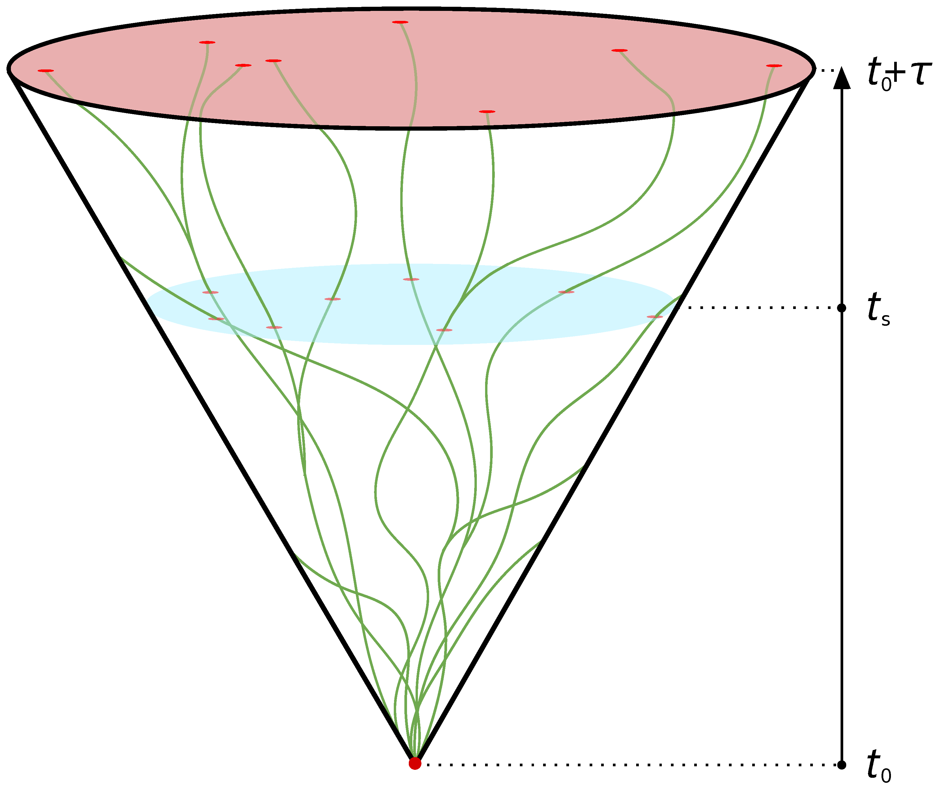
34], also referred to as its causal cone (see
Figure 1), was put into focus by [
31].
Walkers are created for each decision an agent faces. The walkers initially reside in the very state of the agent they are spawned from; consequently, according to fractal-AI [
31], each walker draws and performs one random action
from the agent’s action space. The action space can be either discrete or continuous. Each initial action is stored, together with the identity of the walker performing it, as a crucial part of the walker’s integrity [
31]. Note that each walker now finds itself in a new state,
, where
f is some simulation function, which need not be perfect (i.e., need not represent actual future development perfectly) nor deterministic [
31].
This state can now be evaluated via an evaluation function, which maps the state space to the binary result of “dead” or “alive”: for example, an agent could maintain a health bar similar to role-play games; then, the function would yield “dead” in the event that the health bar reached
, and “alive” otherwise. Dead walkers are not abandoned, but re-initiated. For each walker that vanishes, a random living walker is cloned, yielding two walkers with an identical initial choice and walker state [
31]. Each walker draws another, individual, random action, and the process repeats. Similar to CEF, the iterative process ends at the so-called horizon
. The walkers ultimately execute action
, and reach their final walker states [
30,
31,
34].
This can be followed through in
Figure 1, where an agent at
spawns 8 walkers. Note that, once the walkers (depicted as green strings) hit the edge of the cone, and thus cease to exist, another, living, walker is cloned. In effect, even though the walkers collide with the boundary in the process, the algorithm ensures that the number of walkers stays constant.
As a result, the distribution of the walkers approximates the distribution of the survivable future states of the agent that can be reached within the horizon [
31]. In discrete action space, the consequent action of the agent is then the initial option taken by most walkers; in continuous action space, it is the average initial decision of all the walkers [
31].
A major advantage of the fractal-AI algorithm is the possibility of incorporating a utility function denoted as reward [
31]: this is accomplished by skewing the walker distribution, such that it aligns with the distribution of reward [
31]. The effective reward in any future state can only be known at the walker positions. Hence, somewhat in contrast to CEF, fractal-AI relies on a sufficient number of walkers to arrive at an appropriate scanning density: this shall become evident in the sensitivity analysis found in
Section 4.
As discussed above, previous studies on FSX and related concepts still vary considerably in their methodological approach. Among those studies, our approach was most inspired by [
31]: that is, we created agents that explored their future state space using walkers. These walkers were redistributed, according to a utility function, to drive the agents towards an overarching objective.
3.1. Modeling the Environment and Its Development
The notion of the state of an agent relies on the environment it resides in. The environment used in this study was based on an infinite, two-dimensional, Cartesian coordinate system: within these coordinates, areas exist which can be understood to be accessible by agents. Any area inaccessible to agents will render their walkers dead. Other agents are also considered to be inaccessible areas. Hence, the agents are motivated to stay within the bounds of the accessible areas, and clear of other agents.
As [
47] argue, any action taken, and thus any decision, sparks an infinite number of future possibilities. Therefore, it is paramount to distinguish two different ways for the environment to evolve:
The former resembles the intuitive case: every agent executes its decision, and consequently arrives at a new state in
; however, before execution, the decision has to be found. At this stage, the actual development of the environment is unknown. A virtual time step reveals an approximation of such a future state. In this sense, the FSX approach differs from non-anticipatory optimal control algorithms [
48], which explore the possible (admissible) future states space on the entire horizon, before the actual decision on where to move at all consequent time steps is made: necessarily, this incorporates an agent’s beliefs about future development. We only considered agents with equal beliefs: however, due to this distinction, it would prove trivial to introduce, for example, the belief that others will slow down if oneself does not.
3.1.1. An Actual Time Step
The movements of the agents were processed sequentially. Similarly to [
42], the decisions of the agent were whether to brake or accelerate, and where to steer. These decisions were then executed, such that all agents arrived at their respective actual states
. Every single agent thus spawned a number of walkers, which in turn performed virtual time steps through the estimated future state space.
3.1.2. A Virtual Time Step
Virtual time steps require an estimate for the dynamic development of future state space. Agents are not capable of introspecting the causal cones of any other agent: such a mechanism would lead to infinite circularity. The necessary consequence is to incorporate a prediction of agent movements [
49]: this is accomplished by assuming that agents pursue their recent trajectory. Thus, virtual state
can be found through the realized states
and
:
Any further virtual state is then found by extrapolating these trajectories:
These virtual time steps construct the environment scanned by the walker entities. The future states that a walker experiences may differ from the actual state space the agent ultimately encounters: hence, a virtual time step can be regarded as the expectations of an agent about future development.
3.2. Implementation of the Agents
The agents—stylized cars—were rectangles with a length and a width . Movement forwards and backwards was restricted by the respective limited speeds, and . A minimum absolute speed, , was required to turn in any direction; however, the vehicle turning radius was limited by . The pivot point for turning was set in the center of the rear end of the vehicle. Acceleration and deceleration were idealized as being linear, and were limited by and : the movement of the walkers was restricted equally.
All these parameters of movement were set to closely resemble the parameters of [
50]: they are listed in
Table 1.
To endow the agents with future state maximizing capability, three additional parameters for the decision making process had to be considered: the horizon
; the number of walkers
; and the urgency to reach the objective
(more details on the types of objectives are given below). While the parameters of movement, i.e., those listed in
Table 1, remained constant, these three parameters were the subject of investigation.
3.2.1. Driving Behavior
The driving behavior of the agents emerged from the limits set, and from their decision making process. The decision was composed of two objectives: (i) survival, i.e., avoiding collision with other agents or with the boundaries of the model environment; (ii) optimizing a reward function. In contrast to [
31], we refrained from a single reward function encoding survival and utility functionality: this rendered balancing and assessing the influence of each single objective more accessible.
Survival was the primary objective. The state variable encoding the survival of a walker was binary: it equaled 1 if the walker was alive, and 0 if it was dead. After each virtual time step, walkers intersecting or going beyond the boundary of the accessible area were marked as dead according to Equation (
3):
where
i was the index of an agent spawning the walker
w, and
was the extrapolated position of the agent
at virtual time
t. The boundary was given through
b, and
A took the area of the intersections. If the intersected area was zero, the walker remained alive.
Additionally, a reward was introduced, to motivate the agents to move. This reward function was defined as
, where
d was the distance of the walker’s position,
, relative to the position of the agent’s goal
:
To redistribute walkers according to reward density, ref. [
31] introduced a quantity called “virtual reward”,
. This normalized measure of individual reward enabled comparison among walkers [
31]:
where
was the density of the walkers in the vicinity of the state of walker
i, and
was the reward. To align the walker density with the reward density, the virtual reward was balanced among all the walkers [
31]: this was achieved via a randomized redistribution process.
Firstly, ref. [
31] approximated
, in order to spare computational demand, by finding the distance to another random walker:
In our case, of a Euclidean space, the distance function
was trivially chosen as Euclidean distance: ref. [
31] does not specify any properties that such a function has to fulfill. Then, normalization functions
and
were introduced:
where
was intended to be the mean of the distribution containing
x, and
its standard deviation. Finally,
could be calculated as:
Equation (
9) introduces an additional parameter
: this parameter is intended to balance exploitation versus exploration [
31]. The idea is that a high
increases the weight of the reward: hence, agents will increasingly strive for reward as
increases. With
, the entropy of the walkers is emphasized. Agents explore their environment, disregarding the areas with higher pay-offs.
Aligning the walker distribution with the reward distribution works similarly to Algorithm 1; however, in contrast to the survival objective, a probability
of a walker being substituted is introduced:
This probability again relies on a randomly drawn walker, j, where . A complete lack of virtual reward immediately renders a walker due to be substituted, whereas a superior virtual reward ensures its survival. In the case of an inferior virtual reward, a normalized difference in the virtual reward establishes the probability of the walker i to be substituted. This mechanism is outlined in Algorithm 2.
3.2.2. Decision Making
With the walker redistribution functions defined, the formulation of an agent’s thought process is straightforward. As our model operated in continuous state space, we will focus on the description of this specific case.
In Algorithms 1 and 2, upon the cloning of a walker, its initial action was also duplicated; therefore, the ultimate distribution of initial decisions was skewed towards walkers which (a) survived, and (b) achieved a high reward. The decision of the agent was the mean of the surviving walkers’ initial decisions. A detailed description of this decision mechanism is given in Algorithm 3.
| Algorithm 1: Walker redistribution step 1: survival as objective. |
| 1: walkersNew ← Set() | ▹ Collect all the surviving N walkers |
| 2: for i← 0 TO N do |
| 3: if walkers(i).alive then |
| 4: walkersNew.add(walkers(i)) |
| 5: end if |
| 6: end for |
| 7: missing ← walkers.length – walkersNew.length |
| 8: for j← 0 TO missing do | ▹ Account for dead walkers |
| 9: clone ← Walker() | ▹ Create a new walker entity copying an alive one |
| 10: randomWalker ← randomChoice(walkersNew) |
| 11: clone.state ← randomWalker.state |
| 12: clone.initDecision ← randomWalker.initDecision |
| 13: walkersNew.add(clone) |
| 14: end for |
| Algorithm 2: Walker redistribution step 2: reward as objective. |
| 1: walkersNew ← Set() | ▹ Create a set for all the N walkers to continue scanning |
| 2: for i← 0 TO Ndo | ▹ Traverse over all N walkers |
| 3: randomWalker ← randomChoice(walkers) | ▹ Draw a random walker |
| 4: ← walkers(i).virtualReward | ▹ Get the virtual reward of both the walker at i and the sampled one |
| 5: ← randomWalker.virtualReward |
| 6: if then | ▹ Compare the virtual rewards |
| 7: p ← 0 | ▹ If the walker at i has a superior reward, it will continue |
| 8: else |
| 9: if then |
| 10: p ← 1 | ▹ If the walker at i has 0 VR, it will be replaced |
| 11: else |
| 12: p ← | ▹ In all other cases, the probability of replacement is determined as normalized difference |
| 13: end if |
| 14: end if |
| 15: r ← rand() | ▹ Random number uniformly distributed between 0 and 1 |
| 16: if p < r then |
| 17: walkersNew.add(walkers(i)) | ▹ Keep walker at i |
| 18: else |
| 19: clone ← Walker() | ▹ Clone the randomly chosen walker |
| 20: clone.state ← randomWalker.state |
| 21: clone.initDecision ← randomWalker.initDecision |
| 22: walkersNew.add(clone) |
| 23: end if |
| 24: end for |
| Algorithm 3: Agent decision mechanism. |
| 1: walkers ← Set() | ▹Start: Initialize N walkers |
| 2: for i← 0 TO N do |
| 3: walker ← Walker() | ▹ Initialize a walker entity |
| 4: walker.state ← self.state | ▹ Copy the agent’s state to the new walker |
| 5: walker.initAction ← DecisionSpace.sample() | ▹ Store and execute random initial action |
| 6: walker.execute(walker.initAction) |
| 7: walkers.add(walker) |
| 8: end for |
| 9: for h ← 1 TO do | ▹Thought process: Virtual time steps until horizon |
| 10: walkers ← survivingWalkers(walkers) | ▹ Execute Algorithm 1 |
| 11: walkers ← rewardedWalkers(walkers) | ▹ Execute Algorithm 2 |
| 12: for j← 0 TO N do |
| 13: walkers(j).execute(DecisionSpace.sample()) |
| 14: end for |
| 15: end for |
| 16: actions.decision ← mean(walkers.initActions) | ▹ Decision: The final set of walkers dictates the agent’s decision. In the continuous case, this is the mean of all initial actions. |
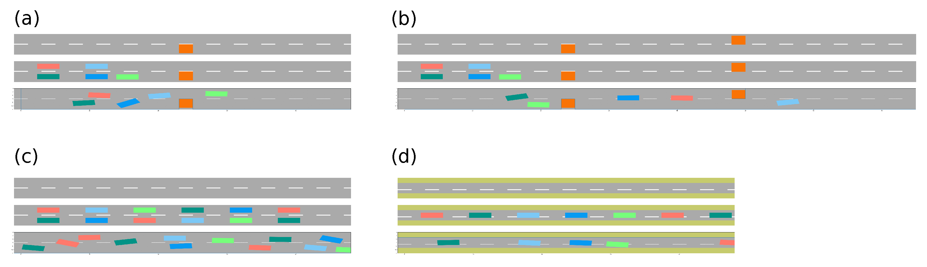
3.3. Scenarios
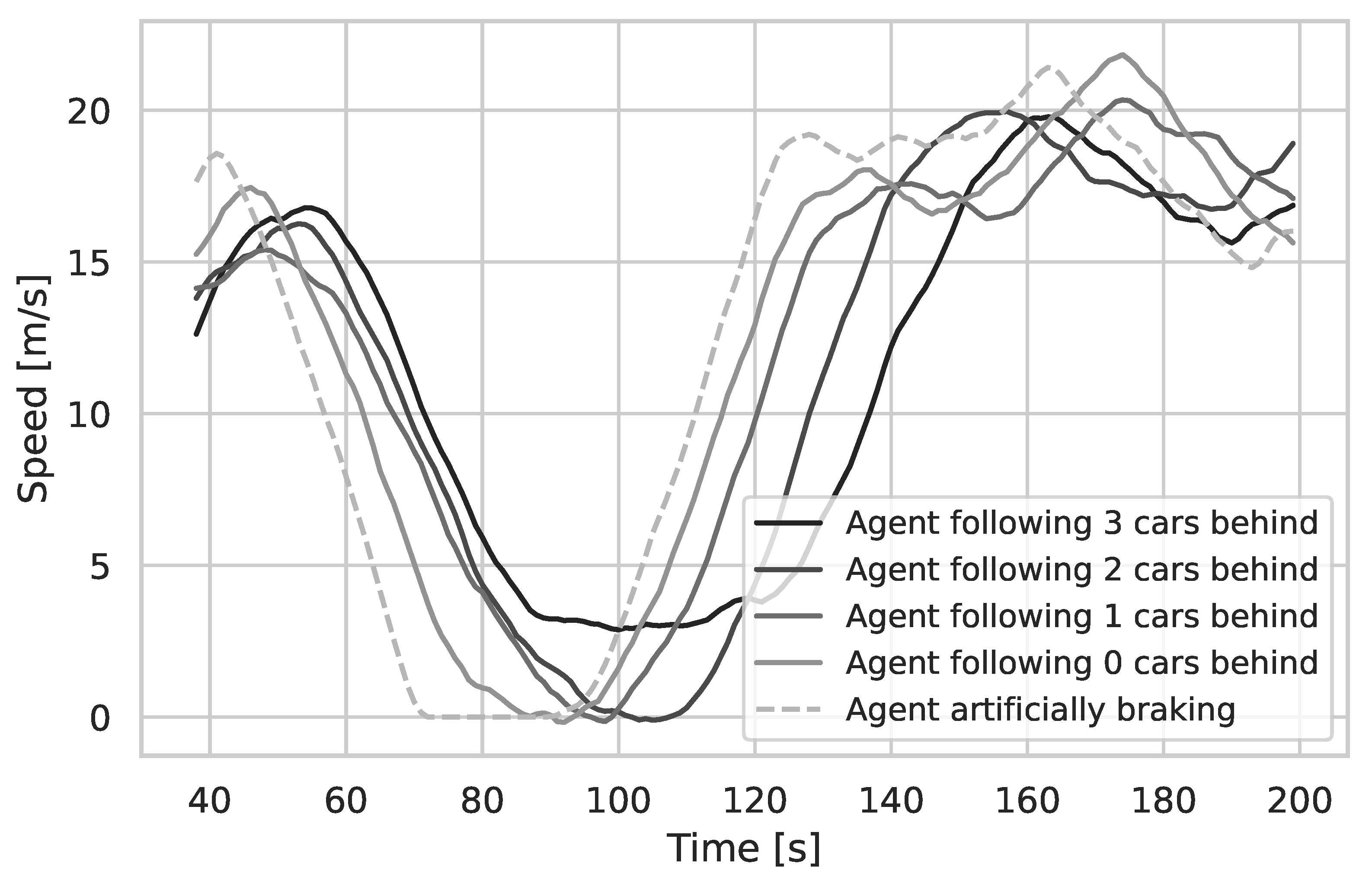
Four different scenarios were developed to assess the performance of the FSX principle: basic; single lane; primary; and secondary. The basic scenario was an open road with a width of 6 m: this width approximately accounted for a two-lane road. The single lane scenario, which was a variant of the basic scenario, was useful to prevent agents from circumventing one another when testing an artificial perturbation of traffic flow. In both the basic and single lane scenarios, the road had no formal end, but looped after 200 m. The primary scenario was built on a similar road, with a single object blocking one lane. The secondary scenario introduced a second obstacle in the opposite lane, at some distance from the first obstacle. In both the primary and secondary scenarios, the road did not loop, but ended. The scenarios are listed in
Table 2, and depicted in
Figure 2.
The starting coordinates were the only distinct feature in the setup of the agents: these coordinates marked the pivot point of the agents, as outlined in
Section 3.2. The initial placement put 3 m between the agents, in their driving direction. The agents all faced towards the same direction, which was also the direction in which their utility function increased. In scenarios with two lanes, the agents were placed in pairs—one in each lane: in this case, the initial lateral distance of their pivot points was 3 m, accounting for
m of actual distance, agent-to-agent. The single agent in scenarios (a) and (b), shown in
Figure 2, was placed
m in front of its follower: this allowed it
m to circumvent the obstacle.
5. Discussion
The discussion of the results is split into two parts: the performance of the developed model itself, followed by the more general topic of utilizing FSX for ABM.
5.1. Model Performance
Using an adaptation of the algorithm developed in [
31], FSX reduced the number of parameters to merely three factors: horizon
; number of walkers
N; and the parameter responsible for balancing exploitation versus exploration,
. With our adaptation, multiple objectives could be separated, allowing for parameterization of single-utility functions using multiple
parameters. While such investigations were beyond the scope of this work, the three parameters assessed in our sensitivity analysis showed significant and distinct influences on the agents’ behavior.
The horizon
and the number of walkers
N work together to increase the density of future state space scanning. While the horizon defines how much an agent anticipates the future, the number of walkers is the actual adjustment of the scanning density [
31]. Our model could not show a significant difference in the influence of horizon versus the number of walkers; however, it seems intuitive that a high number of walkers could not share the effect of a high
in some dynamic environments.
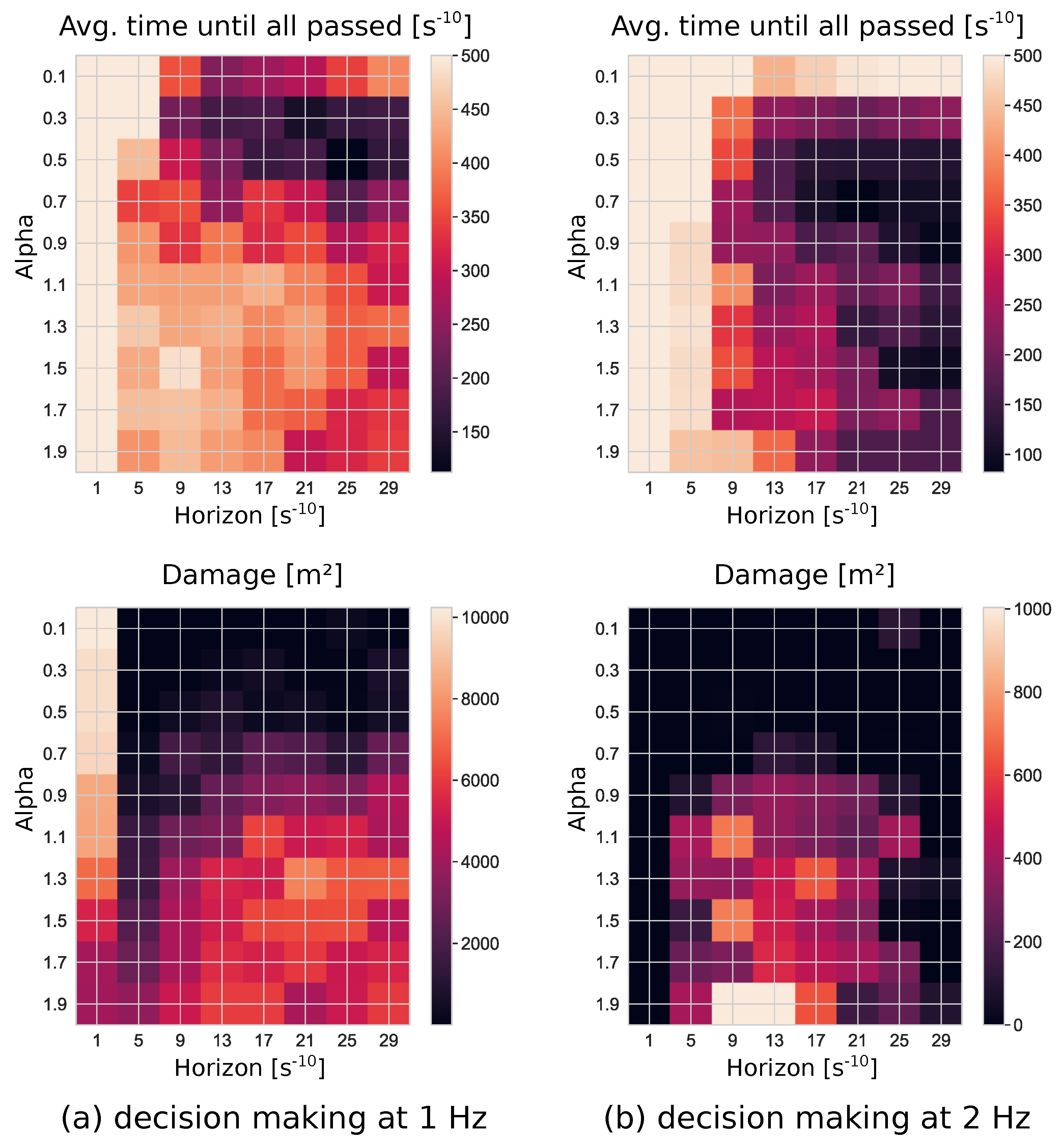
The
parameter showed a significant effect on the performance of the agents. In the case of a high
value, the urgency of the agents to reach their goal on the very right of their map outweighed their struggle to survive: in effect, the agents refused to cooperate, and often consecutively blocked one another. The upper bound of the
parameter in the sensitivity analysis was chosen to be
: this value was in line with the interval given by [
31].
However, while it was paramount to also assess the mistakes made by the agents, the damage measure could be improved. If the agents got locked into an unfavorable position, the damage value could increase vastly, while a fast agent might not collect much overlap with an opponent before it had crossed the area. A more realistic damage measure, including impact velocity, would be necessary for a closer look into the severity of the mistakes made by our agents.
5.2. FSX as a Framework for Agent Intelligence
As the ABM approach progresses, the challenge remains of representing human behavior [
1]. The use of machine learning techniques has thus far been hampered by their demand for large data [
1]. We propose FSX as one “theory of behavior” [
1] by which to model human agents without machine learning. Utilizing FSX, the author of an ABM no longer imposes specific rules of behavior: instead, the agents leverage the ethical imperative of constructivist Heinz von Foerster [
39] as the decision making mechanism. Rules are superseded by the definition of boundaries. Future state spaces external to the model can be introduced via a utility function.
This design principle changes the way that the model author is led to think about the agents’ behavior. The agents utilize their artificial intelligence to their benefit. Instead of imposing what the agents should do, we design their capabilities, i.e., acceleration or deceleration, and boundaries given by the shape of the agent and environment, etc. By shifting the thought process from imposing rules to expressing boundaries, we argue that it becomes more intuitive. In a similar way, defining differential equations comes more naturally than expressing the evolution of state variables directly.
The definition of bounded rationality brought forward by [
15] is based on the two concepts of “search” and “satisficing”: it is possible to interpret FSX in the light of this definition. The search concept is embodied in the walker process. Satisfaction is completed once the horizon is reached, as a result of the walker redistribution process. The density of the search is characterized by the number of walkers. The limit of satisfaction is guarded by the horizon. Thus, a high number of walkers and a high horizon lowers the bound of rationality. This is associated with higher intelligence [
12].
Our analysis of the model patterns suggests that this method, being rule-less, can reproduce the behavior of rule-based models. A traditional, but still widely used [
43] model [
50], and a modern study [
42] serve as a comparison. Future state maximization appears to replicate well the patterns found by [
42,
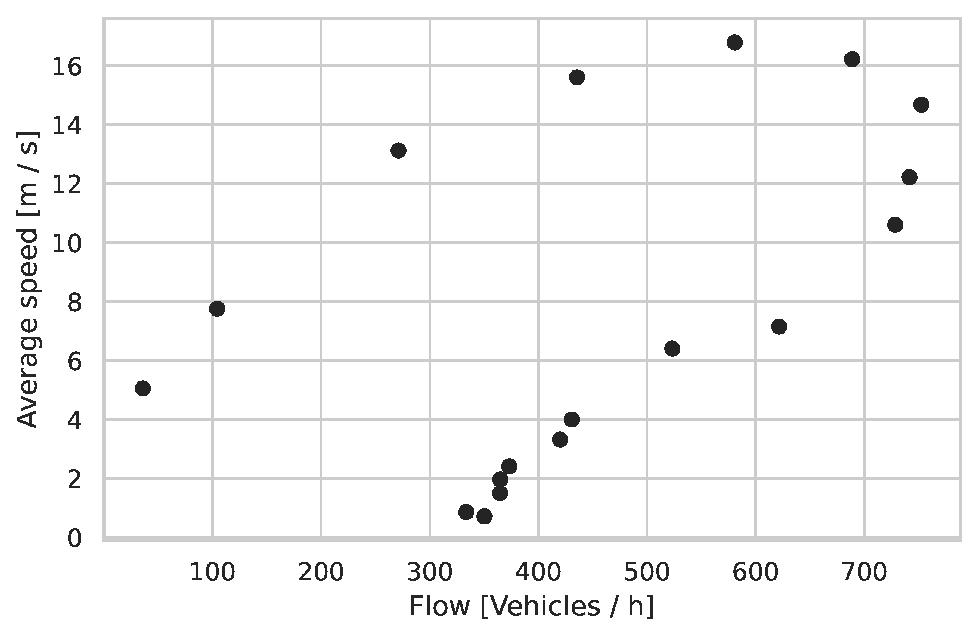
50]: it is, however, not clear if these patterns are not mere emergent phenomena found in any traffic system. No clear connection between the patterns, pointing to specific human behavior, has been found. Nevertheless, the patterns show some key features predominant in human driving: in particular, the disturbance of the traffic flow shows clear signs of a reaction time. This is also implicit in the horseshoe pattern, as it displays a slowdown of the traffic flow in scenarios with a high car density.
As argued by [
51], an actual agent-based traffic simulation distinguishes between the traffic system and its internalized representation used by an agent: this notion agrees with the constructivist interpretation of an agent’s epistemic capabilities. It has been shown that FSX can serve as a computational model of such a notion [
33]. While [
51] modeled a large traffic system, we focused on the microscopical interaction of agents. Internalized information that was crucial to our agents included the estimates of future trajectories. Our model has already succeeded, using a simple extrapolation: however, other heuristics could also be utilized [
32]. More complex models could be exploited to derive trajectories from human behavior [
52].
The low number of the FSX parameters (
,
,
N) in conjunction with the intuitive definition of the degrees of freedom for our agents showed how FSX could be a promising alternative to other artificially intelligent agents, as in [
20], or to rule-based ABMs, as described by [
6]. The damage values showed that the agents were not perfectly rational, but rather acted in certain interests. Moreover, the agents appeared to be interacting independently, as proposed in the definition of an agent by [
4].
A novel finding that we can report is that FSX agents can, in fact, stop cooperating: this could be closely related to the breakdown and respective emergence of structure within the collectivism of the CEF agents, as shown in [
34]. What is novel in our investigations is the introduction of a utility function, as pioneered by [
31].
The separation of objectives, which we conducted within this work, enabled us to independently steer the influence of both survival (exploration) and utility (exploitation): we argue that the
parameter alone, as previously stated by [
31], cannot balance these using a single reward function encoding both survival and utility. Reducing
, in this case, also rendered the agent incapable of striving for survival, as all information about the survival of the walkers was lost. The exploring agent was prone to run into states which were not survivable: this goes against the idea of exploitation versus exploration, which is more aligned with risk-taking versus conservatism.
With our modification, this could no longer happen. For cooperation, a balance between exploration and exploitation had to be struck. Urgency to reach an objective yielded agents too egoistic to make way for a fellow. On the other end of the spectrum, absence of urgency left the agents indifferent enough about the objective to get stuck in sub-optimal situations: it seems that urgency is required to collectively strive for the greater good. This is reminiscent of the finding by [
35], that cooperative behavior can follow from the interaction of egoistic agents.
Another reason why other researchers, such as [
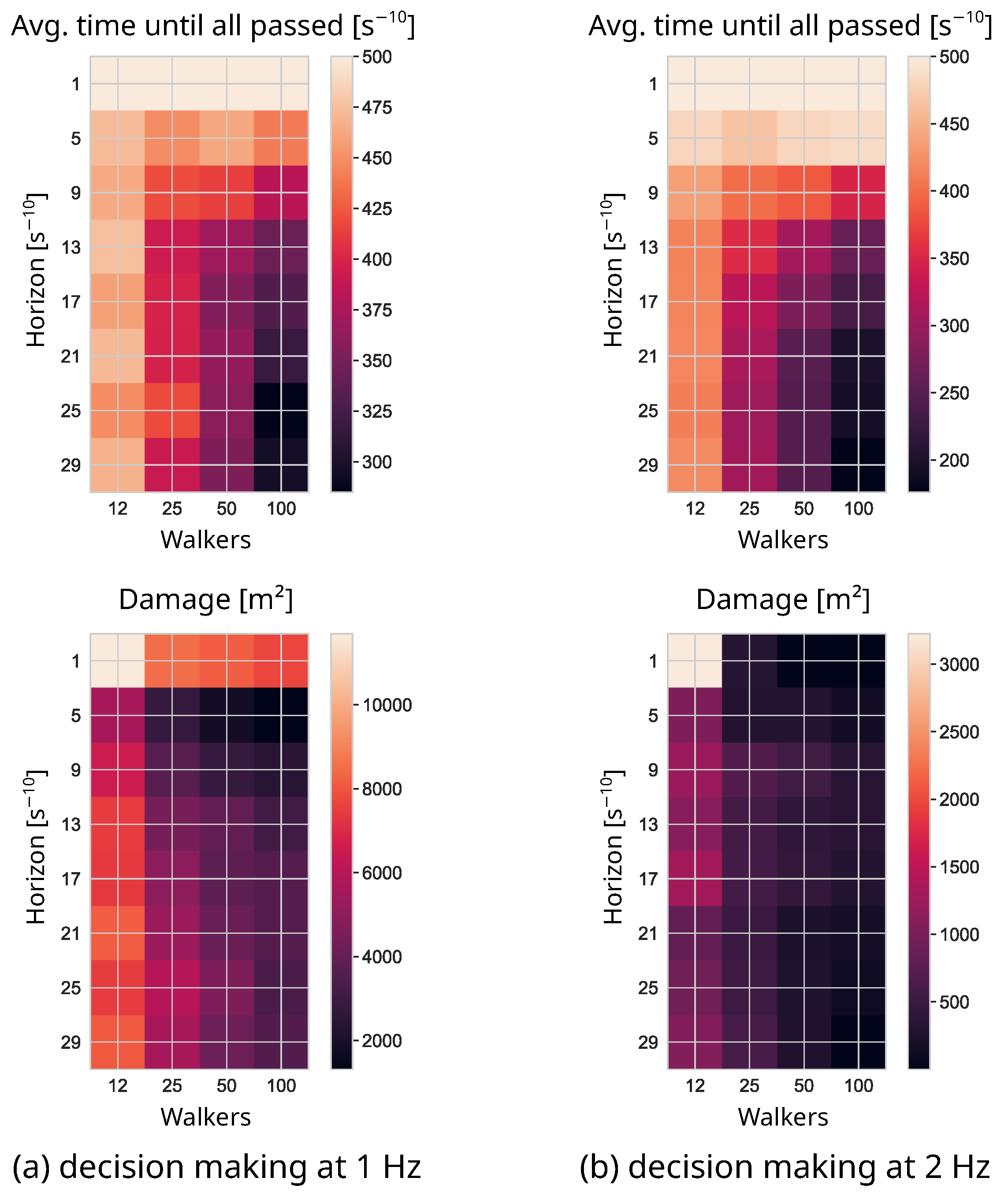
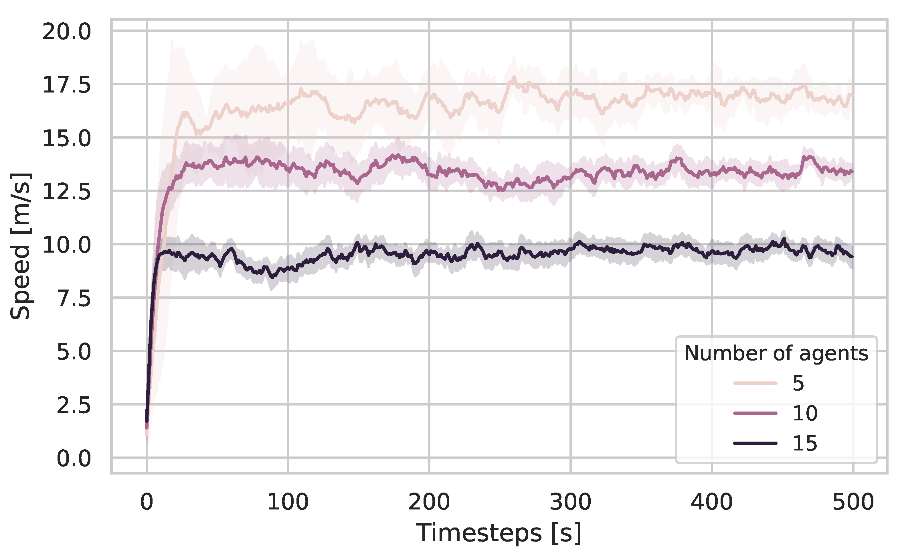
32], discovered the collaboration of their agents could be due to the sequential evaluation of their agents’ decisions and high sample rates. As can be seen in
Figure 3 and
Figure 4, an increased number of decision steps improves the result: it, effectively, reduces the reaction time to the actions of other agents. Due to the sequential calculation, every agent has complete information about its surroundings. If the interval between the time steps is made small enough, the agents can effectively react to everything, and appear to be cooperative. Computationally, however, this is not feasible. A possible alternative would be to ensure a certain scanning density through a “dynamic horizon”. Once the walkers are too dispersed, the scanning is interrupted, and the intermediate result is used.
5.3. Limitations and Further Research
The computational demand of agents utilizing the FSX principle is high: this could render more elaborate investigations time-consuming and expensive. The FSX principle is thus only applicable in cases of systems comprising a few agents. One of the possible options to decrease the demand for computing resources is to reduce the option and/or state space to a low number of discrete points when this is feasible.
However, the research on this novel method is still in its infancy. It is possible that future exploration will decrease the computational demand. The parallel nature of the walker entities offers itself for concurrent computing: one such frontier could be found in a “dynamic horizon” which could reduce the computational demand in certain situations, and improve both computational and intelligent performance. For example, decreasing computational demand would enable robustness and scalability assessment for larger populations of agents, which could be beneficial for studying large networks typical for traffic simulations [
53].
Thus far, only equivalent (homogeneous) agents have been considered. The small number of parameters compared to, for example, an artificial neural network or an accumulation of several rules would make it straightforward to define a heterogeneous population. In addition, the intuitive description of future state expectations also enables creating agents with specific beliefs. One of the future development directions could be the explicit integration of sleepiness, distraction, or aggression into the decision making process of the vehicle driver [
46]: for example, reduced scanning density (considering fewer options) could be employed in case of sleepiness, or a decreased planning horizon, and tolerating more anticipated damage, to model aggression [
54].
Our sensitivity analysis could also establish some foundation for the understanding of the social behavior among future state maximizing agents: however, a microscopic traffic model has only a limited capacity for explaining it. For a more clear insight into the interaction of individual FSX agents, a purpose-made model would be beneficial. Future research could employ simpler models, such as a public-good game, to strengthen the insights into cooperation and its breakdown among such agents.
6. Conclusions
An assessment of the developed agent-based model of small road sections, using FSX agents, shows qualitative similarities to the common car-following model of [
50]. Furthermore, patterns observed in real-world traffic can also be observed when using FSX agents: however, in contrast to the model of [
50], the behavior of these agents is emergent from their thought process, using the FSX principle and the (physical) boundaries applying to them.
Cooperation among FSX agents can, in fact, break down due to limited rationale. The agents can exhibit behavior which could be utilized for models lacking traffic regulations, such as shared spaces. Moreover, scenarios where some agents do not totally abide by the law, are plausible. Hence, FSX could serve as a theoretical foundation for agent-based modeling as an alternative to machine learning algorithms: it could be especially useful in cases with a low abundance of data.
The future state maximization principle shows qualities that render it applicable to ABM. Bounded rationality is implicit in our model: the agents exhibit what could be interpreted as intelligent behavior; moreover, this behavior can be adjusted by varying the horizon and the number of walkers an agent spawns. An additional parameter (
) is available to adjust the influence of a utility function [
31]. We successfully extended the algorithm of [
31], to separate survival from utility dynamics. As the sensitivity analysis shows, these parameters are rather influential: therefore, they can be useful for fitting the model to data.
Models like the one presented can be useful when it comes to training algorithms for autonomous cars in challenging traffic scenarios. Most agent-based models for autonomous vehicles have thus far only considered mesoscopic scenarios of mode and route choice [
41,
55]. Common models cannot depict irrational driving behavior [
42,
45]: FSX agents, like the ones presented in this paper, could fill this gap.
The FSX approach could also be useful for modeling the boundedly rational behavior of human agents in other dynamic situations, such as movement of pedestrians or crowd behavior in emergencies [
56,
57].


