Optimization Model for the Energy Supply Chain Management Problem of Supplier Selection in Emergency Procurement

Abstract

In energy supply chain management (ESCM), the supply chain members try to make long-term contracts for supplying energy stably and reducing the cost. Currently, optimizing ESCM is a complex problem with two social issues: environmental regulations and uncertainties. First, environmental regulations have been tightened in countries around the world, leading to eco-friendly management. As a result, it has become imperative for the energy buyer to consider not only the total operating cost but also carbon emissions. Second, the uncertainties, such as pandemics and wars, have had a serious impact on handling ESCM. Since the COVID-19 pandemic disrupted the supply chain, the supply chain members adopted emergency procurement for sustainable operations. In this study, we developed an optimization model using mixed-integer linear programming to solve ESCM with supplier selection problems in emergency procurement. The model considers a single thermal power plant and multiple fossil fuel suppliers. Because of uncertainties, energy demand may suddenly change or may not be supplied on time. To better manage these uncertainties, we developed a rolling horizon method (RHM), which is a well-known method for solving deterministic problems in mathematical programming models. To test the model and the RHM, we conducted three types of numerical experiments. First, we examined replenishment strategies and schedules under uncertain demands. Second, we conducted a supplier selection experiment within a limited budget and carbon emission regulations. Finally, we conducted a sensitivity analysis of carbon emission limits. The results show that our RHM can handle ESCM under uncertain situations effectively.

1. Introduction

Energy supply chain management (ESCM) pursues long-term contracts for a stable supply of energy. However, some kinds of uncertainties, such as pandemics, natural disasters, and wars, break supply chains and change the demand for energy. In this case, the buyer operates emergency procurement for energy through a short-term contract with suppliers. Even though the short-term contract increases the total cost, the emergency procurement is necessary for sustainable management under uncertainties [1,2]. Therefore, this paper deals with the problem of selecting energy suppliers when uncertain situations occur.

Among the various types of energy supplies, fossil fuels have long been in the spotlight as traditional energy sources that provide essential energy for generating electricity, which is the basis of the industry [3]. Because the calorific value of fossil fuels from each supplier is different, a contract should be made considering the price of fossil fuels, transport distance, and calorific value. The traditional ESCM focuses on selecting a supplier that supplies energy in a timely manner and at a reasonable price [4]. In addition, ESCM attempts to respond to uncertainties to secure supply stability. Sudden events such as pandemics, natural disasters, and financial crises lead to market uncertainty. During the first two years of the COVID-19 pandemic, power consumption in 53 countries decreased by approximately 7.6% each year. During the 2008 global financial crisis, global power consumption fell by approximately 7% each year [5]. Due to these types of uncertainties, it is difficult to predict market conditions and manage energy consumption. Incorrect predictions can cause significant economic costs, such as shortage and inventory costs [1,6]. Therefore, many governments that cannot produce fossil fuels are interested in ESCM replenishing fossil fuels from suppliers around the world [7].

In addition, as carbon emission regulations have been strengthened in recent years, carbon emissions should also be considered in ESCM [8]. It is well known that fossil fuels emit carbon during production. When fossil fuels are transported by ships, a large amount of carbon is emitted. Thus, the current ESCM should consider carbon emissions during the production and transportation of fossil fuels by suppliers.

To solve the above issues, many ESCM studies focus on the long-term contract model based on game theory and mathematical programming. However, those models cannot handle uncertainties. Only a few studies dealt with the stochastic models for handling uncertainty problems [1,9]. This paper developed an optimization model using mixed integer linear programming (MILP) to solve the ESCM problem of supplier selection in emergency procurement under uncertainties and carbon emission regulations. Even though the advantage of MILP is that it can guarantee finding the optimal solution compared to other methods, the weakness of MILP is the deterministic characteristics that cannot handle uncertainty. Thus, the rolling horizon method (RHM) is applied to cope with uncertain situations. This method is used to solve mathematical programming models by dividing the planning horizon into smaller sub-horizons and repeatedly updating new information [10]. Due to this, RHM can solve emergency procurement situations.

This study has two main contributions. First, we formulated an optimization model based on MILP for ESCM with carbon emissions. The model considers non-zero lead times, uncertain demands, and limited resources such as ships and port capacity. The caloric value is considered because the efficiency of the supplier’s fuel is different. Second, RHM was developed as a solution methodology for handling uncertain demands. The thermal power plant can update demand information and determine replenishment strategies during the planning horizon.

The remainder of this paper is organized as follows: Section 2 presents the literature review. The assumptions and problem definitions are presented in Section 3. The mathematical model is described in Section 4. Numerical experiments are presented in Section 5. Both academic and managerial insights are presented in Section 6. Finally, the conclusions are presented in Section 7.

2. Literature Review

This study focused on three research areas: a basic study of ESCM with supplier selection, SCM with emergency procurement, and carbon emissions in ESCM.

Most basic studies on ESCM consider markets, including demand forecasting and contracts. An et al. [11] focused on a lignocellulosic biomass and biofuel supply chain that considers multiple commodity flows, ranging from biomass suppliers to biofuel customers. This model deals with a production and distribution system that determines facility locations, capacities, technology, and material flows to maximize profits. Manenti and Rovaglio [12] presented an optimization model for industrial gas supply chains under binding contracts that place tight limits on suppliers. Akgul et al. [13] developed a multi-objective programming model for biofuel supply chains considering economic and environmental objectives. Balaman and Selim [14] presented a multi-objective mixed-integer programming (MOMIP) model, which proposed both the design and management of sustainability and cost effectivity under both seasonally variable resources and fluctuations of the system parameters. Only a few researchers have considered supplier selection in ESCM. You et al. [15] developed a multi-objective MIP model to optimize both the design and planning of cellulosic ethanol supply chains under economic, environmental, and social objectives. Some researchers have integrated economic objectives and carbon emissions in various ways, such as the total annual cost, life cycle greenhouse gas emissions, and accrued local jobs. Osmani and Zhang [16] proposed a two-stage stochastic MIP model to maximize the expected profit while minimizing the environmental impact of a lignocellulosic bioethanol supply chain under biomass supply, bioethanol demand, and biomass/bioethanol price uncertainties. Jauhari et al. [7] proposed an inventory model for an electricity-supply chain. Most studies suggest a mathematical model for designing or planning SCM based on long-term contracts, so it is difficult to apply it in uncertain situations.

After COVID-19, some researchers focus on emergency procurement for SCM. One of the key challenges in selecting suppliers determines which suppliers to contact and how to distribute orders among them. In emergency procurement, it is important to carefully select suppliers and allocate orders. Harland et al. [17] considered the healthcare product with emergency procurement and supply management maturity during COVID-19. They focused on the early stage of COVID-19 from 23 countries and suggested the awareness-motivation-capability (A-M-C) framework in the healthcare SCM. Scala and Lindsay [18] interviewed the public sector supply chain actors in healthcare during the pandemic disruption. They discovered that the relationships with suppliers pre-pandemic did not increase the visibility of tiers within the supply chain. Lin et al. [19] suggested that the newsvendor model solve emergency procurement during the COVID-19 pandemic. Only a few studies suggest that the mathematical model solve emergency procurement in the pandemic. It was difficult to find studies related to emergency procedures in ESCM.

Due to growing concerns and an interest in environmental issues in recent years, many studies have begun to consider carbon emissions in ESCM. Mishra et al. [20] developed a sustainable electricity supply chain mathematical model that assumes linear price-dependent customer demand, where the price is a decision variable among setup costs and carbon emissions. Niesseron et al. [21] developed a mathematical model that can be extended to an entire supply chain network to address sustainability within the network by comparing the environmental impact to cost optimization. Iqbal et al. [22] presented an energy supply chain model to satisfy the dual objectives of zero waste and minimum energy consumption to protect the environment and conserve energy resources. As most ESCM studies consider carbon emission, this study also intends to consider carbon emission.

Based on the literature review, we focused on ESCM for buyers to select suppliers who provide energy sources which include coal, oil, and gas. Through this, the buyer chooses suppliers and orders energy while minimizing economic costs and carbon emissions under uncertainties.

Table 1. Comparison of the contributions of different studies.

Author	Contract	Energy	Period	Method
An et al. [11]	Long-term	Biofuel	Multi	MIP
Osmani and Zhang [16]	Long-term	Bio ethanol	Multi	Stochastic
Mishra et al. [20]	Long-term	Electricity	Single	NLP
Jauhari et al. [7]	Long-term	Fossil fuel	Single	NLP
Niesseron et al. [21]	Long-term	Formal energy	Single	NLP
Iqbal et al. [22]	Long-term	Formal energy	Single	NLP
Present paper	Short-term	Fossil fuel	Multi	MILP

MIP: mixed-integer programming; NLP: Nonlinear programming.

shows the comparison of the contributions of different studies.

3. Assumptions and Problem Definition

A full list of all notations is presented in Appendix A. The following assumptions were made for this system:

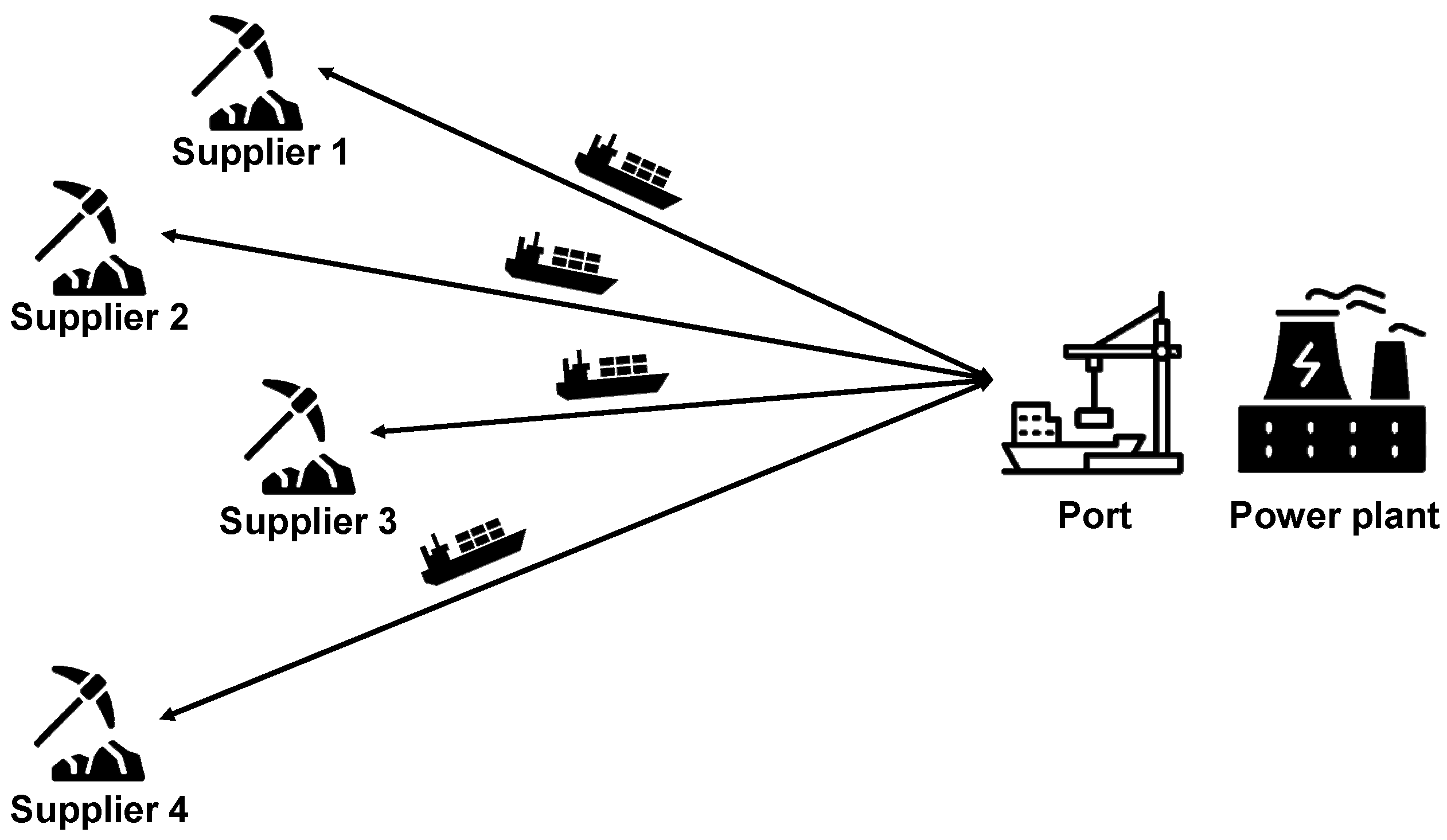
• The system consists of a single thermal power plant and multiple suppliers with one type of fossil fuel such as coal, fuel, and natural gas. In terms of ESCM, the thermal power plant attempts to select suppliers that minimize both the total cost and carbon emissions.
• Each supplier produces different qualities of fossil fuel; therefore, there are different calorific values for the fossil fuel produced.
• To handle the calorific value level, the thermal power plant applies an order-up-to level policy.
• The thermal power plant transports fossil fuels via ships. In addition, the thermal power plant has various classes of ships, which are limited in number.
• The transportation time is the round-trip time, and the system considers a non-zero lead time.
• Based on the caloric value demand, the thermal power plant orders the fossil fuel from each supplier at the beginning of the period. Then, the ordered fuel is replenished after the lead time from each supplier.
• Regarding the lead time, the preordered fuel should arrive at the beginning of the planning horizon.
• The thermal power plant has a safety stock in terms of its calorific value to provide good service.
• The thermal power plant has a limited budget.
• The thermal power plant has a limited port capacity, and only a certain number of ships can come to the port at the same time.

Problem Definition

This system considers ESCM of supplier selection in emergency procurement under the uncertain situations, such as pandemics or wars. In emergency procurement, the buyer makes a short-term contract with the supplier according to market demand changes. This ESCM system consists of a thermal power plant and multiple suppliers that produce one type of fossil fuel such as coal, natural gas, or oil. Fossil fuels have different qualities because of the suppliers’ locations and production systems, and, therefore, the energy from each supplier has different calorific values. A thermal power plant uses various types of ships to transport fossil fuels. In addition, the thermal power plant, a buyer, has limited port capacity, limited budget, and carbon emission limitations. In terms of environmental sustainability, the thermal power plant considers carbon emissions during production and transportation from suppliers. Based on the above conditions, the thermal power plant must consider both the economic and environmental impact when ordering fossil fuels. In short, the thermal power plant attempts to select suppliers who supply high-quality fossil fuels with low carbon emissions. Figure 1 illustrates the study environment.

4. Mathematical Model

This chapter presents a MILP model to minimize the total cost of energy supply chains consisting of a single thermal power plant and multiple suppliers. A thermal power plant orders fossil fuels from one or more suppliers based on the demand for energy and the number of ships. The thermal power plant also considers the carbon emissions resulting from production and transportation from the supplier. In terms of optimizing ESCM, the thermal power plant makes decisions to minimize the total cost while considering carbon emission limits and resources. The objective function, which measures the total cost of operating the ESCM, consists of the ordering, transportation, and holding costs. The ordering cost is incurred when fossil fuel is ordered from supplier $i$ in period $t$. Thus, the ordering cost of supplier $i$ in period $t$ is calculated as follows:

$${\displaystyle \sum }_{i=1}^I{\displaystyle \sum }_{t=1}^T{A}_i{\alpha }_{it}$$

(1)

After ordering, the thermal power plant transports fossil fuels using ships from supplier $i$ in period $t$. Transportation cost is related to the distance between supplier $i$ and ship class $j$.

$${\displaystyle \sum }_{i=1}^I{\displaystyle \sum }_{j=1}^J{\displaystyle \sum }_{t=1}^T{R}_{ij}{Y}_{ijt}$$

(2)

The expected calorific value capacity of a thermal power plant for period $t$ was approximated as the average of the start and end periods of the on-hand calorific value capacity. Thus, the holding cost of the calorific value capacity of the thermal power plant for period $t$ is denoted as follows:

$${\displaystyle \sum }_{t=1}^T\frac{h_t\left(S_t+l_t\right)}{2}$$

(3)

Using the above-calculated costs, the objective function(Z) is computed as shown below.

$$Z={\displaystyle \sum }_{i=1}^I{\displaystyle \sum }_{t=1}^T{A}_i{\alpha }_{it}+{\displaystyle \sum }_{i=1}^I{\displaystyle \sum }_{j=1}^J{\displaystyle \sum }_{t=1}^T{R}_{ij}{Y}_{ijt}+{\displaystyle \sum }_{t=1}^T\frac{h_t\left(S_t+l_t\right)}{2}+{\displaystyle \sum }_{i=1}^I{\displaystyle \sum }_{t=1}^{T}p{x}_{it}{X}_{it}$$

(4)

Then, the following MILP model $Z$ can be developed.

$$Min Z$$

(5)

$$\mathrm{subject}\mathrm{to}$$

$$S_t-d_t=l_t t=1, 2,\cdots ,T$$

(6)

$$l_{t-1}+{\sum }_{i=1|t-L_i\le 0}^I{\gamma }_{it}{\tilde{X}}_{it-L_i}+{\sum }_{i=1|t-L_i>0}^I{\gamma }_{it}{X}_{it-L_i}=S_t t=1, 2,\cdots ,T$$

(7)

$$X_{it}\le P_{it} i=1, 2,\cdots ,I, t=1, 2,\cdots ,T$$

(8)

$$X_{it}\le {\sum }_{j=1}^J{C}_j{Y}_{ijt} i=1, 2,\cdots ,I, t=1, 2,\cdots ,T$$

(9)

$$b\le l_t t=1, 2,\cdots ,T$$

(10)

$${\sum }_{i=1}^{I}CO{P}_i{X}_{it}+{\sum }_{i=1}^I{\sum }_{j=1}^{J}CO{T}_{j}DI{S}_i{Y}_{ijt}\le C{E}_t t=1, 2,\cdots ,T$$

(11)

$${\sum }_{i=1}^I{\sum }_{j=1}^J{Y}_{ijt}\le N t=1,2,\cdots ,T$$

(12)

$${\sum }_{i=1}^I{Y}_{ijt}\le U_{jt} j=1, 2,\cdots ,J, t=1, 2,\cdots ,T$$

(13)

$$X_{it}\le M{\alpha }_{it} i=1, 2,\cdots ,I, t=1, 2,\cdots ,T$$

(14)

$${\sum }_{i=1}^{I}p{c}_i{X}_{it}\le B t=1, 2,\cdots ,T$$

(15)

$$X_{it}\ge 0, real variable i=1, 2,\cdots ,I, t=1,2,\cdots ,T$$

(16)

$$S_t, l_t\ge 0, real variable t=1, 2,\cdots ,T$$

(17)

$$Y_{ijt}\ge 0, integer variable i=1, 2,\cdots ,I, t=1, 2,\cdots ,T,j=1, 2,\dots ,J$$

(18)

$${\alpha }_{it}, binary variablei=1, 2,\cdots ,I, t=1, 2,\cdots ,T$$

(19)

Equation (5) shows the MILP problem to minimize Z. Equation (6) shows the relationship between calorific value capacity and energy demand. The calorific value capacity at the end of period $t$ is the replenishment level at the start of period $t$ subtracted from the demand for calorific value in period $t$. In Equation (7), the first term denotes the initial calorific value at period $t$. The second part presents the calorific value of the pre-order quantity that the thermal power plant orders from each supplier before starting the planning horizon. The third part denotes the calorific value of the order quantity of each supplier after the start of the planning horizon. Finally, the replenishment level is satisfied by the sum of the three parts. In Equation (8), the order quantities from supplier $i$ cannot exceed the supply of supplier $i$. Equation (9) ensures that the order quantities from supplier $i$ do not exceed the capacity of the ships. According to Equation (10), the calorific value capacity must exceed the safety stock at all times. Equation (11) states that carbon emissions during production and transportation cannot be greater than the thermal power plant’s maximum limit of carbon emissions because of carbon emission regulations. Equation (12) indicates that the number of ships cannot exceed the port capacity of a thermal power plant. Equation (13) ensures that the thermal power plant has a limited number of ship classes $j$. Equation (14) controls the ordering cost when an order is issued. Equation (15) shows the budget limitation of the thermal power plant.

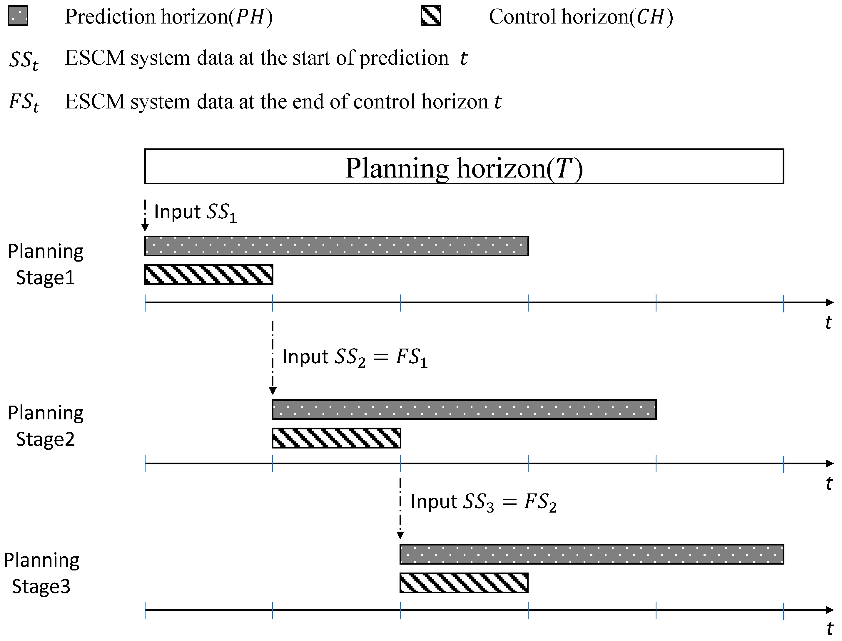
5. Rolling Horizon Method

To handle the uncertainty of energy consumption, the information on market conditions has to be updated iteratively. The RHM solves mathematical programming models by dividing the entire time into smaller scheduling sub-horizons and repeatedly updating new information. The method is more efficient at planning and scheduling problems because it reduces the calculation time and, at the same time, updates information each period time rather than solving for the entire horizon. Yu and Yang [23] used the RHM to solve the crane scheduling problem of MILP in a hybrid storage container terminal. Li and Ierapetritou [24] proposed an RHM to address the integrated production planning and scheduling optimization problem. Silvente et al. [25] used an RHM that periodically updates input data information to solve MILP problems in ESCM for demand planning in microgrids. Even though the RHM does not guarantee an optimal solution, many researchers addressed the RHM for handling uncertainties.

The time flow of the RHM is divided into the planning horizon and two detailed horizons: the prediction horizon and the control horizon. The prediction period enhances schedule management by forecasting demand for future periods at the beginning of the control horizon. Figure 2 shows the concept of RHM.

RHM

Step 1. Set input parameter

Step 1.1.

Input the planning horizon $T$, the control horizon $CT$ and the prediction horizon $PT$

Step 1.2.

$PS$, set the planning stage as 1

Step 2. Solve MILP

Step 2.1.

$S{S}_{PS}\leftarrow$ Measure the ESCM system at the start of period $t$

Step 2.2.

Input the data of $S{S}_{PS}$

Step 2.3.

Calculate the optimal solution

Step 3. Set

Step 3.1.

$F{S}_{PS}\leftarrow$ Record the difference between the initial replenishment level of inventory and actual demand at the end of the control time horizon.

Step 4. Check iteration condition

Step 4.1.

If $PS$ < $T$, move to Step 4.2. Otherwise, calculate the total cost and move to Step 5

Step 4.2.

Calculate the total cost, set $S{S}_{PS+1}=F{S}_{PS}$ and move to Step 2 by applying $PS\leftarrow PS+1$.

Step 5. End RHM and organize the recorded historical costs at each $PS$

6. Numerical Experiment

In this section, we describe three types of numerical experiments conducted to verify the performance of the proposed MILP model and RHM. In the first experiment, we tested the effectiveness of the RHM compared with a deterministic method (DM) under various demand patterns. In the second experiment, a sensitivity analysis of the maximum limit of carbon emissions was performed. The proposed MILP and RHM models were coded using Python 3.6.0. The three experiments were performed using CPELEX 12.0.0 on a computer with an Intel i7-3770 CPU at 3.4 GHz and 16 GB RAM.

For both experiments, we focused on the case of a coal supply chain with five suppliers and considered one type of demand pattern, such as seasonal demand. We set $M$ to a large value (1,000,000). The percent deviation, $100*(T{C}_{RHM}-T{C}_{DM})/T{C}_{DM}$, is used for measuring efficiency. The randomly selected data are shown in

Table 2. The input parameters for each supplier.

$\mathbf{Supplier}\left(i\right)$		1	2	3	4	5
$A_i$		75	78	93	70	105
$P_{it}$		100	100	500	500	100
${\gamma }_{it}$		0.3	0.2	0.6	0.5	0.6
$CO{P}_i$		27	33	35	38	48
$DI{S}_i$		10,000	4000	17,000	12,000	19,000
$L_i$		1	1	1	1	1
$\mathrm{Ship}\mathrm{class}\left(j\right)$
$R_{ij}$	1	3726	8326	8061	4577	8326
	2	3244	7429	6681	4250	7429

,

Table 3. The input parameters for the thermal power plant.

${\mathit{l}}_1$	${\mathit{h}}_{\mathit{t}}$	$\mathit{b}$	$\mathit{N}$	$\mathit{C}{\mathit{E}}_{\mathit{t}}$
100	21	100	8	200,000

and

Table 4. The input parameters for the ship classes.

Ship Class	${\mathit{C}}_{\mathit{j}}$	${\mathit{U}}_{\mathit{j}\mathit{t}}$	$\mathit{C}\mathit{O}{\mathit{T}}_{\mathit{j}}$
1	60	10	2.8
2	40	8	3.1

. Table 2 and Table 3 list the input parameters for each supplier and a thermal power plant, respectively. Table 4 presents the data on the ship classes.

6.1. Effectiveness Test of the RHM

The purpose of this experiment was to test the effectiveness of the RHM by comparing its results with those of the DM under various demand patterns. As explained in the previous section, the RHM iteratively updates the information on the energy demand and inventory level in a MILP model so that it can handle uncertain information. In contrast, the DM is a traditional approach that solves the MILP model once at the beginning of the planning horizon, and the obtained result of the DM is used throughout the entire horizon. The time horizon is 12 months, and the rolling period was set to values of 2–12 months.

Table 5. The results of the comparative experiment.

Rolling Period	$\mathbf{Total}\mathbf{Cost}\mathbf{of}\mathbf{RHM}\left(\mathit{T}{\mathit{C}}_{\mathit{R}\mathit{H}\mathit{M}}\right)$		$\mathbf{Total}\mathbf{Cost}\mathbf{of}\mathbf{DM}\left(\mathit{T}{\mathit{C}}_{\mathit{D}\mathit{M}}\right)$
		Percent Deviation
2	149,772.07	1.66	147,327.07
3	148,609.07	0.87
4	144,662.07	−1.81
5	146,605.06	−0.49
6	143,917.06	−2.31
7	144,746.07	−1.75
8	141,093.06	−4.23
9	141,681.06	−3.83
10	142,642.06	−3.18
11	148,959.06	1.11
12	147,327.07	0.00

presents the results of the comparative experiment.

As shown in Table 5, most RHM has lower costs than DM. Rolling period 8 resulted in an optimal solution, which obtains a percent deviation of −4.23. However, it is noted that several cases of RHM, rolling periods 2, 3, and 11, obtain lower efficiency than the DM. If the decision maker cannot set the optimal rolling period for updating market information, the efficiency of RHM is less than DM. Although the value obtained in rolling period 8 is the optimal value in the current problem situation, it may not be the best in other experimental situations [25].

6.2. Experiment of Supplier Selection According to Budget

To handle the realistic problem, we check which suppliers are selected according to the buyer’s budget. In general, when a supplier produces energy, there is a trade-off between carbon emissions and costs. If a supplier invests a lot of money in facility investments to reduce carbon emissions, energy sales costs increase to recover the investment. Therefore, in this experiment, when the buyer’s total budget is limited, we examine which supplier is selected considering the trade-off between carbon emissions and sales costs. The lead time of the supplier is 1. The time horizon is 4 months, and the rolling period is fixed 3. Additionally, we set that suppliers with low sales prices have low energy efficiency. The input parameters of each supplier were assumed by random numbers from the probability distributions noted in

Table 6. Input data for second experiment.

${\mathit{A}}_{\mathit{i}}$	${\mathit{P}}_{\mathit{i}\mathit{t}}$	$\mathit{C}\mathit{O}{\mathit{P}}_{\mathit{i}}$	${\mathit{R}}_{\mathit{i}\mathit{j}}$	${\mathit{d}}_{\mathit{t}}$	$\mathit{R}\mathit{e}\mathit{a}\mathit{l} {\mathit{d}}_{\mathit{t}}$
$\left[5, 15\right]$	$\left[100, 300\right]$	$\left[2, 5\right]$	$\left[0.2, 0.6\right]$	$\left[270\right]$	$\left[250, 290\right]$

. The randomly selected data for suppliers are shown in

Table 7. Supplier’s carbon emissions during production and purchase costs.

$\mathbf{Supplier}\left(\mathit{i}\right)$	1	2	3	4	5
${\gamma }_{it}$	0.75	0.6	0.7	0.4	0.55
$p{c}_i$	14	11	12	9	10
$DI{S}_i$	12,528	12,358	13,467	6078	9101

.

Table 8. Output of the comparison experiment.

Budget Limit ($)	Iteration	Supplier Selection					Total Cost of RHM ($)
		1	2	3	4	5
4400	-	-	-	-	-	-	Infeasible
4600	1	$\surd$	-	-	-	-	53,412.6
	2	$\surd$	$\surd$	$\surd$	-	$\surd$
	3	$\surd$	$\surd$	$\surd$	$\surd$	-
	4	-	-	-	-	-
4800	1	$\surd$	-	-	-	-	52,480.5
	2	$\surd$	$\surd$	$\surd$	$\surd$	-
	3	$\surd$	$\surd$	$\surd$	$\surd$	-
	4	-	-	-	-	-
5000	1	$\surd$	-	-	-	-	50,800.7
	2	$\surd$	-	$\surd$	$\surd$	-
	3	$\surd$	$\surd$	$\surd$	$\surd$	-
	4	-	-	-	-	-
5200	1	$\surd$	-	-	-	-	50,800.7
	2	$\surd$	-	$\surd$	$\surd$	-
	3	$\surd$	$\surd$	$\surd$	$\surd$	-
	4	-	-	-	-	-

shows which suppliers are selected during four iterations, according to a limited budget. In all cases, no order is placed in the fourth iteration, because the lead time is non-zero. A buyer with less budget selects an energy-efficient supplier even if the transportation cost increases due to the distance. On the other hand, a buyer with large budget orders energy from a supplier who has low-energy efficiency and is located close to the buyer. It was confirmed that there is a difference in the total cost minimization and purchase efficiency depending on the buyer’s available budget.

6.3. Effect of the Maximum Limit of Carbon Emissions

In this experiment, we evaluated how the total cost of RHM would change depending on the maximum limit of carbon emissions during production and transportation from the supplier. The maximum limit of carbon emissions varied from 200,000 to 225,000. Based on the results of the first experiment, the rolling period 8 was also used in this section as it resulted in the lowest cost.

Table 9. The results of the sensitivity analysis of the maximum limit of carbon emissions.

$\mathbf{Maximum}\mathbf{Limit}\mathbf{of}\mathbf{Carbon}\mathbf{Emissions}\left(\mathit{C}{\mathit{E}}_{\mathit{t}}\right)$	Total Cost ($)
125,000	212,533.08
150,000	161,070.07
175,000	154,999.06
200,000	141,093.06
225,000	141,093.06

shows how the total cost changed as the maximum limit of carbon emissions varied. When the maximum limit of carbon emissions was lowered to 175,000, the total cost appeared to be higher than the previous cost. However, from the time when the limit was increased to 200,000, the total cost was fixed. Even if regulations on carbon emissions are tightened, the minimum cost can be maintained under constraints. This result reveals the trade-off between carbon emissions and economic cost. If more money is spent, a thermal power plant can reduce carbon emissions and vice versa.

7. Academic and Managerial Insights

7.1. Academic Insights

This paper presents a basic study on emergency procedures arising from uncertainties (pandemic, natural disaster, war, etc.) in the ESCM field, which has not been studied much before. In the event of a pandemic or other situation, the existing SCM collapses, so buyers make short-term contracts based on market demand and supplier’s situation every period. Due to this, this study develops a MILP model that considers ESCM of supplier selection in emergency procurement. In addition, RHM, an algorithm that updates demand and supplier situations every period, was applied. The RHM is a well-known method used to solve deterministic problems of mathematical programming models. This study is the first to consider supplier selection and replenishment planning for ESCM in emergency procurement.

7.2. Managerial Insights

For decision-makers, uncertainty causes the existing SCM to collapse, so our finding suggests a short-term contract with a new supplier until the market stabilizes. The RHM can be used to determine the appropriate periods to apply in short-term decisions for thermal power plants. The decision-makers can adjust the prediction horizon according to their judgment to determine planning. Under emergency procurement, a thermal power plant can enter into a contract with a supplier based on either the carbon emissions during production and transportation or the quality of fossil fuel. If the carbon emission exceeds a specific amount, it does not affect the total cost of ESCM. In this case, the thermal power plant could sell carbon emission rights to other thermal power plants through the carbon cap-and-trade program. Consequently, this study makes it possible to realize eco-friendly management in terms of carbon emissions.

8. Conclusions and Suggestions for Future Research

Recently, COVID-19 has caused the collapse of SCM based on long-term contracts, and many supply chain members have conducted emergency procurement through short-term contracts in response to demand. Short-term contracts are more expensive than long-term contracts, but they are essential in situations where SCM has collapsed or demand increases. In addition, buyers can have different suppliers for each contract depending on the market and supplier situation [2]. Thus, the objective of this paper is to focus on an optimization model for ESCM of supplier selection in emergency procurement.

The proposed MILP model in which a thermal power plant (buyer) selects a fossil fuel supplier considering carbon emissions and the thermal power plant’s limited resources. Each supplier produces different qualities of fossil fuels based on its location and production system. This study considered two types of carbon emissions: production and transportation. Fossil fuels can be transported by various types of ships. A thermal power plant can have limited port capacity and carbon emissions. In addition, the system considers market uncertainties. To solve the MILP model under uncertain situations, such as a pandemic, natural disaster, and wars, the RHM was developed.

To check the performance of the proposed MILP model and RHM, we conducted (1) a comparative experiment using RHM and DM, (2) supplier selection under a limited budget, and (3) an effect of the maximum limit of carbon emissions. In the comparative experiment, RHM with rolling period 8 dominates DM. The second experiment confirmed that there is an optimal budget under limited carbon emissions. It was found that if there was more than a certain budget, the total cost could no longer be minimized. The third experiment’s results showed that the RHM did not increase when the maximum limit of carbon emissions was between 200,000 and 225,000. Therefore, the RHM resulted in lower costs than the DM, and we showed that even if regulations on carbon emissions become more stringent, the minimum cost of the RHM can be maintained under constraints.

The limitations of this study and considerations for follow-up studies are as follows: first, we did not consider the trade-off relationship between transportation costs and carbon emission costs. Further analyses should be conducted in follow-up studies to consider this relationship. Second, we considered the transportation of fuel only via sea and not ground. A follow-up study is needed to develop a model that considers the supply of fuel via land and rail. Third, this study considered only carbon emissions from a single energy source. Follow-up studies should consider multiple energy sources. Fourth, additional business restrictions and costs, such as unloading and demurrage, should be identified and reflected in the repair model. This research model is expected to provide management decision support regarding the supply and demand of raw energy materials in the actual power industry through scientific management methods.

References

1. Lee, J.H. Energy supply planning and supply chain optimization under uncertainty. J. Process Control 2014, 24, 323–331. [Google Scholar] [CrossRef]
2. Huang, H.; Li, X.; Liu, S. Loss Aversion Order Strategy in Emergency Procurement during the COVID-19 Pandemic. Sustainability 2022, 14, 9119. [Google Scholar] [CrossRef]
3. Machol, B.; Rizk, S. Economic value of US fossil fuel electricity health impacts. Environ. Int. 2013, 52, 75–80. [Google Scholar] [CrossRef] [PubMed]
4. Li, J.; Wang, L.; Tan, X. Sustainable design and optimization of coal supply chain network under different carbon emission policies. J. Clean. Prod. 2020, 250, 119548. [Google Scholar] [CrossRef]
5. IEA. Global Energy Demand to Plunge This Year as a Result of the Biggest Shock Since the Second World War; IEA: Paris, France, 2020; Available online: https://www.iea.org/news/global-energy-demand-to-plunge-this-year-as-a-result-of-the-biggest-shock-since-the-second-world-war (accessed on 15 January 2022).
6. Emenike, S.N.; Falcone, G. A review on energy supply chain resilience through optimization. Renew. Sustain. Energy Rev. 2020, 134, 110088. [Google Scholar] [CrossRef]
7. Jauhari, W.A.; Melinda, I.D.; Rosyidi, C.N. Inventory-based optimization of a two-echelon fossil-fuelled energy storage system. Int. Trans. Electr. Energy Syst. 2020, 30, e12256. [Google Scholar] [CrossRef]
8. Rogelj, J.; Den Elzen, M.; Höhne, N.; Fransen, T.; Fekete, H.; Winkler, H.; Schaeffer, R.; Sha, F.; Riahi, K.; Meinshausen, M. Paris Agreement climate proposals need a boost to keep warming well below 2 C. Nature 2016, 534, 631–639. [Google Scholar] [CrossRef] [PubMed] [Green Version]
9. Naini, S.G.J.; Aliahmadi, A.R.; Jafari-Eskandari, M. Designing a mixed performance measurement system for environmental supply chain management using evolutionary game theory and balanced scorecard: A case study of an auto industry supply chain. Resour. Conserv. Recycl. 2011, 55, 593–603. [Google Scholar] [CrossRef]
10. Fattahi, M.; Govindan, K. Data-driven rolling horizon approach for dynamic design of supply chain distribution networks under disruption and demand uncertainty. Decis. Sci. 2022, 53, 150–180. [Google Scholar] [CrossRef]
11. An, H.; Wilhelm, W.E.; Searcy, S.W. A mathematical model to design a lignocellulosic biofuel supply chain system with a case study based on a region in Central Texas. Bioresour. Technol. 2011, 102, 7860–7870. [Google Scholar] [CrossRef]
12. Manenti, F.; Rovaglio, M. Market-driven operational optimization of industrial gas supply chains. Comput. Chem. Eng. 2013, 56, 128–141. [Google Scholar] [CrossRef]
13. Akgul, O.; Shah, N.; Papageorgiou, L.G. An optimisation framework for a hybrid first/second generation bioethanol supply chain. Comput. Chem. Eng. 2012, 42, 101–114. [Google Scholar] [CrossRef]
14. Balaman, Ş.Y.; Selim, H. A decision model for cost effective design of biomass based green energy supply chains. Bioresour. Technol. 2015, 191, 97–109. [Google Scholar] [CrossRef]
15. You, F.; Tao, L.; Graziano, D.J.; Snyder, S.W. Optimal design of sustainable cellulosic biofuel supply chains: Multiobjective optimization coupled with life cycle assessment and input–output analysis. AIChE J. 2012, 58, 1157–1180. [Google Scholar] [CrossRef] [Green Version]
16. Osmani, A.; Zhang, J. Economic and environmental optimization of a large scale sustainable dual feedstock lignocellulosic-based bioethanol supply chain in a stochastic environment. Appl. Energy 2014, 114, 572–587. [Google Scholar] [CrossRef]
17. Harland, C.M.; Knight, L.; Patrucco, A.S.; Lynch, J.; Telgen, J.; Peters, E.; Tátrai, T.; Ferk, P. Practitioners’ learning about healthcare supply chain management in the COVID-19 pandemic: A public procurement perspective. Int. J. Oper. Prod. Manag. 2021, 41, 178–189. [Google Scholar] [CrossRef]
18. Scala, B.; Lindsay, C.F. Supply chain resilience during pandemic disruption: Evidence from healthcare. Supply Chain Manag. Int. J. 2021, 26, 672–688. [Google Scholar] [CrossRef]
19. Lin, H.; Lin, J.; Wang, F. An innovative machine learning model for supply chain management. J. Innov. Knowl. 2022, 7, 100276. [Google Scholar] [CrossRef]
20. Mishra, U.; Wu, J.-Z.; Chiu, A.S.F. Effects of carbon-emission and setup cost reduction in a sustainable electrical energy supply chain inventory system. Energies 2019, 12, 1226. [Google Scholar] [CrossRef] [Green Version]
21. Niesseron, C.; Glardon, R.; Zufferey, N.; Jafari, M.A. Energy efficiency optimisation in supply chain networks: Impact of inventory management. Int. J. Supply Chain Inventory Manag. 2020, 3, 93–123. [Google Scholar] [CrossRef]
22. Iqbal, M.W.; Kang, Y.; Jeon, H.W. Zero waste strategy for green supply chain management with minimization of energy consumption. J. Clean. Prod. 2020, 245, 118827. [Google Scholar] [CrossRef]
23. Yu, K.; Yang, J. MILP Model and a Rolling Horizon Algorithm for Crane Scheduling in a Hybrid Storage Container Terminal. Math. Probl. Eng. 2019, 2019, 1–16. [Google Scholar] [CrossRef] [Green Version]
24. Li, Z.; Ierapetritou, M.G. Rolling horizon based planning and scheduling integration with production capacity consideration. Chem. Eng. Sci. 2010, 65, 5887–5900. [Google Scholar] [CrossRef]
25. Silvente, J.; Kopanos, G.M.; Pistikopoulos, E.N.; Espuña, A. A rolling horizon optimization framework for the simultaneous energy supply and demand planning in microgrids. Appl. Energy 2015, 155, 485–501. [Google Scholar] [CrossRef]
Figure 1. A system with a single thermal power plant and four suppliers.
Systems 11 00048 g001
Figure 2. An illustration of RHM system.
Systems 11 00048 g002