1. Introduction
Autonomous vehicles, which are programmed to move materials from one department to another without human intervention, are seen as part of smart manufacturing and reduce the workload. Determining route tracking strategies and real-time route tracking is an important research topic for autonomous vehicles used in industrial production areas [
1,
2]. It is important to follow a flexible route suitable for the variable obstacle structure depending on the working environment. The static and prior knowledge of the working environment or the dynamic and unknown state are the deciding parameters in the trajectory planning characteristic of the autonomous vehicle. Static trajectory planners are recommended when there is a fixed route allocated to the vehicle and this route is not interrupted by any obstacles. Dynamic route planners are recommended for environments with no map information or constantly changing obstacle structures. Traditional methods such as copper line tracking on the ground, wireless guidance systems, and laser systems are used in route tracking.
The route design is the first and most important step in developing an autonomous vehicle system. This process is vital in balancing workload in the production areas and reducing traffic density. The route consists of guideways used to move loads of vehicles from one area to another [
3], either unidirectionally or bidirectionally [
4].
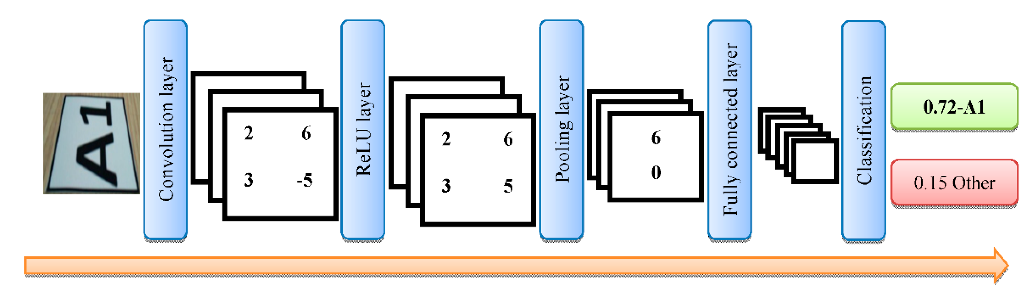
Deep learning is a method that can make decisions using data characteristics and reduce dependence on experts [
5]. CNN is a widely used type of deep-learning method. It is a multi-layered neural network model consisting of convolutional, rectified linear units (ReLUs), pooling, and fully connected layers [
6]. Camera images can be analyzed quickly by using deep-learning methods. The routes of vehicles used in production environments can be designed flexibly. The images of these designed routes can be easily obtained with vehicle cameras and determined using deep-learning models. Thus, vehicles can analyze routes and go to their destination without human intervention. Smolyansky et al. present a micro aerial vehicle system for outdoor environments such as forests based on a deep neural network called TrailNet [
7]. Wang et al. obtained road signs using a camera mounted onto an AGV. They applied these signals as input to a neural network they developed and performed the visual-based path tracking of the AGV [
8].
In the present study, an image processing and a deep-learning-based indoor positioning system are proposed to solve the real-time route tracking and collision problems of autonomous vehicles used in indoor production environments [
9,
10]. In the proposed system, a floor path model consisting of markers was developed for the ground. The markers used in the floor path model are formed from a combination of letters and numbers. Routes are created using these markers. First, the floor path model is sent as a vector to autonomous vehicles by a server. The target marker address is required for the vehicle to move. The routes to the destination address and the distances of these routes are calculated by the vehicle. The closest route to the destination is selected from among the calculated routes. If there is no other vehicle on the selected route within four marker route distances from the vehicle, the vehicle model is activated. If there is another vehicle on the selected route, the same checks are made for the other route closer to the target. If no empty route is found, the vehicle model is suspended. While the autonomous vehicle moves on the route, the images obtained from the camera mounted on the autonomous vehicle model (AVM) are processed with pre-processing image methods. These images are given as input to the CNN model trained using the transfer learning method. The network output is compared with the corresponding element of the target route vector to ensure that the autonomous vehicle model follows the route. If the route vector information of the network output is equal, the address information from other vehicles is checked. If the vehicle whose address information is received is four markers away from the relevant vehicle, the relevant vehicle waits; otherwise, it will continue. These processes continue until the vehicle reaches its destination. The floor path model and algorithm used the created routes, allowing the autonomous vehicle to reach its destination by following the most appropriate route without colliding with another vehicle.
The main contributions of our work can be summarized as follows:
We design a deep-learning-based floor path model for route tracking of autonomous vehicles.
It is a collision-free indoor positioning system for autonomous route tracking vehicles, based on the CNN deep-learning model.
A new floor road model and algorithm based on indoor positioning has been developed for autonomous vehicles.
The vehicles calculate all the routes to the target location in the floor path model and choose the shortest path and follow the route with high accuracy.
The experiments we have carried out confirmed the validity of our model.
The rest of this paper is structured as follows.
Section 2 summarizes the related works. In
Section 3, the subtitles of convolutional neural network, preparing the data sets, and obtaining the region of interest in the frame were presented under the materials and methods.
Section 4 describes the proposed the deep-learning-based floor path model for route tracking.
Section 5 presents experimental results.
Section 6 summarizes results and discuss the results of the study. Finally,
Section 7 provides a conclusion and proposes potential future works.
2. Related Work
In recent years, studies on the development of autonomous vehicles have been performed. Different problems are encountered in autonomous vehicles used in production environments. One of these problems is real-time route tracking. Another problem is that the vehicle moving on the route can collide with another vehicle. Some of the studies on autonomous vehicles have focused on route-tracking strategies. These strategies are important for automated guided vehicles (AGVs) used in production areas. Collision avoidance is a critical problem in the motion planning and control of AGVs [
11,
12]. A collision can occur when AGVs move in the same direction on the same road and in the opposite direction on the same road [
13]. Guney et al. designed a controller aimed at resolving motion conflicts between AGVs. They used the traditional right-handed two-way traffic system based on the motion characteristics of AGVs in the controller design. They prevented collisions by determining the right of way for AGVs that would encounter each other at an intersection [
14]. Zhao et al. proposed a dynamic resource reservation (DRR) based method that supports collision avoidance for AGVs. In this method, the layout is divided into square blocks of the same size. AGVs moving on each square shared their points. These source points were extracted from the guide paths in real time in the algorithm. The authors then took advantage of collision and crash prevention to make decisions for dynamic resource reservations. These two parameters allowed AGVs to travel without crashes while improving time efficiency. The simulation results in the study showed that the travel time was shortened between 11% and 28% [
15]. Guo et al. developed a path-planning model to avoid collisions for AGVs. The authors calculated the travel speed, run time, and collision distance parameters of the AGV relative to its minimum inhibition rate. They performed several experiments to compare the average blocking rate, wait time, and completion time of different AGVs; run time under different interactive protocols; and average blocking rate of different scale maps. As a result of the experiments, they showed that the acceleration control method could resolve the collision faster and reduce the secondary collision probability [
16].
AGVs follow a guidance system that contains the routing information in the environment. The guidance technologies used by AGVs are wire/inductive guidance, optical line guidance, magnetic tape guidance, laser navigation guidance, wireless sensor network guidance, vision guidance, barcode guidance, ultrasonic guidance, and GPS guidance [
17,
18,
19].
Murakami, K. used a time–space network to formulate AGV routing as a mixed-integer linear programming problem. In this network, he handled the routing of AGVs and materials separately. He experimentally tested his system [
20]. Lu et al. addressed the solution to the routing problem of AGVs using a deep-reinforcement-learning algorithm. They modeled the routing problem of AGVs as a Markov decision process and enabled real-time routing [
21]. Holovatenko et al. proposed a mathematical algorithm and tracking system, including energy efficiency, that creates and follows the desired route between two points on a specific map [
22]. Different studies based on autonomous driving methods of AGVs have been reported in the literature. The essential function of the autonomous driving method is machine vision. Some of the problems based on machine vision include floor path detection and strip marking detection [
23,
24,
25]. Bayona et al. used computer vision for line tracking with a camera mounted on a model AGV. The vehicle was mainly successful in following a straight line on the floor in their tests [
26]. Zhu et al. proposed a vehicle path tracking method that tracks the route by processing the image taken from the camera. They first applied a median filter to the image to clarify the road condition by reducing the picture’s noise and binarizing the image to reduce the computational complexity. They reduced image distortion and low path tracking accuracy issues [
27]. Lee et al. proposed a vision-based AGV navigation system that uses a camera to detect triangular markers placed at different locations on the floor. Using the image’s hue and saturation values to identify markers in an image and choosing markers of a specific size, they achieved a 98.8% recognition rate [
28]. Revilloud et al. developed a new strip detection and prediction algorithm. They used noise filters to improve the prediction of strip markers on the road. They detected the road in the image with 99.5% success using image processing and lane marking algorithms [
29]. Liu, Y. et al. proposed a robot motion trajectory control using the ant colony algorithm and machine vision. They have shown that the system developed with experimental research can make reasonable trajectory planning in complex environments [
30]. Lina et al. proposed a Kalman-based Single Shot Multi-Box Detector (K-SSD) target location strategy using a convolutional neural network (CNN) to improve position accuracy and mobile robot speed during automatic navigation. The experimental results showed that their proposed strategy increased the vehicle’s route detection and location accuracy in situations such as light differences and scene changes [
31]. Sun et al. used images from the camera in the vehicle to find the path of an autonomous vehicle in a warehouse. They trained the Faster Region-based CNN model with these images. The label and shelf feet in the image were identified using the trained CNN, inverse perspective mapping (IPM) algorithm, and the support vector machine (SVM) algorithm. They obtained a virtual guideline from the camera images using shelf legs and labels in specific areas. They did not use real-time image processing or navigation in their work [
32]. Ryota et al. developed an AGV transport system using deep-reinforced learning. They used map information for route planning in their transport system. They tested the validity of the method with the help of a simulator [
33].
4. Deep-Learning-Based Floor Path Model for Route Tracking
The floor path model designed for the proposed system in the present study consists of discrete cellular markers. The other model component is the vehicle with a camera following the routes in the proposed floor path model. Markers are a basic structure consisting of a letter and a number. The numbers to be added to the model are obtained from increasing and decreasing letter–number pairs. A letter is added first, and numbers up to nine are added after the letter. After A and 1 are added side by side, the value A1 to be written on the marker is obtained. This value also indicates the location address of the marker. The location of the vehicle can be determined using this address. For the subsequent marker address, the number 2 is added to the letter A. This process continues until the A9 marker address is obtained. Therefore, nine markers are obtained from one letter. There is no letter change as long as it continues in the same direction on the floor. A sequence of two letters and one number is used when no more single-character letters are left to create the markers. The floor path model is obtained using these markers.
While creating routes on the floor path model, increasing markers from the starting location to the target location are selected. Routes created from markers, including increasing and decreasing letter–number pairs, also constitute ascending or descending routes. One advantage of using ascending or descending markers is that when the autonomous vehicle is disconnected from the system, it can reach the starting point by following the markers in the descending direction. The first route created by this method is a vector containing markers A1, A2, A3, A4, A5, D1, and D2. The D1 marker address is used because the vehicle’s direction will change after the A5 address in this route vector. The routes are composed of increasing or decreasing marker vectors, enabling the vehicle model to follow these routes. Bold lines are drawn around the markers to facilitate the detection of the marker. Intersections are formed at a 90-degree angle. There are twenty-five centimeters between the markers.
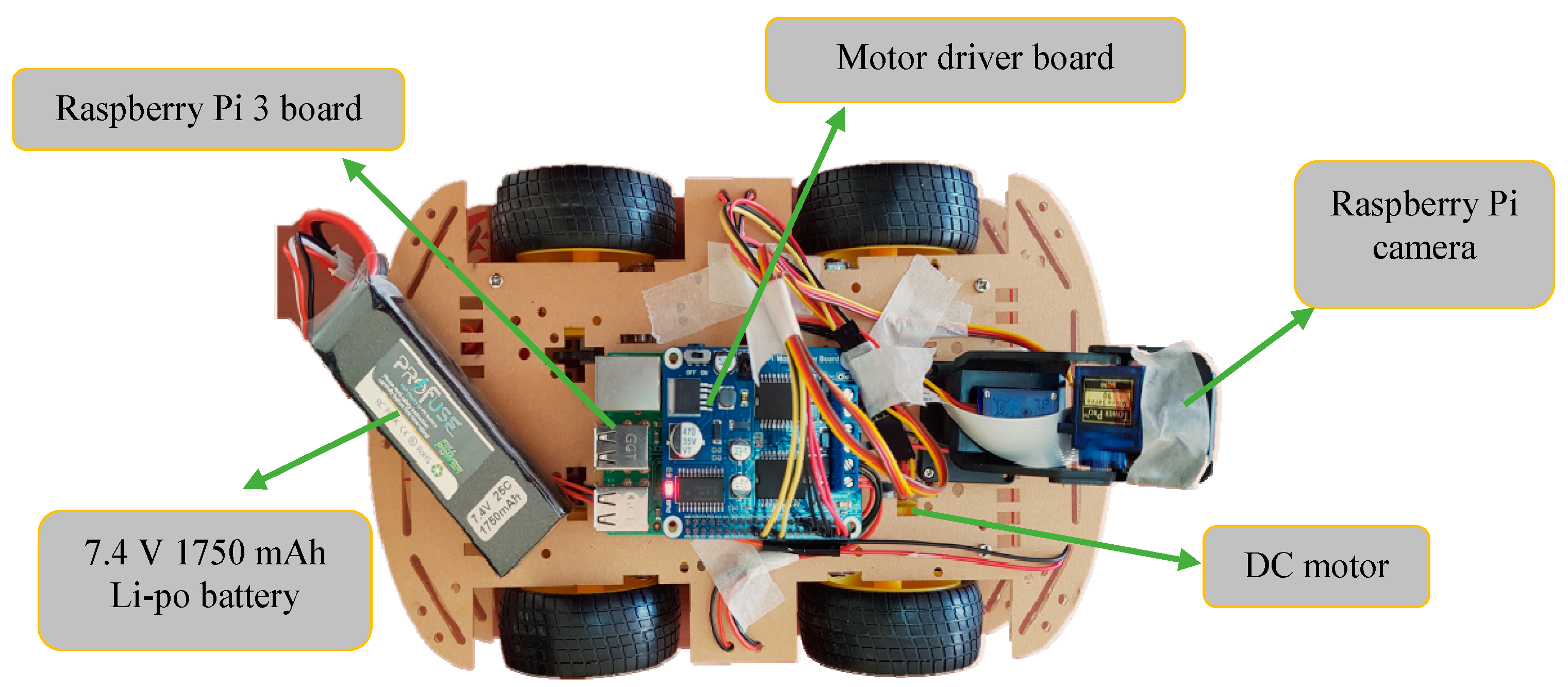
Special autonomous vehicles suitable for the proposed model were developed. A Raspberry Pi 3 board, Raspberry Pi motor driver board, 640 × 480 pixel color Raspberry Pi camera, and 7.4 V 1750 mAh Li-po battery were installed on the developed AVM. Furthermore, the AVM movement and the change in direction were controlled using several four direct current (DC) motors connected to the AVM wheels. The vehicle can drive at two different speeds. The camera on the vehicle has a single viewing angle and does not move left or right. The AVM used in the present study is shown in
Figure 4.
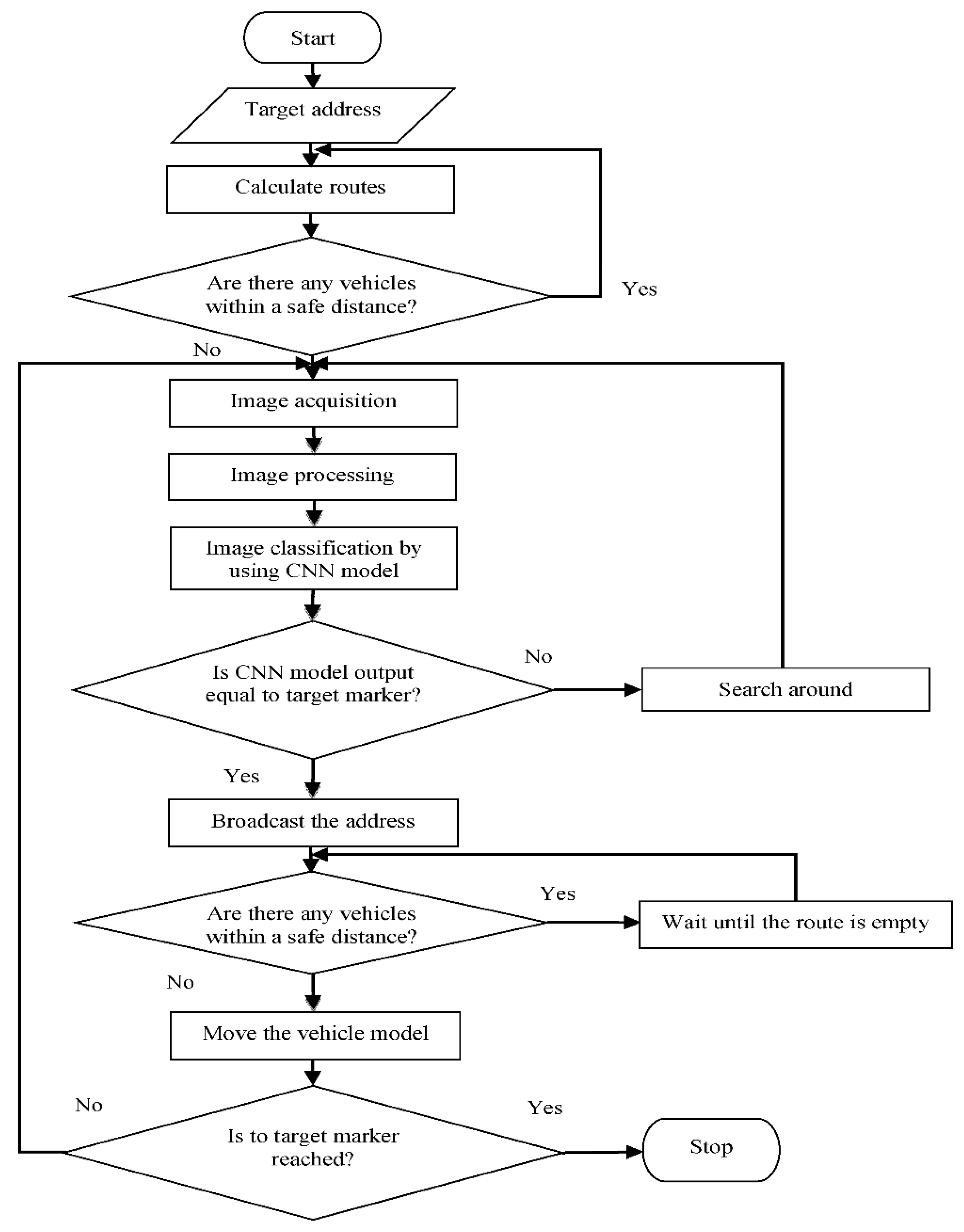
First, in the proposed system, the floor path model is sent as a vector to autonomous vehicles by a server. The target marker address is required for the vehicle to move, as shown in
Figure 5. The routes and approximate distances to the destination address are calculated by the vehicle. The closest route to the destination address is selected among the calculated routes. The destination vector of the selected route, which contains the markers to the destination, is created. The vehicle model is activated if there are no other vehicles on this route at least four marker distances from the selected vehicle. The four marker distances used were determined as the safe distance that prevents vehicles from colliding. Each vehicle broadcasts the last address information correctly classified by the deep-learning model on its route. If there is another vehicle on the selected route, the same checks are performed for the other route closer to the target. If no empty route is found, the vehicle model is suspended. One frame is taken per second from the video image obtained by the AVM camera in the image acquisition step. This image may contain more than one marker. The color image taken from the AVM camera is converted to a gray level image in the image processing step. By applying Gaussian blur, Canny edge detection, and Otsu algorithms to the gray level image, the frames of the distance markers in the image are blurred and the near ones are sharpened. Among these markers, the marker having the largest area is determined by comparing the area information of the markers in the image. This marker is cropped from the color image.
The cropped image is given as input to the pre-trained CNN model in the next algorithm step. The marker image classified by the CNN model is compared with the corresponding marker information in the target vector. Suppose the marker information is taken from the output of the network and this information is equal to the target vector marker information. In this case, the information as to whether there is another vehicle on the route is determined by using the address information sent by the vehicle moving on the route. If another vehicle is on the route, the new vehicle to follow the route waits to avoid a collision. If there is no other vehicle on the route, the vehicle moves along the route. If two vehicles have the same marker on their route, the movements of the vehicles are as follows: whichever vehicle is closer to the common marker, that vehicle continues to move on the route; the other vehicle continues to move when the address information of the common marker is not received.
In this way, collisions of vehicles are prevented. The markers in the target vector must be in ascending order for the model vehicle to move. If these two markers are different, the vehicle model turns to the right to see the images of the marker on the floor path and the operation of the system heads into the image acquisition step. The right turn of the vehicle model is important for the detection of other markers. These operations continue until the last marker in the target vector is reached. In the case of an error, the vehicle returns to its starting address using the markers in the vector.
The ascending order addressing method is used to calculate routes to the destination marker. The vehicles calculate routes and approximate distance to the target marker using incremental addressing from the vectors in the floor path model and keep these routes as vectors. The pseudo-code that calculates routes to the destination marker and their lengths is shown in Algorithm 1:
| Algorithm 1. The pseudo-code that calculates routes to the destination marker and their lengths. |
Let i = 0, k = 0, z = 0; RouteAll: array, RouteLocal:array
While I <= Vektor.Count
Let j = 0
Let V = Vector[i, j++]
RouteLocal[k++] = V
If V has sub vector
Add all SubVectors to RouteLocal
RouteAll[z++] = RouteLocal
i++
End While
Let Route: array, LengthRoute: array
i = 0, k = 0
While I <= RouteAll.Count
If RouteAll[i] Contains TagetMarker
Route[k] = RouteT[i]
LengthRoute[k] = Route[k].Count * Distance
i++
End While |
Here Vector contains all the markers in the floor path model received from the server. SubVector denotes subroutes going in different directions from a marker on the route. RouteAll shows all routes that will be created, while RouteLocal contains vectors and subroute vectors that will branch from a marker. Route addresses all routes to the target marker. LengthRoute is the length of each route to the destination marker and Distance indicates the distance between two markers.
Let the vehicle be given the F3 marker address as the target and the vehicle will go to the A3 marker position. The vehicle will calculate the route vectors to marker F3 as follows: the first route is A4, A5, A6, F1, F2, and F3. The second route is B1, B2, E1, E2, F2, and F3. The approximate length of each route is calculated by multiplying the number of markers by the distance between two markers. The route with the shorter distance is selected as the route to the destination. For a new scenario, the floor model has markers B1, B2, B3, C1, C2, C3, C4, D1, D2, D3, F1, F2, F3, F4, G1, G2, G3, H1. Let the vehicle be given the B1 marker address as the target and the vehicle will go to the G2 marker position. The vehicle will calculate the route vectors to marker G3 as follows: the first route is B2, B3, B4, B5, and G2. The second route is B2, B3, D1, D2, F1, F2, F3, F4, G1, and G2. The shortest route with markers B2, B3, B4, B5, and G2 will be selected.
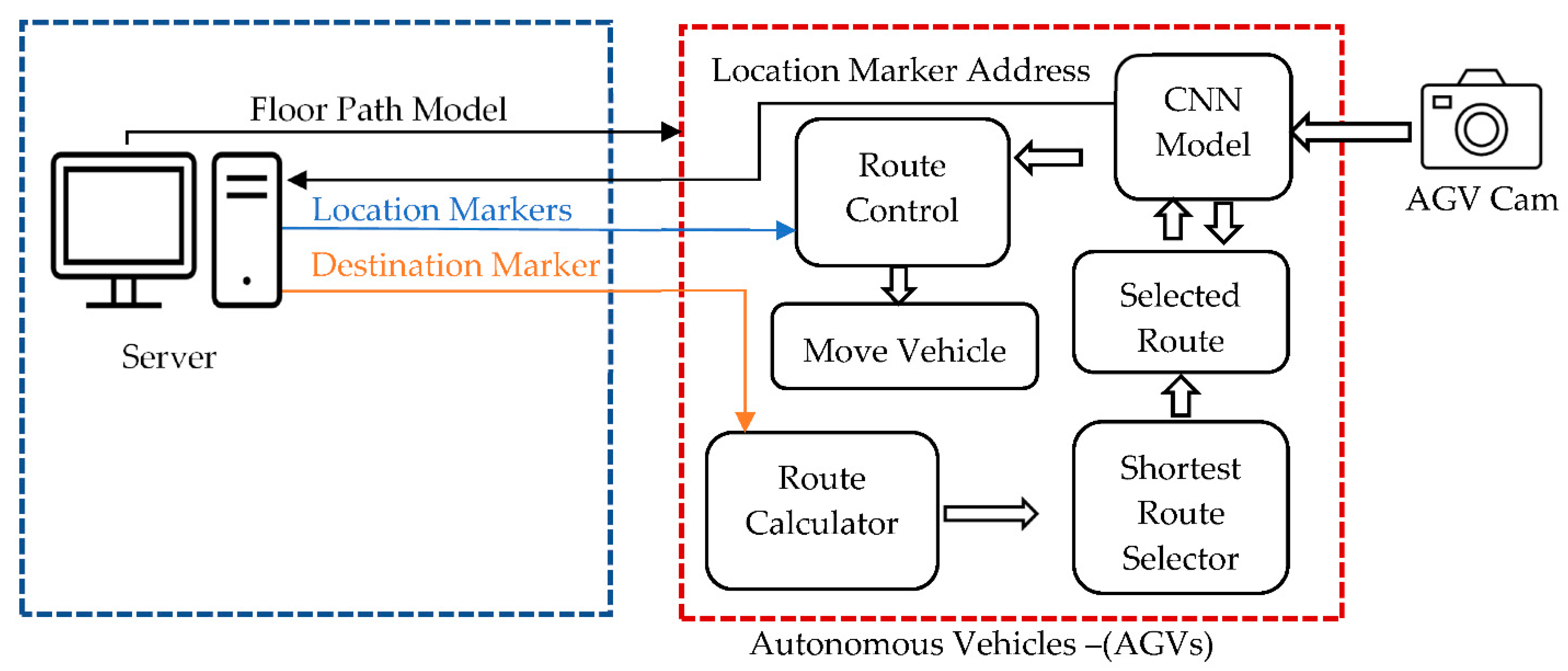
The working principle of the designed system can be briefly summarized as follows, shown in
Figure 6. All autonomous vehicles in an area act in communication with a central server. The server first sends the Floor Path Model to the vehicles as a vector. Then, the user or server gives the destination marker address to the vehicle that will move. The tool calculates all possible routes to this address and chooses the shortest one. On this selected route, the vehicle proceeds to reach the destination. While the vehicle moves on the route, it sends the last marker it reads to the server. Other autonomous vehicles know that there is a vehicle on that route by communication provided in this way.
5. Experimental Results
The performance of the deep-learning-based positioning system was tested by experiments. Different routes were created and used in the present study. For example, the first route consists of markers A1, A2, A3, A4, A5, D1, D2; the second route consists of markers A1, A2, A3, A4, A5, A6, F1, F2, F3, G1, G2; and the third route consists of markers A1 A2, A3, B1, B2, E1, E2, F2, F3, G1, G2. The studies were carried out for two different speed levels of the vehicle model for each route. The completion times of the routes and speed levels of the vehicle model are given in
Table 1.
The completion time of the route followed by the vehicle model varies according to the distance between the markers. The linear distance between the markers was taken as 25 cm. Images from the vehicle camera can be seen clearly by using the speed values given as 0.22 m/s and 0.27 m/s in
Table 1. However, when higher speeds are used, images from the vehicle camera become distorted.
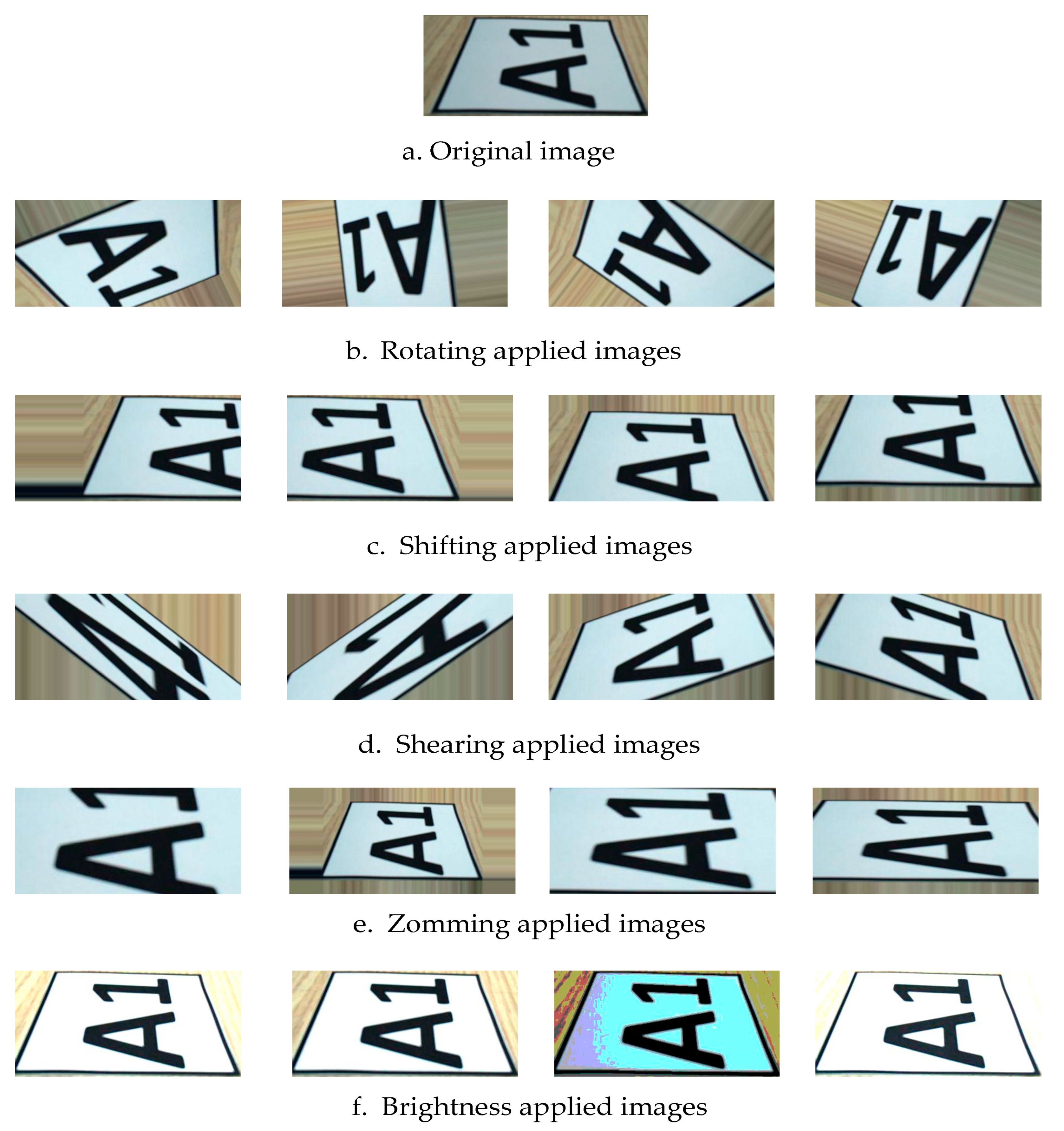
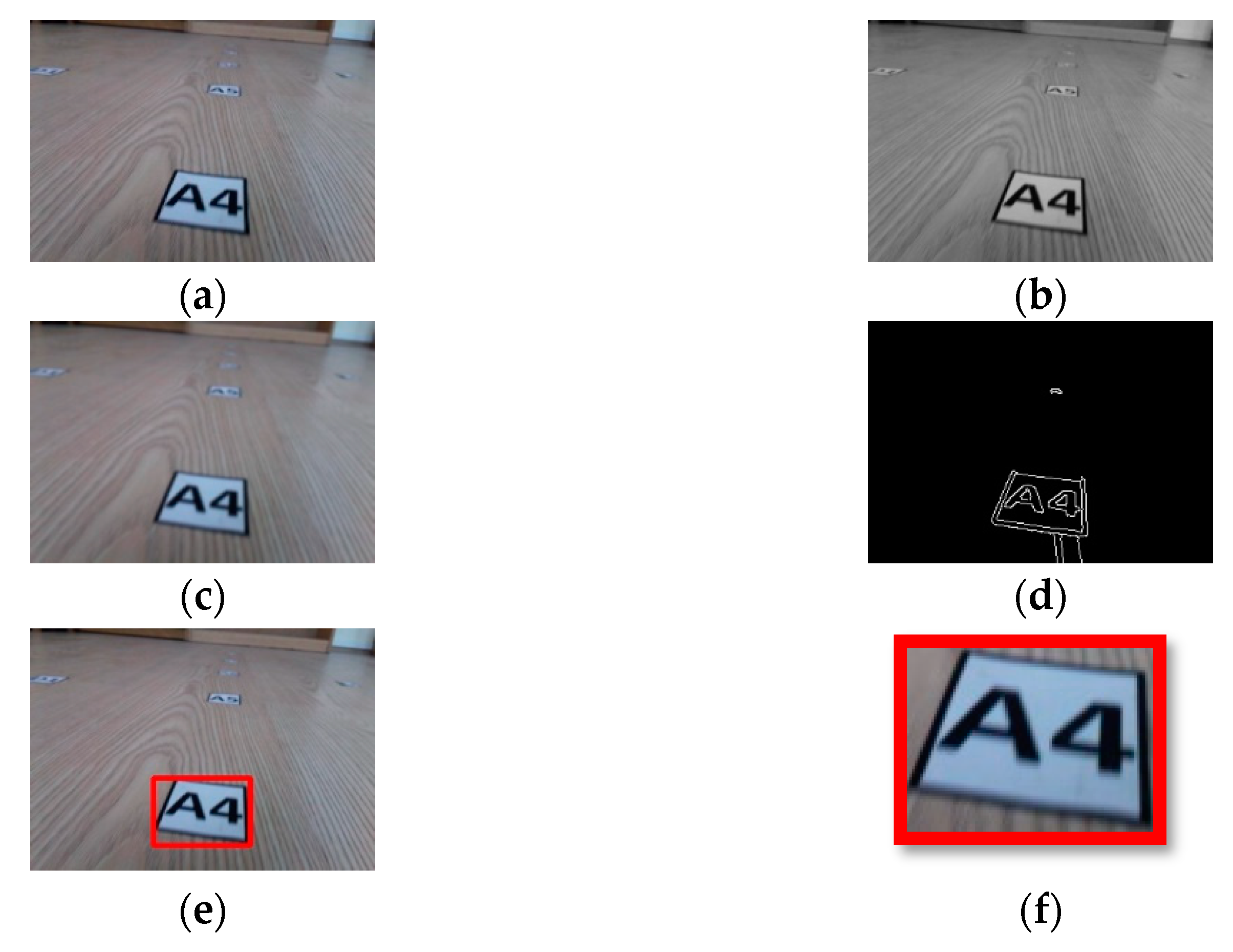
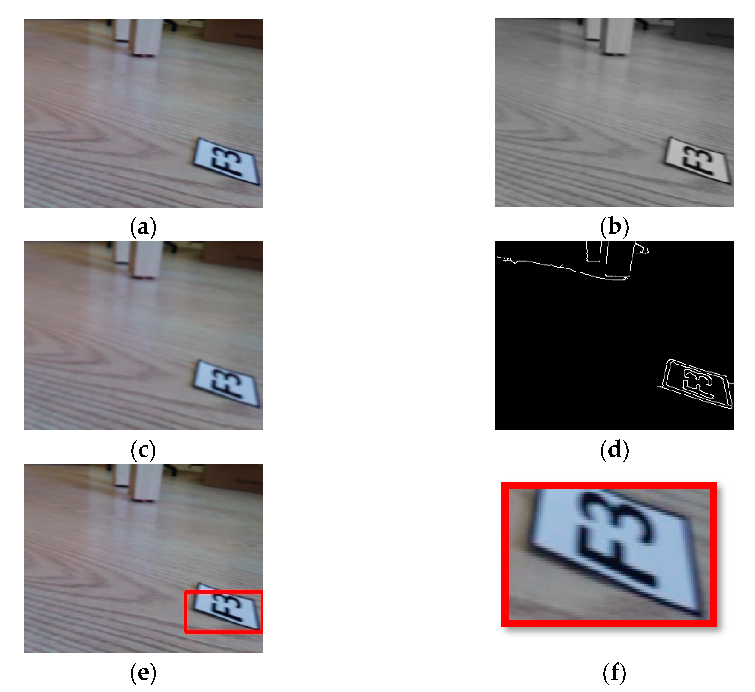
Images of markers A1, A2, A3, A4, A5, A6, B1, B2, D1, D2, E1, E2, F1, F2, F3, G1, G2 were augmented using the data augmentation methods. Of these data, 71% were reserved for training, 25% for validation, and 4% for testing. The CNN model was obtained using transfer learning and was trained with original and augmented images together. The images combined with the fully connected layer were classified into 17 different classes by the soft-max function. The steps to obtain the image of interest on the route by processing the images from the vehicle camera are shown in
Figure 7.
The application of the Otsu and Canny algorithms together with the image gave more successful results than the application of the Canny algorithm alone to obtain the markers in an image taken from the vehicle model camera.
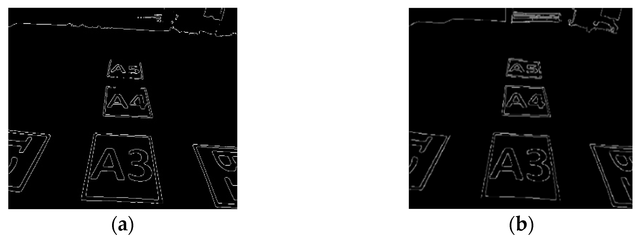
In the image where both algorithms are applied, there is more edge distortion at markers and objects far from the camera, and the success of detecting markers closer to the camera increases. Firstly, Gaussian blur was applied to the image in order to increase the distortion. As shown in
Figure 8, when images
Figure 8a,b are compared, it is clearly seen that edge distortions occur in
Figure 8a.
6. Results and Discussion
MobileNet is a model trained with an ImageNet dataset. The weights of this model were obtained by using transfer learning. The training set used in the study was different from the ImageNet dataset. For this reason, the weights of the model layers were updated with the new images used during the training. All layers were used in the MobileNet model except the last fully connected layers. The batch normalization layer was added to the classification layer in the model. Batch normalization acts as a regularizer, in some cases eliminating the need for Dropout [
43]. Batch normalization was used to reduce overfitting.
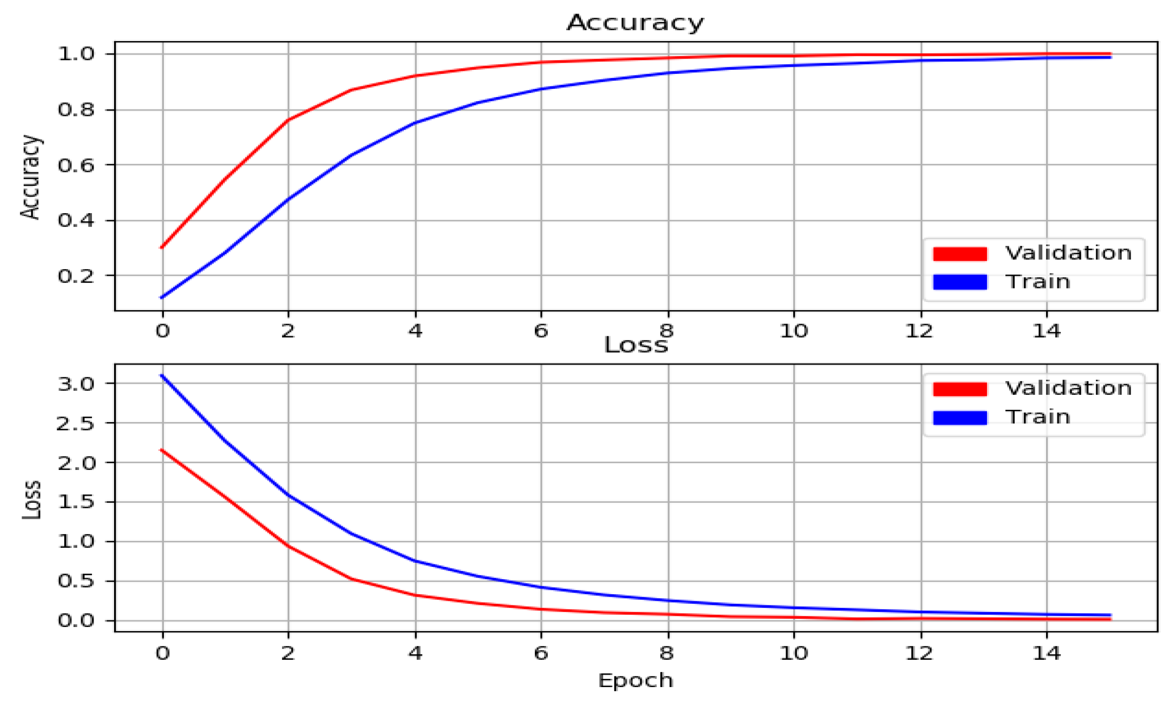
The low processor power in model vehicles accelerates the process of image processing. Therefore, the image size for model training was set to 160 × 160 × 3 pixels. The initial learning rate was 0.0001, and the loss function was selected as categorical cross-entropy. Because the number of classes was more than two, the categorical cross-entropy function was used. If the loss value cannot be reduced three times in a row with the determined learning rate, the learning rate is reduced by the specified delta value. The minimum delta value determined was 0.0001. There are classes that are similar to each other in the dataset. This causes problems in the performance graph while training the model. When the batch-size value is large, it takes more time for the model tool to process the data. When this value is small, the model learns the noises and moves away from generalization. Therefore, a mini-batch size of 32 was selected for each epoch at the end of the tests. Adam was used as the optimizer. Softmax was chosen because the activation function of the last layer consists of 17 classes. Model training was ended when the validation loss value was less than 0.009. Model training was completed in 16 epochs.
Training and loss graphics of the model are given in
Figure 9. It can be seen from the figure that the training loss and validation loss curves follow each other and progress at very close levels. To evaluate the performance of our model, we used the precision rate, recall rate, and F1-score metrics.
These performance metrics are given below:
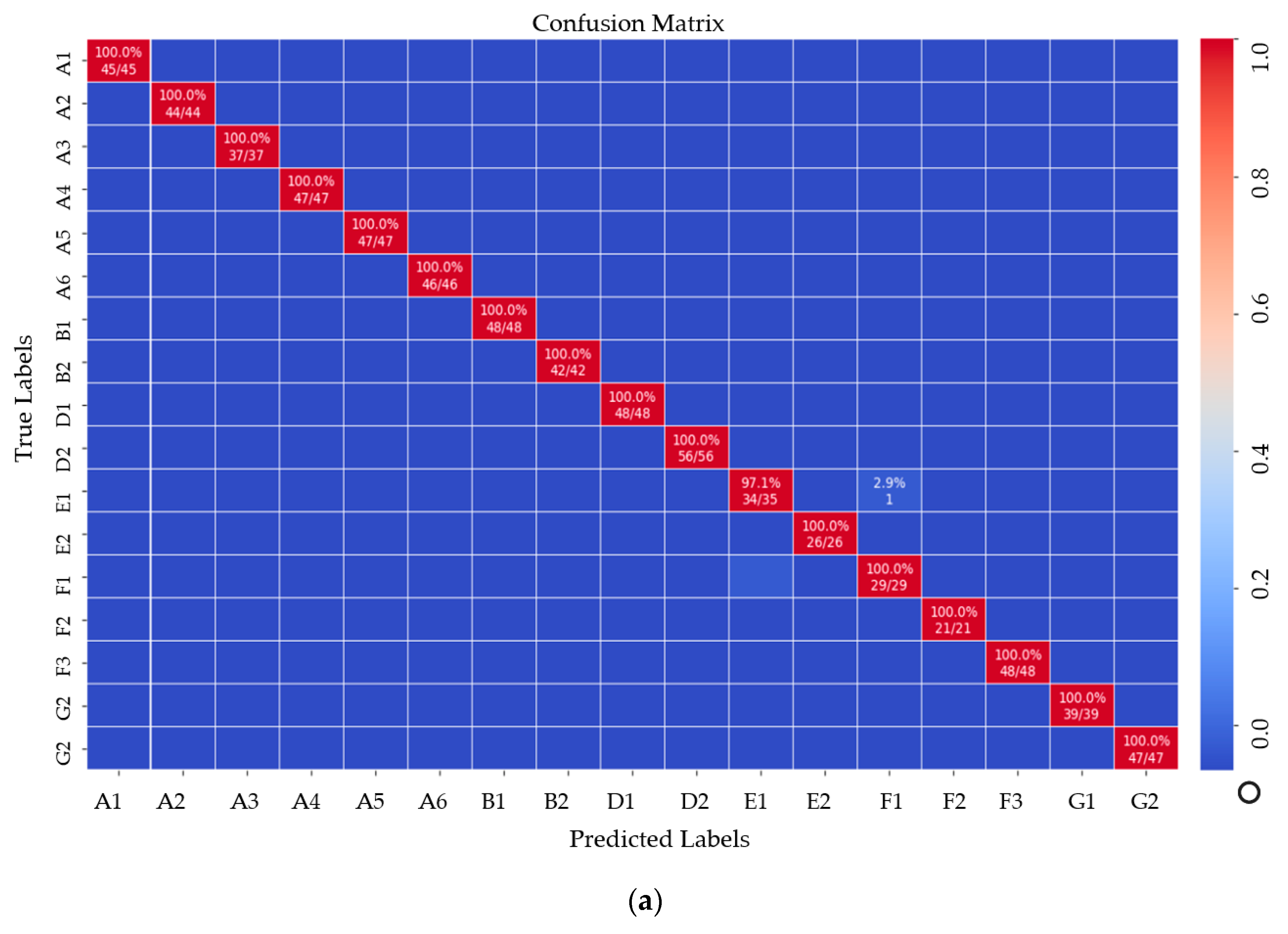
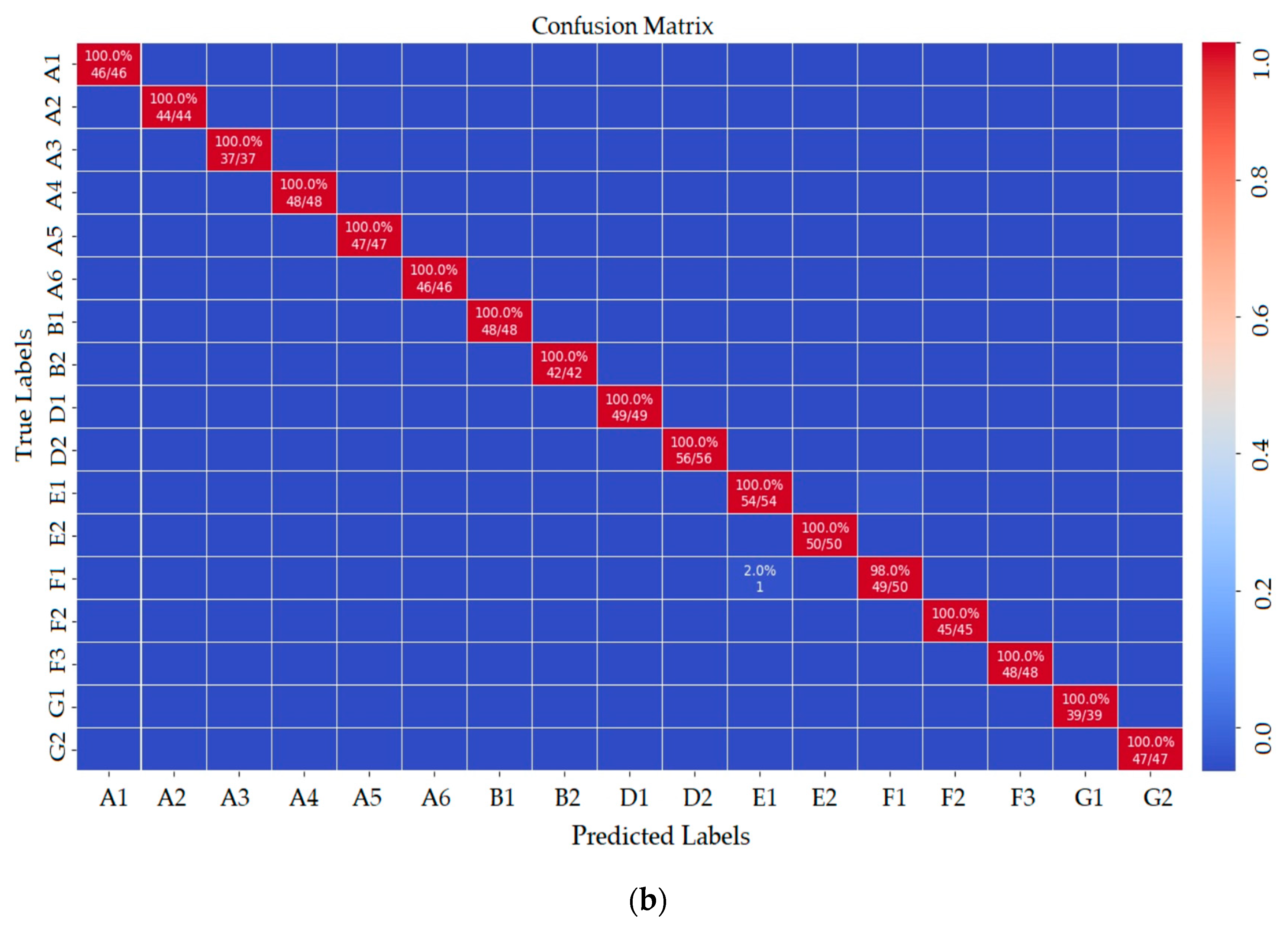
The precision metric shows how many of the values positively predicted by the model are positive. The recall metric shows how many of the values that the model should positively predict are positively estimated. Because there was more than one class in the dataset in the study, precision, recall, and F1-score metrics were also used besides the classification accuracy metric for model performance. It is seen that all other markers except the E1 marker were classified correctly in the confusion matrix shown in
Figure 10a. When the matrix was examined, it was seen that the marker that should be classified as E1 was incorrectly classified as F1. Thirty-four of the 35 E1 markers were correctly classified. This is because the E1 and F1 markers are similar. To test the trained deep-learning model, a total of 796 marker images, which were never given before, were entered as input to the model. As seen in
Figure 10b, the model classified the F1 marker image 49 times as F1 and once as E1.
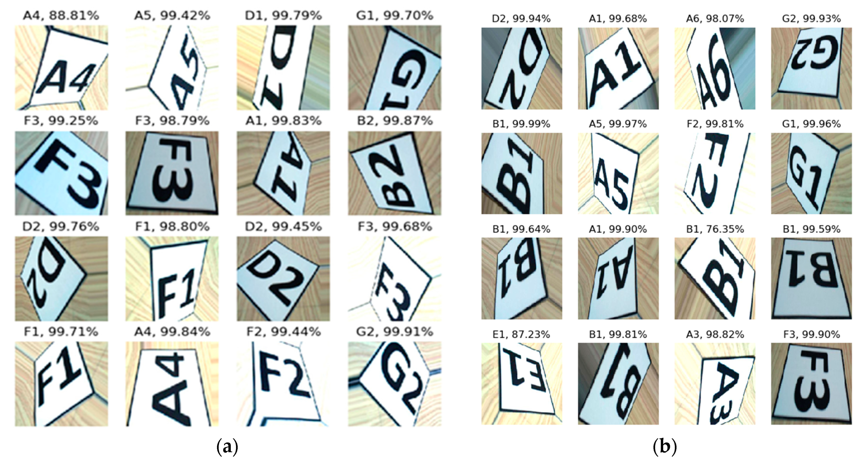
The results obtained when the test set images were applied to the trained model, which are shown in
Figure 11. It is seen here that the A4 image on the left has the lowest ratio of 88.81%, and the B1 image on the right has 76.35%. Both markers are correctly classified by the trained model. It is also seen that the model classifies all markers correctly. The performance metrics of the trained model are given in
Table 2. It can be seen in the table that marker E1 has the lowest value with a 0.97 recall metric value. It is seen that the F1 score value of the E1 marker is 0.99. The F1 marker has a 0.97 precision ratio and a 0.98 F1 score rate.
It can be seen from
Table 2 that the worst performance of the model is 97%. The average performance of each metric is 99.82%.
The ROI image obtained by pre-processing from the view from the AVM camera was given as input to the trained model. The latency times of the model to classify this image are given in
Table 3. It can be seen from the table that the average latency time is 0.01449 s.
7. Conclusions
Traditional floor path methods used in production areas have a limited number of road routes, which can cause traffic congestion and workload imbalance. In the present study, an indoor positioning system based on a floor path model and algorithm have been developed for autonomous vehicles. A floor path model consisting of markers was developed. All routes to a given destination on the floor path model are created using the dynamic route planner. The vehicle chooses the shortest alternative route with the least number of vehicles among these routes and goes to its destination without colliding with another vehicle. Markers on the floor path model can be detected with a low-resolution camera. Because the floor path model is created with increasing and decreasing markers, the vehicle model can easily follow a consecutive increasing or decreasing route. Traffic density can be minimized and workload can be balanced by using these alternative routes. Vehicles on the floor path model broadcast their marker address for all vehicles. If there is another vehicle on the vehicle’s route, it waits until there are at least four markers between the vehicles in the proposed algorithm. When the floor path model and algorithm are used, it is not allowed to have more than one vehicle at a marker address and collisions of vehicles are prevented. It was shown that it is possible to create multiple routes to the destination using the proposed floor path model.
When the results of the CNN model trained using transfer learning were examined, it was seen that 34 of the 35 E1 markers were correctly classified. The lowest recall metric value of 0.97 and an F1-score metric of 0.99 were obtained for the E1 marker containing 35 E1 marker images in the test set. The lowest precision metric of 0.97 and an F1-score metric of 0.98 were obtained for the F1 marker containing 29 F1 marker test images. When the test set images were applied to the trained CNN model, the lowest rate was classified as the A4 marker image with 88.81% and the highest rate with the G2 marker image with 99.91%. In addition, it was observed that the model correctly classified all the markers.
In the present study, by using the indoor positioning system, the route determined among many alternative routes was selected and followed. The results showed that the developed floor path model, algorithm, and deep-learning model can be used successfully both in a real production environment and in the service sector areas such as storage and healthcare.
One of the potential future works is that the experimentally designed and modeled pavement path model can be applied in real industrial environments. The camera was fixed in the autonomous vehicle used in the present study. Action cameras could be used in future studies.


