
ANN-Based Model for the Prediction of the Bond Strength between FRP and Concrete


Abstract
:
1. Introduction
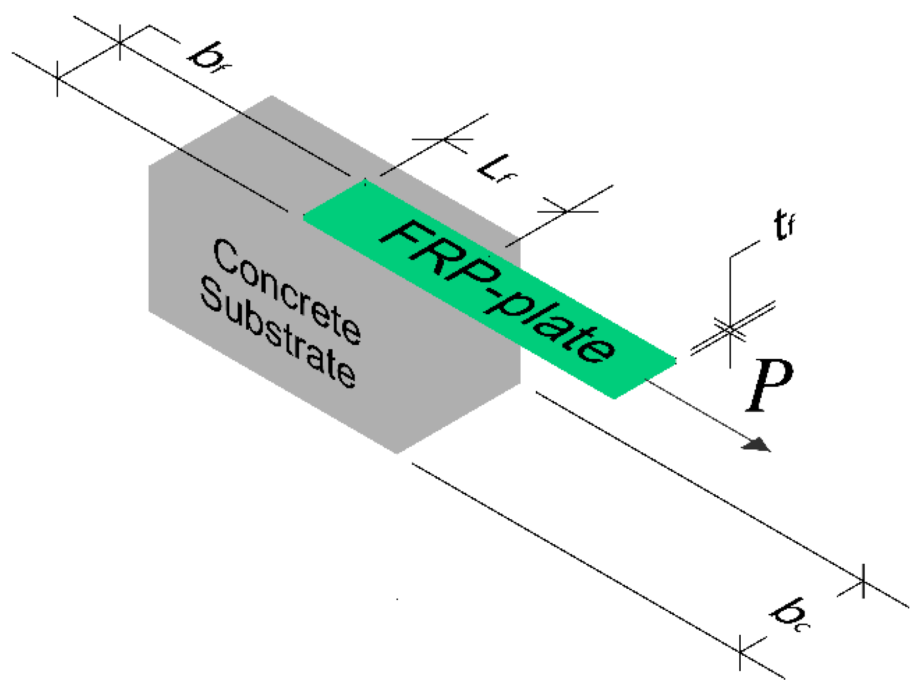
2. A Background of the Bond Behavior between FRP and Concrete Substrate
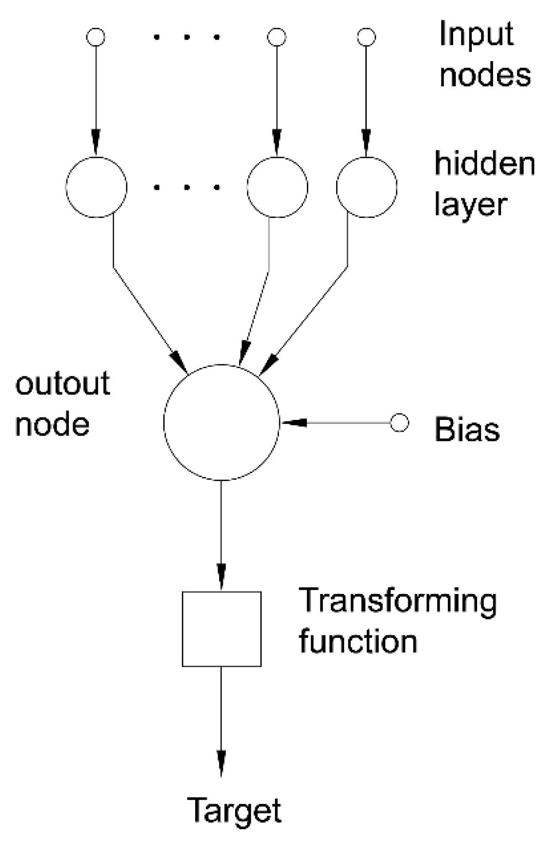
3. The Artificial Neural Networks (ANN)
- xi is the input data of the generic i-input-node;
- wi is the weight of a generic node in the hidden layer;
- b is the bias;
- y is the value of the output node;
- T is the target;
- K is a shape factor.
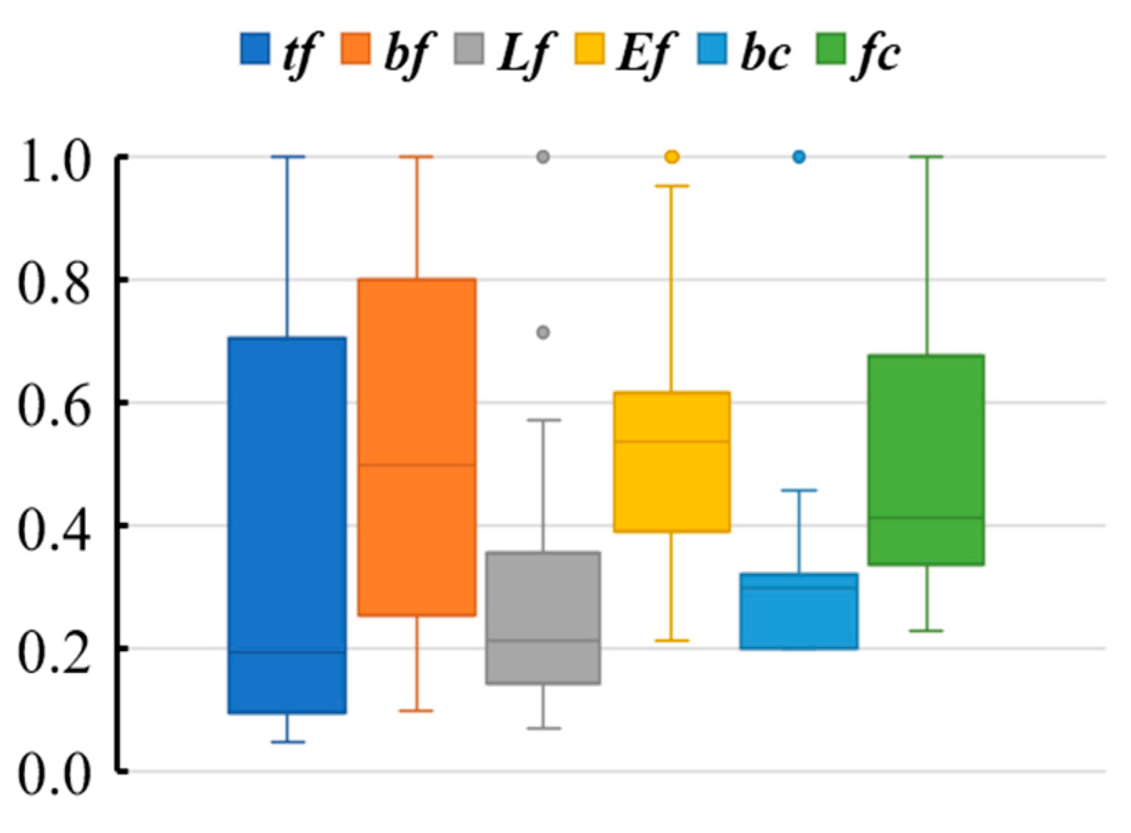
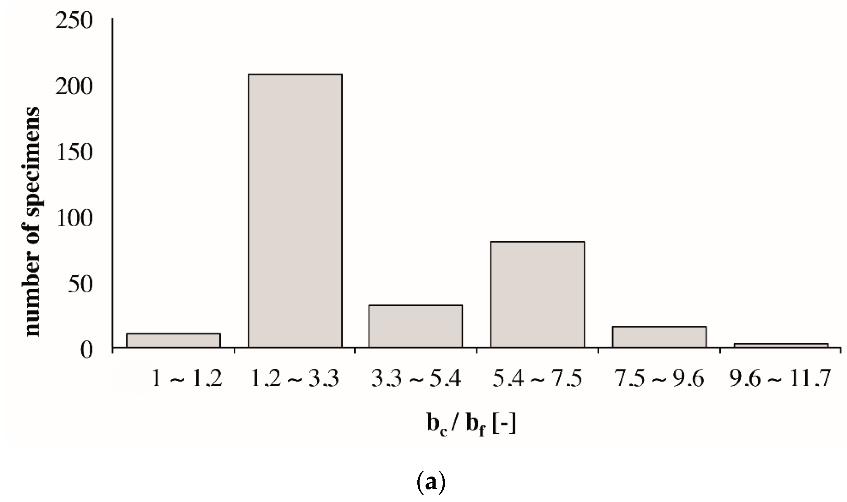
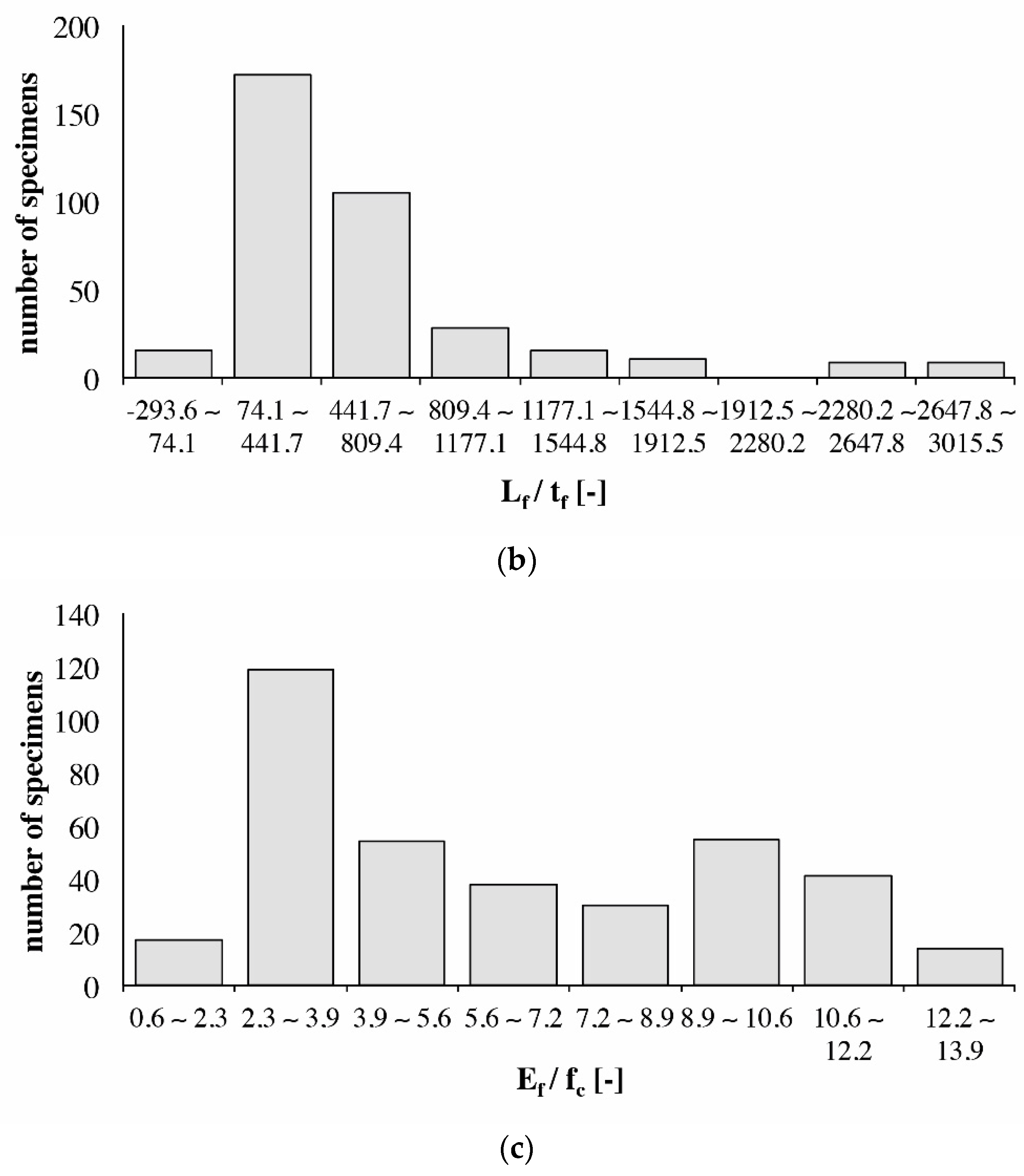
4. Experimental Database for the Formulation of the Theoretical Model
- tf, the thickness of the FRP sheet (mm);
- bf, the width of the FRP sheet (mm);
- Ef, the Young’s modulus of the FRP sheet (GPa);
- Lf, the bond length of the FRP sheet (mm);
- fc, the compressive strength of the concrete (MPa);
- bc, the width of the tested concrete element (mm).
5. ANN Proposed Model
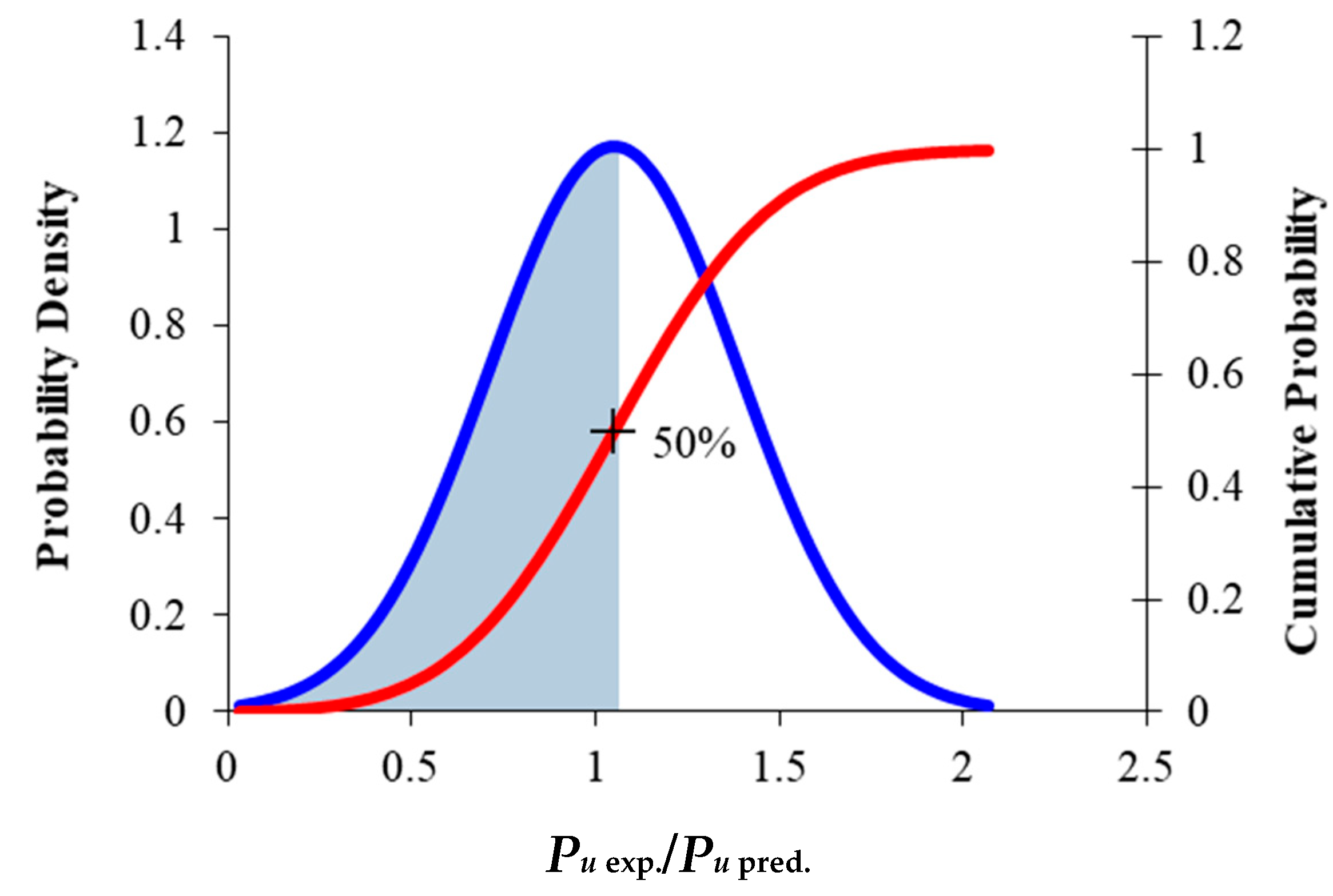
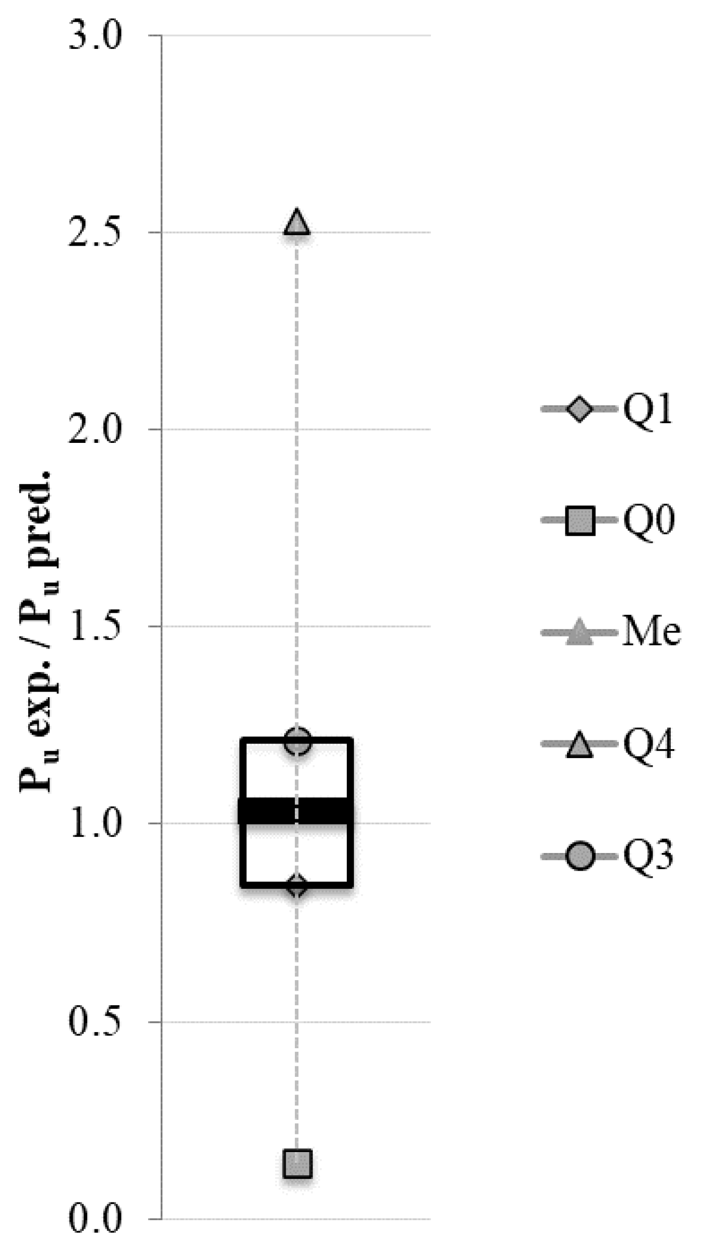
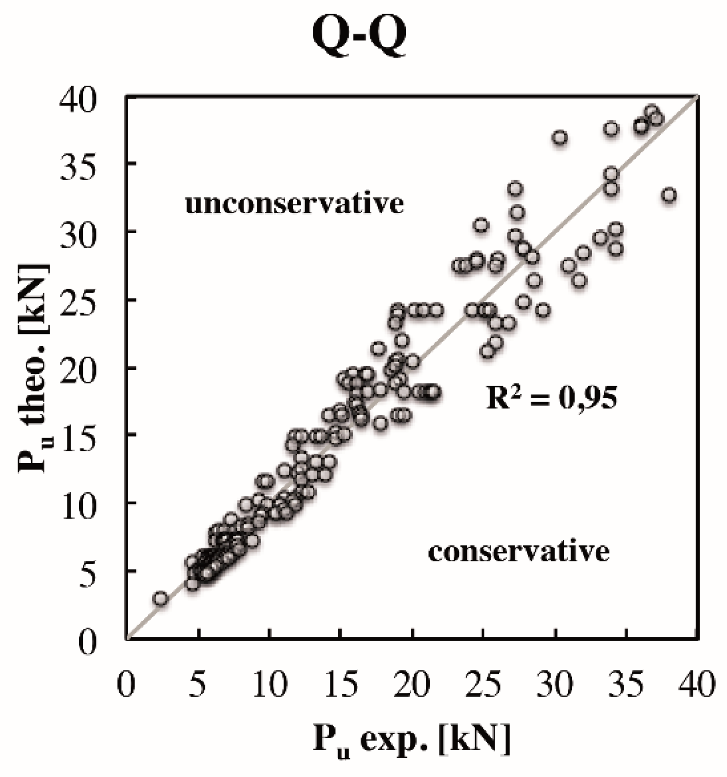
5.1. Model Evaluation
5.2. Robustness Analysis
- SE is the square error between the experimental and theoretical values;
- A is the SE higher response integer;
- n total number of respondents.
6. Comparison with Existing Analytical Models
- K > 0: the curve is defined leptokurtic, i.e., more “pointed” of a normal;
- K < 0: the curve is defined platykurtic, that is “flatter” than a normal;
- K = 0 the curve is defined normocurtica, i.e., “flat” as a normal.
- Mo is the mode.
- μ is the average value.
- σ is the standard deviator.
- n is the number of samples in the input database,
- i is the general sample,
- yi is the experimental value,
7. Conclusions
Author Contributions
Funding
Institutional Review Board Statement
Informed Consent Statement
Data Availability Statement
Conflicts of Interest
Appendix A

| References | Specimen Label | tf (mm) | bf (mm) | Lf (mm) | Ef (GPa) | bc (mm) | fc (MPa) | Pu (kN) |
|---|---|---|---|---|---|---|---|---|
| [47] | C1 | 1.016 | 25.4 | 76.2 | 108.478 | 228.6 | 36.1 | 8.462 |
| C2 | 1.016 | 25.4 | 76.2 | 108.478 | 228.6 | 47.1 | 9.931 | |
| C3 | 1.016 | 25.4 | 76.2 | 108.478 | 228.6 | 47.1 | 10.683 | |
| C4 | 1.016 | 25.4 | 76.2 | 108.478 | 228.6 | 47.1 | 10.683 | |
| C5 | 1.016 | 25.4 | 76.2 | 108.478 | 228.6 | 43.6 | 10.531 | |
| C7 | 1.016 | 25.4 | 76.2 | 108.478 | 228.6 | 43.6 | 9.61 | |
| C8 | 1.016 | 25.4 | 76.2 | 108.478 | 228.6 | 43.6 | 10.518 | |
| C9 | 1.016 | 25.4 | 76.2 | 108.478 | 228.6 | 43.6 | 11.199 | |
| C10 | 1.016 | 25.4 | 76.2 | 108.478 | 228.6 | 24 | 9.869 | |
| C11 | 1.016 | 25.4 | 76.2 | 108.478 | 228.6 | 28.9 | 9.343 | |
| C12 | 1.016 | 25.4 | 76.2 | 108.478 | 228.6 | 43.7 | 11.204 | |
| C13 | 1.016 | 25.4 | 76.2 | 108.478 | 228.6 | 36.4 | 8.094 | |
| C14 | 1.016 | 25.4 | 76.2 | 108.478 | 228.6 | 36.4 | 12.811 | |
| C15 | 1.016 | 25.4 | 76.2 | 108.478 | 228.6 | 36.4 | 11.917 | |
| C16 | 1.016 | 25.4 | 76.2 | 108.478 | 228.6 | 36.4 | 11.57 | |
| [48] | 1_11 | 0.167 | 40 | 100 | 230 | 100 | 28.88 | 8.75 |
| 1_12 | 0.167 | 40 | 100 | 230 | 100 | 26.66 | 8.85 | |
| 1_21 | 0.167 | 40 | 200 | 230 | 100 | 28.88 | 9.3 | |
| 1_22 | 0.167 | 40 | 200 | 230 | 100 | 26.66 | 8.5 | |
| 1_31 | 0.167 | 40 | 300 | 230 | 100 | 28.88 | 9.3 | |
| 1_32 | 0.167 | 40 | 300 | 230 | 100 | 26.66 | 8.3 | |
| 1_41 | 0.167 | 40 | 500 | 230 | 100 | 28.88 | 8.05 | |
| 1_42 | 0.167 | 40 | 500 | 230 | 100 | 28.88 | 8.05 | |
| 1_51 | 0.167 | 40 | 500 | 230 | 100 | 26.47 | 8.45 | |
| 1_52 | 0.167 | 40 | 500 | 230 | 100 | 26.47 | 7.3 | |
| 2_11 | 0.167 | 40 | 100 | 230 | 100 | 24.99 | 8.75 | |
| 2_12 | 0.167 | 40 | 100 | 230 | 100 | 24.99 | 8.85 | |
| 2_13 | 0.167 | 40 | 100 | 230 | 100 | 26.17 | 7.75 | |
| 2_14 | 0.167 | 40 | 100 | 230 | 100 | 26.17 | 7.65 | |
| 2_15 | 0.167 | 40 | 100 | 230 | 100 | 24.4 | 9 | |
| 2_21 | 0.167 | 40 | 100 | 230 | 100 | 24.99 | 12 | |
| 2_22 | 0.167 | 40 | 100 | 230 | 100 | 24.99 | 10.8 | |
| 2_31 | 0.167 | 40 | 100 | 230 | 100 | 24.99 | 12.65 | |
| 2_32 | 0.167 | 40 | 100 | 230 | 100 | 24.99 | 14.35 | |
| 2_41 | 0.167 | 40 | 100 | 230 | 100 | 24.4 | 11.55 | |
| 2_42 | 0.167 | 40 | 100 | 230 | 100 | 24.4 | 11 | |
| 2_51 | 0.167 | 40 | 100 | 230 | 100 | 26.17 | 9.85 | |
| 2_52 | 0.167 | 40 | 100 | 230 | 100 | 26.17 | 9.5 | |
| 2_61 | 0.167 | 40 | 100 | 230 | 100 | 26.17 | 8.8 | |
| 2_62 | 0.167 | 40 | 100 | 230 | 100 | 26.17 | 9.25 | |
| 2_71 | 0.167 | 40 | 100 | 230 | 100 | 26.17 | 7.65 | |
| 2_71 | 0.167 | 40 | 100 | 230 | 100 | 26.17 | 6.8 | |
| 2_81 | 0.167 | 40 | 100 | 230 | 100 | 49.97 | 7.75 | |
| 2_82 | 0.167 | 40 | 100 | 230 | 100 | 49.97 | 8.05 | |
| 2_91 | 0.167 | 40 | 100 | 230 | 100 | 24.4 | 6.75 | |
| 2_92 | 0.167 | 40 | 100 | 230 | 100 | 24.4 | 6.8 | |
| 2_101 | 0.167 | 40 | 100 | 230 | 100 | 24.99 | 7.7 | |
| 2_102 | 0.167 | 40 | 100 | 230 | 100 | 26.17 | 6.95 | |
| [49] | I-1 | 0.165 | 25 | 75 | 256 | 150 | 23 | 4.75 |
| I-2 | 0.165 | 25 | 85 | 256 | 150 | 23 | 5.69 | |
| I-3 | 0.165 | 25 | 95 | 256 | 150 | 23 | 5.76 | |
| I-4 | 0.165 | 25 | 95 | 256 | 150 | 23 | 5.76 | |
| I-5 | 0.165 | 25 | 95 | 256 | 150 | 23 | 6.17 | |
| I-6 | 0.165 | 25 | 115 | 256 | 150 | 23 | 5.96 | |
| I-7 | 0.165 | 25 | 145 | 256 | 150 | 23 | 5.95 | |
| I-8 | 0.165 | 25 | 190 | 256 | 150 | 23 | 6.68 | |
| I-9 | 0.165 | 25 | 190 | 256 | 150 | 23 | 6.35 | |
| I-10 | 0.165 | 25 | 95 | 256 | 150 | 23 | 6.17 | |
| I-11 | 0.165 | 25 | 75 | 256 | 150 | 23 | 5.72 | |
| I-12 | 0.165 | 25 | 85 | 256 | 150 | 23 | 6 | |
| I-13 | 0.165 | 25 | 95 | 256 | 150 | 23 | 6.14 | |
| I-14 | 0.165 | 25 | 115 | 256 | 150 | 23 | 6.1 | |
| I-15 | 0.165 | 25 | 145 | 256 | 150 | 23 | 6.27 | |
| I-16 | 0.165 | 25 | 190 | 256 | 150 | 23 | 7.03 | |
| II-1 | 0.165 | 25 | 95 | 256 | 150 | 22.9 | 5.2 | |
| II-2 | 0.165 | 25 | 95 | 256 | 150 | 22.9 | 6.75 | |
| II-3 | 0.165 | 25 | 95 | 256 | 150 | 22.9 | 5.51 | |
| II-4 | 0.165 | 25 | 190 | 256 | 150 | 22.9 | 7.02 | |
| II-5 | 0.165 | 25 | 190 | 256 | 150 | 22.9 | 7.07 | |
| II-6 | 0.165 | 25 | 190 | 256 | 150 | 22.9 | 6.98 | |
| III-1 | 0.165 | 25 | 100 | 256 | 150 | 27.1 | 5.94 | |
| III-2 | 0.165 | 50 | 100 | 256 | 150 | 27.1 | 11.66 | |
| III-3 | 0.165 | 75 | 100 | 256 | 150 | 27.1 | 14.63 | |
| III-4 | 0.165 | 100 | 100 | 256 | 150 | 27.1 | 19.07 | |
| III-7 | 1.27 | 25 | 100 | 225 | 150 | 27.1 | 4.78 | |
| IV-1 | 0.165 | 25 | 95 | 256 | 150 | 18.9 | 5.86 | |
| IV-2 | 0.165 | 25 | 95 | 256 | 150 | 18.9 | 5.9 | |
| IV-3 | 0.165 | 25 | 95 | 256 | 150 | 19.8 | 5.43 | |
| IV-4 | 0.165 | 25 | 95 | 256 | 150 | 19.8 | 5.76 | |
| IV-5 | 0.165 | 25 | 95 | 256 | 150 | 18.9 | 5 | |
| IV-6 | 0.165 | 25 | 95 | 256 | 150 | 19.8 | 7.08 | |
| IV-7 | 0.165 | 25 | 95 | 256 | 150 | 18.9 | 5.5 | |
| IV-8 | 0.165 | 25 | 95 | 256 | 150 | 19.8 | 5.93 | |
| IV-9 | 0.165 | 25 | 95 | 256 | 150 | 18.9 | 5.38 | |
| IV-10 | 0.165 | 25 | 95 | 256 | 150 | 19.8 | 6.6 | |
| IV-11 | 0.165 | 25 | 95 | 256 | 150 | 18.9 | 5.51 | |
| IV-12 | 0.165 | 25 | 95 | 256 | 150 | 19.8 | 5.67 | |
| IV-13 | 0.165 | 25 | 95 | 256 | 150 | 18.9 | 6.31 | |
| IV-14 | 0.165 | 25 | 95 | 256 | 150 | 19.8 | 6.19 | |
| V-1 | 0.165 | 15 | 95 | 256 | 150 | 21.1 | 3.81 | |
| V-2 | 0.165 | 15 | 95 | 256 | 150 | 21.1 | 4.41 | |
| V-3 | 0.165 | 25 | 95 | 256 | 150 | 21.1 | 6.26 | |
| V-4 | 0.165 | 50 | 95 | 256 | 150 | 21.1 | 12.22 | |
| V-5 | 0.165 | 75 | 95 | 256 | 150 | 21.1 | 14.29 | |
| V-6 | 0.165 | 100 | 95 | 256 | 150 | 21.1 | 15.58 | |
| VI-1 | 0.165 | 25 | 95 | 256 | 150 | 21.9 | 6.01 | |
| VI-2 | 0.165 | 25 | 95 | 256 | 150 | 21.9 | 5.85 | |
| VI-3 | 0.165 | 25 | 145 | 256 | 150 | 21.9 | 5.76 | |
| VI-4 | 0.165 | 25 | 145 | 256 | 150 | 21.9 | 5.73 | |
| VI-5 | 0.165 | 25 | 190 | 256 | 150 | 21.9 | 5.56 | |
| VI-6 | 0.165 | 25 | 190 | 256 | 150 | 21.9 | 5.58 | |
| VI-7 | 0.165 | 25 | 240 | 256 | 150 | 21.9 | 5.91 | |
| VI-8 | 0.165 | 25 | 240 | 256 | 150 | 21.9 | 5.05 | |
| VII-1 | 0.165 | 25 | 95 | 256 | 150 | 24.9 | 6.8 | |
| VII-2 | 0.165 | 25 | 95 | 256 | 150 | 24.9 | 6.62 | |
| VII-3 | 0.165 | 25 | 145 | 256 | 150 | 24.9 | 7.33 | |
| VII-4 | 0.165 | 25 | 145 | 256 | 150 | 24.9 | 6.49 | |
| VII-5 | 0.165 | 25 | 190 | 256 | 150 | 24.9 | 7.07 | |
| VII-6 | 0.165 | 25 | 190 | 256 | 150 | 24.9 | 7.44 | |
| VII-7 | 0.165 | 25 | 240 | 256 | 150 | 24.9 | 7.16 | |
| VII-8 | 0.165 | 25 | 240 | 256 | 150 | 24.9 | 6.24 | |
| [50] | I-3 | 0.825 | 50 | 100 | 110 | 200 | 17 | 11.64 |
| I-4 | 0.99 | 50 | 100 | 110 | 200 | 17 | 12.86 | |
| II-1 | 0.495 | 50 | 100 | 110 | 200 | 46.2 | 12.55 | |
| II-2 | 0.66 | 50 | 100 | 110 | 200 | 46.2 | 14.25 | |
| II-3 | 0.825 | 50 | 100 | 110 | 200 | 46.2 | 17.72 | |
| II-4 | 0.99 | 50 | 100 | 110 | 200 | 46.2 | 18.86 | |
| III-1 | 0.495 | 50 | 100 | 110 | 200 | 61.5 | 13.24 | |
| III-2 | 0.66 | 50 | 100 | 110 | 200 | 61.5 | 15.17 | |
| III-3 | 0.825 | 50 | 100 | 110 | 200 | 61.5 | 18.86 | |
| III-4 | 0.99 | 50 | 100 | 110 | 200 | 61.5 | 19.03 | |
| [51] | PG1-11 | 0.169 | 50 | 130 | 97 | 100 | 37.6 | 7.78 |
| PG1-12 | 0.169 | 50 | 130 | 97 | 100 | 37.6 | 9.19 | |
| PG1-1W1 | 0.169 | 75 | 130 | 97 | 100 | 37.6 | 10.11 | |
| PG1-1W2 | 0.169 | 75 | 130 | 97 | 100 | 37.6 | 13.95 | |
| PG1-1L11 | 0.169 | 50 | 100 | 97 | 100 | 37.6 | 6.87 | |
| PG1-1L12 | 0.169 | 50 | 100 | 97 | 100 | 37.6 | 9.2 | |
| PG1-1L21 | 0.169 | 50 | 70 | 97 | 100 | 37.6 | 6.46 | |
| PG1-1L22 | 0.169 | 50 | 70 | 97 | 100 | 37.6 | 6.66 | |
| PG1-21 | 0.338 | 50 | 130 | 97 | 100 | 37.6 | 10.49 | |
| PG1-22 | 0.338 | 50 | 130 | 97 | 100 | 37.6 | 11.43 | |
| PC1-1C1 | 0.111 | 50 | 130 | 235 | 100 | 37.6 | 9.97 | |
| PC1-1C2 | 0.111 | 50 | 130 | 235 | 100 | 37.6 | 9.19 | |
| NJ2 | 0.083 | 100 | 100 | 240 | 150 | 20.5 | 11 | |
| NJ3 | 0.083 | 100 | 150 | 240 | 150 | 20.5 | 11.25 | |
| NJ4 | 0.083 | 100 | 100 | 240 | 150 | 36.7 | 12.5 | |
| NJ5 | 0.083 | 100 | 150 | 240 | 150 | 36.7 | 12.25 | |
| NJ6 | 0.083 | 100 | 150 | 240 | 150 | 36.7 | 12.75 | |
| [52,53] | DLUT5-2G | 0.507 | 20 | 150 | 83.03 | 150 | 28.7 | 5.81 |
| DLUT5-5G | 0.507 | 50 | 150 | 83.03 | 150 | 28.7 | 10.6 | |
| DLUT5-7G | 0.507 | 80 | 150 | 83.03 | 150 | 28.7 | 18.23 | |
| DLUT30-1G | 0.507 | 20 | 100 | 83.03 | 150 | 45.3 | 4.63 | |
| DLUT30-2G | 0.507 | 20 | 150 | 83.03 | 150 | 45.3 | 5.77 | |
| DLUT30-3G | 0.507 | 50 | 60 | 83.03 | 150 | 45.3 | 9.42 | |
| DLUT30-4G | 0.507 | 50 | 100 | 83.03 | 150 | 45.3 | 11.03 | |
| DLUT30-6G | 0.507 | 50 | 150 | 83.03 | 150 | 45.3 | 11.8 | |
| DLUT30-7G | 0.507 | 80 | 100 | 83.03 | 150 | 45.3 | 14.65 | |
| DLUT30-8G | 0.507 | 80 | 150 | 83.03 | 150 | 45.3 | 16.44 | |
| DLUT50-1G | 0.507 | 20 | 100 | 83.03 | 150 | 55.5 | 5.99 | |
| DLUT50-2G | 0.507 | 20 | 150 | 83.03 | 150 | 55.5 | 5.9 | |
| DLUT50-4G | 0.507 | 50 | 100 | 83.03 | 150 | 55.5 | 9.84 | |
| DLUT50-5G | 0.507 | 50 | 150 | 83.03 | 150 | 55.5 | 12.28 | |
| DLUT50-6G | 0.507 | 80 | 100 | 83.03 | 150 | 55.5 | 14.02 | |
| DLUT50-7G | 0.507 | 80 | 150 | 83.03 | 150 | 55.5 | 16.71 | |
| DLUT15-2C | 0.33 | 20 | 150 | 207 | 150 | 28.7 | 5.48 | |
| DLUT15-5C | 0.33 | 50 | 150 | 207 | 150 | 28.7 | 10.02 | |
| DLUT15-7C | 0.33 | 80 | 150 | 207 | 150 | 28.7 | 19.27 | |
| DLUT30-1C | 0.33 | 20 | 100 | 207 | 150 | 45.3 | 5.54 | |
| DLUT30-2C | 0.33 | 20 | 150 | 207 | 150 | 45.3 | 4.61 | |
| DLUT30-4C | 0.33 | 50 | 100 | 207 | 150 | 45.3 | 11.08 | |
| DLUT30-5C | 0.33 | 50 | 100 | 207 | 150 | 45.3 | 16.1 | |
| DLUT30-6C | 0.33 | 50 | 150 | 207 | 150 | 45.3 | 21.71 | |
| DLUT30-7C | 0.33 | 80 | 100 | 207 | 150 | 45.3 | 22.64 | |
| DLUT50-1C | 0.33 | 20 | 100 | 207 | 150 | 55.5 | 5.78 | |
| DLUT50-4C | 0.33 | 50 | 100 | 207 | 150 | 55.5 | 12.95 | |
| DLUT50-5C | 0.33 | 50 | 150 | 207 | 150 | 55.5 | 16.72 | |
| DLUT50-6C | 0.33 | 80 | 100 | 207 | 150 | 55.5 | 16.24 | |
| DLUT50-7C | 0.33 | 80 | 150 | 207 | 150 | 55.5 | 22.8 | |
| [54] | Ueda_A1 | 0.11 | 50 | 75 | 230 | 100 | 29.74 | 6.25 |
| Ueda_A2 | 0.11 | 50 | 150 | 230 | 100 | 52.31 | 9.2 | |
| Ueda_A3 | 0.11 | 50 | 300 | 230 | 100 | 52.31 | 11.95 | |
| Ueda_A4 | 0.22 | 50 | 75 | 230 | 100 | 55.51 | 10 | |
| Ueda_A5 | 0.11 | 50 | 150 | 230 | 100 | 54.36 | 7.3 | |
| Ueda_A6 | 0.165 | 50 | 65 | 372 | 100 | 54.36 | 9.55 | |
| Ueda_A7 | 0.22 | 50 | 150 | 230 | 100 | 54.75 | 16.25 | |
| Ueda_A8 | 0.11 | 50 | 700 | 230 | 100 | 54.75 | 11 | |
| Ueda_A9 | 0.11 | 50 | 150 | 230 | 100 | 51.03 | 10 | |
| Ueda_A10 | 0.11 | 10 | 150 | 230 | 100 | 30.51 | 2.4 | |
| Ueda_A11 | 0.11 | 20 | 150 | 230 | 100 | 30.51 | 5.35 | |
| Ueda_A12 | 0.33 | 20 | 150 | 230 | 100 | 30.51 | 9.25 | |
| Ueda_A13 | 0.55 | 20 | 150 | 230 | 100 | 31.67 | 11.75 | |
| Ueda_B1 | 0.11 | 100 | 200 | 230 | 500 | 31.67 | 20.6 | |
| Ueda_B2 | 0.33 | 100 | 200 | 230 | 500 | 52.44 | 38 | |
| Ueda_B3 | 0.33 | 100 | 200 | 230 | 500 | 58.85 | 34 | |
| [55] | D-CFS-150-30 a | 0.083 | 100 | 300 | 230 | 100 | 58.85 | 12.2 |
| D-CFS-150-30 b | 0.083 | 100 | 300 | 230 | 100 | 73.85 | 11.8 | |
| D-CFS-150-30 c | 0.083 | 100 | 300 | 230 | 100 | 73.85 | 12.25 | |
| D-CFS-300-30 a | 0.167 | 100 | 300 | 230 | 100 | 73.85 | 18.9 | |
| D-CFS-300-30 b | 0.167 | 100 | 300 | 230 | 100 | 73.85 | 16.95 | |
| D-CFS-300-30 c | 0.167 | 100 | 300 | 230 | 100 | 73.85 | 16.65 | |
| D-CFS-600-30 a | 0.333 | 100 | 300 | 230 | 100 | 73.85 | 25.65 | |
| D-CFS-600-30 b | 0.333 | 100 | 300 | 230 | 100 | 73.85 | 25.35 | |
| D-CFS-600-30 c | 0.333 | 100 | 300 | 230 | 100 | 73.85 | 27.25 | |
| D-CFM-300-30 a | 0.167 | 100 | 300 | 390 | 100 | 73.85 | 19.5 | |
| D-CFM-300-30 b | 0.167 | 100 | 300 | 390 | 100 | 73.85 | 19.5 | |
| S-CFS-400-25 a | 0.222 | 40 | 250 | 230 | 100 | 73.85 | 15.4 | |
| S-CFS-400-25 b | 0.222 | 40 | 250 | 230 | 100 | 73.85 | 13.9 | |
| S-CFS-400-25 c | 0.222 | 40 | 250 | 230 | 100 | 73.85 | 13 | |
| S-CFM-300-25 a | 0.167 | 40 | 250 | 390 | 100 | 73.85 | 12 | |
| S-CFM-300-25 b | 0.167 | 40 | 250 | 390 | 100 | 73.85 | 11.9 | |
| S-CFM-900-25 a | 0.5 | 40 | 250 | 390 | 100 | 73.85 | 25.9 | |
| S-CFM-900-25 b | 0.5 | 40 | 250 | 390 | 100 | 73.85 | 23.4 | |
| S-CFM-900-25 c | 0.5 | 40 | 250 | 390 | 100 | 73.85 | 23.7 | |
| [56] | C165-100 | 1.2 | 50 | 100 | 165 | 100 | 29.7 | 18.25 |
| C165-130 | 1.2 | 50 | 130 | 165 | 100 | 29.7 | 24.5 | |
| C165-150 | 1.2 | 50 | 150 | 165 | 100 | 29.7 | 28.44 | |
| C165-175 | 1.2 | 50 | 175 | 165 | 100 | 29.7 | 32 | |
| C165-200 | 1.2 | 50 | 200 | 165 | 100 | 29.7 | 34.22 | |
| C165-250 | 1.2 | 50 | 250 | 165 | 100 | 29.7 | 33.14 | |
| C165-300 | 1.2 | 50 | 300 | 165 | 100 | 29.7 | 34.24 | |
| CFRP-C210 | 1.2 | 50 | 150 | 210 | 100 | 35.8 | 30.4 | |
| C210-180 | 1.2 | 50 | 180 | 210 | 100 | 35.8 | 34 | |
| C210-190 | 1.2 | 50 | 190 | 210 | 100 | 35.8 | 36 | |
| C210-200 | 1.2 | 50 | 200 | 210 | 100 | 35.8 | 36.02 | |
| C210-230 | 1.2 | 50 | 230 | 210 | 100 | 35.8 | 37.02 | |
| C210-255 | 1.2 | 50 | 255 | 210 | 100 | 35.8 | 36.8 | |
| CFRP-C300 | 1.2 | 50 | 160 | 300 | 100 | 29.7 | 38.02 | |
| C300-180 | 1.2 | 50 | 180 | 300 | 100 | 29.7 | 41.15 | |
| C300-200 | 1.2 | 50 | 200 | 300 | 100 | 29.7 | 46.35 | |
| C300-250 | 1.2 | 50 | 250 | 300 | 100 | 29.7 | 45.5 | |
| C300-300 | 1.2 | 50 | 300 | 300 | 100 | 29.7 | 45.95 | |
| [57] | - | 1.4 | 10 | 50 | 152.2 | 200 | 30 | 5.15 |
| - | 1.4 | 10 | 100 | 152.2 | 200 | 30 | 7.55 | |
| - | 1.4 | 10 | 150 | 152.2 | 200 | 30 | 7.7 | |
| - | 1.4 | 10 | 200 | 152.2 | 200 | 30 | 7.9 | |
| - | 1.4 | 10 | 250 | 152.2 | 200 | 30 | 6.25 | |
| - | 1.4 | 10 | 300 | 152.2 | 200 | 30 | 7.58 | |
| - | 1.4 | 10 | 50 | 152.2 | 200 | 40 | 5.1 | |
| - | 1.4 | 10 | 100 | 152.2 | 200 | 40 | 6.85 | |
| - | 1.4 | 10 | 150 | 152.2 | 200 | 40 | 6.35 | |
| - | 1.4 | 10 | 200 | 152.2 | 200 | 40 | 6.95 | |
| - | 1.4 | 10 | 250 | 152.2 | 200 | 40 | 6.8 | |
| - | 1.4 | 10 | 300 | 152.2 | 200 | 40 | 6.4 | |
| - | 1.4 | 10 | 50 | 152.2 | 200 | 50 | 4.55 | |
| - | 1.4 | 10 | 100 | 152.2 | 200 | 50 | 7.1 | |
| - | 1.4 | 10 | 150 | 152.2 | 200 | 50 | 7.78 | |
| - | 1.4 | 10 | 200 | 152.2 | 200 | 50 | 7.65 | |
| - | 1.4 | 10 | 250 | 152.2 | 200 | 50 | 6.8 | |
| - | 1.4 | 10 | 300 | 152.2 | 200 | 50 | 7.25 | |
| - | 1.4 | 30 | 50 | 152.2 | 200 | 30 | 9.3 | |
| - | 1.4 | 30 | 100 | 152.2 | 200 | 30 | 16.25 | |
| - | 1.4 | 30 | 150 | 152.2 | 200 | 30 | 16.2 | |
| - | 1.4 | 30 | 200 | 152.2 | 200 | 30 | 22.1 | |
| - | 1.4 | 30 | 250 | 152.2 | 200 | 30 | 15.6 | |
| - | 1.4 | 30 | 300 | 152.2 | 200 | 30 | 15.85 | |
| - | 1.4 | 30 | 50 | 152.2 | 200 | 40 | 9.15 | |
| - | 1.4 | 30 | 100 | 152.2 | 200 | 40 | 14.9 | |
| - | 1.4 | 30 | 150 | 152.2 | 200 | 40 | 16.05 | |
| - | 1.4 | 30 | 200 | 152.2 | 200 | 40 | 16.15 | |
| - | 1.4 | 30 | 250 | 152.2 | 200 | 40 | 16.11 | |
| - | 1.4 | 30 | 300 | 152.2 | 200 | 40 | 16.9 | |
| - | 1.4 | 30 | 100 | 152.2 | 200 | 50 | 17.8 | |
| - | 1.4 | 30 | 150 | 152.2 | 200 | 50 | 15.22 | |
| - | 1.4 | 30 | 200 | 152.2 | 200 | 50 | 18.5 | |
| - | 1.4 | 30 | 250 | 152.2 | 200 | 50 | 19 | |
| - | 1.4 | 30 | 300 | 152.2 | 200 | 50 | 17.71 | |
| - | 1.4 | 50 | 50 | 152.2 | 200 | 30 | 13.3 | |
| - | 1.4 | 50 | 100 | 152.2 | 200 | 30 | 26 | |
| - | 1.4 | 50 | 150 | 152.2 | 200 | 30 | 27.8 | |
| - | 1.4 | 50 | 200 | 152.2 | 200 | 30 | 27.2 | |
| - | 1.4 | 50 | 250 | 152.2 | 200 | 30 | 24.84 | |
| - | 1.4 | 50 | 300 | 152.2 | 200 | 30 | 23 | |
| - | 1.4 | 50 | 100 | 152.2 | 200 | 40 | 24.5 | |
| - | 1.4 | 50 | 150 | 152.2 | 200 | 40 | 27.75 | |
| - | 1.4 | 50 | 200 | 152.2 | 200 | 40 | 19.3 | |
| - | 1.4 | 50 | 250 | 152.2 | 200 | 40 | 21.9 | |
| - | 1.4 | 50 | 300 | 152.2 | 200 | 40 | 27.3 | |
| - | 1.4 | 50 | 100 | 152.2 | 200 | 50 | 16 | |
| - | 1.4 | 50 | 150 | 152.2 | 200 | 50 | 21.25 | |
| - | 1.4 | 50 | 200 | 152.2 | 200 | 50 | 25 | |
| - | 1.4 | 50 | 250 | 152.2 | 200 | 50 | 24.9 | |
| - | 1.4 | 50 | 300 | 152.2 | 200 | 50 | 34 | |
| [58] | T1a | 0.352 | 100 | 60 | 209 | 140 | 55.6 | 20 |
| T1b | 0.352 | 100 | 60 | 209 | 140 | 55.6 | 18.8 | |
| T2a | 0.352 | 100 | 80 | 209 | 140 | 55.6 | 25.8 | |
| T2b | 0.352 | 100 | 80 | 209 | 140 | 55.6 | 25.2 | |
| T3a | 0.352 | 100 | 100 | 209 | 140 | 55.6 | 25.8 | |
| T3b | 0.352 | 100 | 100 | 209 | 140 | 55.6 | 27.3 | |
| T4a | 0.352 | 100 | 140 | 209 | 140 | 55.6 | 26.7 | |
| T4b | 0.352 | 100 | 140 | 209 | 140 | 55.6 | 25.9 | |
| T5a | 0.352 | 100 | 180 | 209 | 140 | 55.6 | 27.8 | |
| T5b | 0.352 | 100 | 180 | 209 | 140 | 55.6 | 31.7 | |
| T6a | 0.352 | 100 | 220 | 209 | 140 | 55.6 | 31.7 | |
| T6b | 0.352 | 100 | 220 | 209 | 140 | 55.6 | 28.6 | |
| T7a | 0.352 | 100 | 100 | 209 | 140 | 55.6 | 33 | |
| T7b | 0.352 | 100 | 100 | 209 | 140 | 55.6 | 26.9 | |
| T8a | 0.352 | 100 | 100 | 209 | 140 | 55.6 | 28.5 | |
| T8b | 0.352 | 100 | 100 | 209 | 140 | 55.6 | 29.8 | |
| T9a | 1.056 | 100 | 100 | 209 | 140 | 55.6 | 28.4 | |
| T9b | 1.056 | 100 | 100 | 209 | 140 | 55.6 | 29.8 | |
| T10a | 1.056 | 100 | 140 | 209 | 140 | 55.6 | 37.4 | |
| T10b | 1.056 | 100 | 140 | 209 | 140 | 55.6 | 33.3 | |
| T11a | 1.056 | 100 | 180 | 209 | 140 | 55.6 | 42.8 | |
| T11b | 1.056 | 100 | 180 | 209 | 140 | 55.6 | 39 | |
| T12a | 0.352 | 70 | 100 | 209 | 140 | 55.6 | 21.1 | |
| T12b | 0.352 | 70 | 100 | 209 | 140 | 55.6 | 24.2 | |
| C150_1 | 0.165 | 100 | 150 | 230 | 150 | 35 | 18.97 | |
| C150_2 | 0.165 | 100 | 150 | 230 | 150 | 35 | 16.51 | |
| C150_3 | 0.165 | 100 | 150 | 230 | 150 | 35 | 14.26 | |
| C100_1 | 0.165 | 100 | 100 | 230 | 150 | 35 | 13.63 | |
| C100_2 | 0.165 | 100 | 100 | 230 | 150 | 35 | 13.36 | |
| C100a_1 | 0.33 | 50 | 150 | 230 | 150 | 35 | 15.24 | |
| C100a_2 | 0.33 | 50 | 150 | 230 | 150 | 35 | 18.19 | |
| C100a_3 | 0.33 | 50 | 150 | 230 | 150 | 35 | 20.53 | |
| C100a_4 | 0.165 | 100 | 150 | 230 | 150 | 35 | 19.5 | |
| [59] | C-60-1 | 1.3 | 60 | 300 | 175 | 160 | 19 | 19.5 |
| C-602 | 1.3 | 60 | 300 | 175 | 160 | 19 | 19.5 | |
| C-60-3 | 1.3 | 60 | 300 | 175 | 160 | 19 | 19.5 | |
| C-100-1 | 1.6 | 100 | 300 | 109 | 160 | 19 | 19.5 | |
| C-100-2 | 1.6 | 100 | 300 | 109 | 160 | 19 | 19.5 | |
| C-100-3 | 1.6 | 100 | 300 | 109 | 160 | 19 | 19.5 | |
| C-100-4 | 1.2 | 100 | 300 | 166 | 160 | 19 | 19.5 | |
| [60,61] | C-1.3 × 60-1 | 1.3 | 60 | 300 | 175 | 160 | 19 | 33.18 |
| C-1.3 × 60-2 | 1.3 | 60 | 300 | 175 | 160 | 19 | 29.86 | |
| C-1.3 × 60-3 | 1.3 | 60 | 300 | 175 | 160 | 19 | 31.88 | |
| C-1.6 × 100-1 | 1.6 | 100 | 300 | 109 | 160 | 19 | 41.41 | |
| C-1.6 × 100-2 | 1.6 | 100 | 300 | 109 | 160 | 19 | 39.87 | |
| C-1.6 × 100-3 | 1.6 | 100 | 300 | 109 | 160 | 19 | 47.72 | |
| C-1.2 × 100-1 | 1.2 | 100 | 300 | 166 | 160 | 19 | 49.85 | |
| C-1.2 × 100-2 | 1.2 | 100 | 300 | 166 | 160 | 19 | 48.08 | |
| C-1.2 × 100-3 | 1.2 | 100 | 300 | 166 | 160 | 19 | 52.6 | |
| C-1.25 × 100-1 | 1.25 | 100 | 300 | 171 | 160 | 19 | 41.25 | |
| C-1.25 × 100-2 | 1.25 | 100 | 300 | 171 | 160 | 19 | 38.14 | |
| C-1.25 × 100-3 | 1.25 | 100 | 300 | 171 | 160 | 19 | 32.68 | |
| C-1.7 × 100-1 | 1.7 | 100 | 300 | 221 | 160 | 19 | 54.79 | |
| C-1.7 × 100-2 | 1.7 | 100 | 300 | 221 | 160 | 19 | 51.41 | |
| C-1.7 × 100-3 | 1.7 | 100 | 300 | 221 | 160 | 19 | 54.57 | |
| 5 (25) | 1.4 | 50 | 250 | 140 | 150 | 37.55 | 39.78 | |
| 11 (25) | 1.4 | 50 | 250 | 140 | 150 | 35.7 | 31 | |
| 17 (25) | 1.4 | 50 | 200 | 140 | 150 | 32.78 | 35.65 | |
| [62] | - | 1.02 | 25 | 203 | 108.38 | 228.6 | 36.4 | 11.57 |
| - | 1.2 | 50 | 400 | 165 | 150 | 52.6 | 23 | |
| - | 1.2 | 80 | 400 | 165 | 150 | 52.6 | 36.75 | |
| - | 1.2 | 50 | 200 | 165 | 150 | 52.6 | 19.8 | |
| - | 1.2 | 80 | 200 | 165 | 150 | 52.6 | 33 | |
| - | 1.2 | 80 | 355 | 195.7 | 150 | 52.6 | 34.5 | |
| - | 1.2 | 80 | 355 | 195.7 | 150 | 52.6 | 33.5 | |
| - | 1.2 | 80 | 355 | 197.63 | 150 | 52.6 | 37.6 | |
| - | 1.2 | 80 | 355 | 197.63 | 150 | 52.6 | 39.1 | |
| - | 1.2 | 80 | 355 | 195.46 | 150 | 52.6 | 41 | |
| - | 1.2 | 80 | 355 | 195.46 | 150 | 52.6 | 38 | |
| - | 0.13 | 80 | 355 | 283.653 | 150 | 52.6 | 16.5 | |
| - | 0.13 | 80 | 355 | 283.653 | 150 | 52.6 | 17.4 | |
| - | 0.13 | 80 | 355 | 291.024 | 150 | 52.6 | 14.4 | |
| - | 0.13 | 80 | 355 | 291.024 | 150 | 52.6 | 14.6 | |
| V12A | 1.2 | 80 | 400 | 180 | 150 | 26 | 40 | |
| V9A | 1.2 | 80 | 400 | 180 | 150 | 26 | 37 | |
| V13A | 1.2 | 80 | 400 | 180 | 150 | 26 | 37.5 | |
| V16A | 0.166 | 100 | 400 | 241 | 150 | 26 | 25.1 | |
| V14A | 0.166 | 100 | 400 | 241 | 150 | 26 | 24.27 | |
| V17A | 0.166 | 100 | 400 | 241 | 150 | 26 | 25.19 | |
| V14B | 0.166 | 100 | 100 | 241 | 150 | 26 | 27 | |
| V16B | 0.166 | 100 | 100 | 241 | 150 | 26 | 21 | |
| V15B | 0.166 | 100 | 100 | 241 | 150 | 26 | 21.5 | |
| V11A | 1.2 | 80 | 400 | 180 | 150 | 26 | 32.77 | |
| V7A | 1.2 | 80 | 400 | 180 | 150 | 26 | 35.01 | |
| V8A | 1.2 | 80 | 400 | 180 | 150 | 26 | 29.15 | |
| V24A | 0.166 | 100 | 400 | 241 | 150 | 26 | 25.39 | |
| V26A | 0.166 | 100 | 400 | 241 | 150 | 26 | 21.71 | |
| V25A | 0.166 | 100 | 400 | 241 | 150 | 26 | 29.09 | |
| V24B | 0.166 | 100 | 100 | 241 | 150 | 26 | 20.45 | |
| V25B | 0.166 | 100 | 100 | 241 | 150 | 26 | 21.22 | |
| V26B | 0.166 | 100 | 100 | 241 | 150 | 26 | 21.45 | |
| V21b | 0.166 | 100 | 400 | 241 | 150 | 26 | 20.82 | |
| V22b | 0.166 | 100 | 400 | 241 | 150 | 26 | 18.97 | |
| V23b | 0.166 | 100 | 400 | 241 | 150 | 26 | 20.14 | |
| V21a | 0.166 | 100 | 100 | 241 | 150 | 26 | 16.85 | |
| V23a | 0.166 | 100 | 100 | 241 | 150 | 26 | 19.4 |
References
- Hasan, K.; Salih, Y.; Binici, H.; Erhan, Y.; Nihat, C. May 1, 2003 Turkey-Bingöl earthquake: Damage in reinforced concrete structures. Eng. Fail. Anal. 2004, 11, 279–291. [Google Scholar]
- Funari, M.F.; Verre, S. The Effectiveness of the DIC as a Measurement System in SRG Shear Strengthened Reinforced Concrete Beams. Crystals 2021, 11, 265. [Google Scholar] [CrossRef]
- Funari, M.F.; Spadea, S.; Fabbrocino, F.; Luciano, R. A moving interface finite element formulation to predict dynamic edge debonding in FRP-strengthened concrete beams in service conditions. Fibers 2020, 8, 42. [Google Scholar] [CrossRef]
- Aiello, M.A.; Leone, M. Interface analysis between FRP EBR system and concrete. Compos. Part B Eng. 2008, 39, 618–626. [Google Scholar] [CrossRef]
- Leone, M.; Sciolti, M.S.; Aiello, M.A. Analysis of the Interface Performance of Concrete Elements Reinforced with Synthetic, Natural and Steel FRP Materials. In Proceedings of the 4th International Symposium on Bond in Concrete 2012: Bond Anchorage, Detailing, Volume 2: Bond in Concrete 2012: Bond in New Materials and under Severe Conditions, Brescia, Italy, 17–20 June 2012; ISBN 978-88-907078-3-4. [Google Scholar]
- Teng, J.G.; Smith, S.T.; Yao, J.; Chen, J.F. Intermediate crack-induced debonding in RC beams and slabs. Constr. Build. Mater. 2003, 17, 447–462. [Google Scholar] [CrossRef]
- Savoia, M.; Ferracuti, B.; Mazzotti, C. Non-linear bond slip law for FRP-concrete interface. In Proceedings of the FRPRCS-6, Singapore, 8–10 July 2003. [Google Scholar]
- Ulaga, T.; Vogel, T. Bilinear stress-slip bond model: Theoretical background and significance. In Proceedings of the FRPRCS-6, Singapore, 8–10 July 2003. [Google Scholar]
- Dai, J.G.; Ueda, T. Local bond stress slip relations for FRP sheets-concrete interfaces. In Proceedings of the FRPRCS-6, Singapore, 8–10 July 2003. [Google Scholar]
- Chen, J.F.; Teng, J.G. Anchorage strength models for FRP and steel plates bonded to concrete. J. Struct. Eng. ASCE 2001, 127, 784–791. [Google Scholar] [CrossRef]
- Wu, Z.S.; Yuan, H.; Niu, H.D. Stress transfer and fracture propagation in different kinds of adhesive joints. J. Eng. Mech. ASCE 2002, 128, 562–573. [Google Scholar] [CrossRef]
- Yuan, H.; Teng, J.G.; Seracino, R.; Wu, Z.S.; Yao, J. Full-range behaviour of FRP-to-concrete bonded joints. Eng. Struct. 2004, 26, 553–565. [Google Scholar] [CrossRef]
- Yao, J.; Teng, J.G.; Chen, J.F. Experimental study on FRP-to-concrete bonded joints. Compos. Part B Eng. 2005, 36, 99–113. [Google Scholar] [CrossRef]
- Czaderski, C. Strengthening of reinforced concrete members by pre-stressed, externally bonded reinforcement with gradient anchorage. Ph.D. Thesis, ETH, Zurich, Switzerland, 2012. Available online: http://dx.doi.org/10.3929/ethz-a-007569614 (accessed on 5 June 2021).
- Ceroni, F.; Barros, J.; Pecce, M.; Ianniciello, M. Assessment of nonlinear laws for near-surface-mounted system in concrete elements. Compos. Part B Eng. 2013, 45, 666–681. [Google Scholar] [CrossRef] [Green Version]
- Lua, X.Z.; Ye, L.P.; Teng, J.G.; Jianga, J.J. Meso-scale finite element model for FRP sheets/plates bonded to concrete. Eng. Struct. 2005, 27, 564–575. [Google Scholar] [CrossRef]
- Lu, X.Z.; Jiang, J.J.; Teng, J.G.; Ye, L.P. Finite element simulation of debonding in FRP-to-concrete bonded joints. Constr. Build. Mater. 2006, 20, 412–424. [Google Scholar] [CrossRef]
- Sümer, Y.; Aktaş, M. Bond length effect of fiber reinforced polymers bonded reinforced concrete beams. Int. J. Phys. Sci. 2011, 6, 5795–5803. [Google Scholar]
- Atheer, F.; Al-Saoudi; Kalfat, R.; Al-Mahaidi, R. Finite Element Assessment on Bond Behavior of FRP-to-Concrete Joints under Cyclic Loading. Int. J. Civ. Environ. Struct. Constr. Archit. Eng. 2015; 9, 1610–1615. [Google Scholar]
- Smith, S.T.; Teng, J.G.; Lu, M. Neural Network prediction of plate end debonding in FRP-plated RC beams. In Proceedings of the FRPRCS-6, Singapore, 8–10 July 2003. [Google Scholar]
- Ghen, J.F.; Yang, Z.J.; Holt, G.D. FRP or steel plate-to-concrete bonded joints: Effect of test methods on experimental bond strength. Steel Compos. Struct. 2001, 1, 231–244. [Google Scholar]
- Van Gemert, D. Force transfer in epoxy bonded steel/concrete joints. Int. J. Adhes. Adhes. 1980, 1, 67–72. [Google Scholar] [CrossRef]
- Holzenkämpfer, P. Ingenieur Modelle des Verbundes Geklebter Bewehrung für Betonbauteile. Ph.D. Thesis, TU Braunschweig, Brunswick, Germany, 1994. (In German). [Google Scholar]
- Tanaka, T. Shear Resisting Mechanism of Reinforced Concrete Beams with CFS as Shear Reinforcement. Master’s Thesis, Hokkaido University, Hokkaido, Japan, 1996. [Google Scholar]
- Hiroyuki, Y.; Wu, Z.S. Analysis of debonding fracture properties of CFS strengthened member subject to tension. In Proceedings of the 3rd International Symposium on Non-Metallic (FRP) Reinforcement for Concrete Structures, Sapporo, Japan, 14–16 October 1997; Japan Concrete Institute: Tokyo, Japan, 1997; Volume 1, pp. 287–294. [Google Scholar]
- Maeda, T.; Asano, Y.; Sato, Y.; Ueda, T.; Kakuta, Y. A study on bond by mechanism of carbon fiber sheet. In Proceedings of the 3rd International Symposium on Non-metallic (FRP) Reinforcement for Concrete Structures, Sapporo, Japan, 14–16 October 1997; Japan Concrete Institute: Tokyo, Japan, 1997; Volume 1, pp. 279–286. [Google Scholar]
- Khalifa, A.; Gold, W.J.; Nanni, A.; Abdel Aziz, M. Contribution of externally bonded FRP to shear capacity of flexural members. J. Compos. Constr. 1998, 2, 195–203. [Google Scholar] [CrossRef] [Green Version]
- Niedermeier, R. Envelope line of tensile forces while using externally bonded reinforcement. Ph.D. Thesis, TU München, Munich, Germany, 2000. (In German). [Google Scholar]
- Singh, A.; del Rey Castillo, E.; Ingham, J. FRP-to-FRP bond characterization and force-based bond length model. Compos. Struct. 2019, 210, 724–734. [Google Scholar] [CrossRef]
- fib. Externally Bonded FRP Reinforcement for RC Structures. Design and Use of Externally Bonded Fiber Reinforced Polymer Reinforcement (FRP EBR) for Reinforced Concrete Structures; fib Bulletin 14. Task Group 9.3; FRP Reinforcement for Concrete Structures; fib: Lausanne, Switzerland, 2001. [Google Scholar]
- Yang, Y.X.; Yue, Q.R.; Hu, Y.C. Experimental study on bond performance between carbon fiber sheets and concrete. J. Build. Struct. 2001, 22, 36–42. [Google Scholar]
- Japan Concrete Institute (JCI). Technical report of technical committee on retrofit technology. In Proceedings of the International Symposium on Latest Achievement of Technology and Research on Retrofitting Concrete Structures, Kyoto, Japan, 14–15 July 2003; Japan Concrete Institute (JCI): Tokyo, Japan, 2003. [Google Scholar]
- SIA 166. Kelebebewehrungen (Externally Bonded Reinforcement); Schweizerichenr Ingegneur-und Architektenveirein SIA: Zurich, Switzerland, 2004. [Google Scholar]
- Dai, J.; Ueda, T.; Sato, Y. Development of the nonlinear bond stress–slip model of fiber reinforced plastics sheet–concrete interfaces with a simple method. J. Compos. Constr. 2005, 9, 52–62. [Google Scholar] [CrossRef] [Green Version]
- Lu, X.Z.; Teng, J.G.; Ye, L.P.; Jiang, J.J. Bond-slip models for FRP sheets/plates bonded to concrete. J. Eng. Struct. 2005, 27, 920–937. [Google Scholar] [CrossRef]
- Wu, Z.S.; Islam, S.M.; Said, H. A three-parameter bond strength model for FRP–concrete interface. J. Reinf. Plast. Compos. 2009, 28, 2309–2323. [Google Scholar] [CrossRef]
- Wu, Y.; Zhou, Z.; Yang, Q.; Chen, W. On shear bond strength of FRP-concrete structures. J. Eng. Struct. 2010, 32, 897–905. [Google Scholar] [CrossRef]
- TR 55 Design Guidance for Strengthening Concrete Structures Using Fibre Composite Materials, 3rd ed.; Concrete Society: Camberley, UK, 2012.
- CNR-DT 200 R1/2013. Istruzioni per la Progettazione, l’Esecuzione ed il Controllo di Interventi di Consolidamento Statico mediante l’utilizzo di Compositi Fibrorinforzati; Concilio Nazionale delle Ricerche: Roma, Italy, 2013. (In Italian) [Google Scholar]
- Alqedra, M.A.; Ashour, A.F. Prediction of shear capacity of single anchors located near a concrete edge using neural networks. Comput. Struct. 2005, 83, 2495–2502. [Google Scholar] [CrossRef]
- Dahou, Z.; Sbartai, Z.M.; Caste, A.; Ghomari, F. Artificial neural network for steel-concrete bond prediction. Eng. Struct. 2009, 31, 1724–1733. [Google Scholar] [CrossRef]
- Tinoco, J.; Correia, A.G.; Cortez, P. Application of data mining techniques in the estimation of the uniaxial compressive strength of jet grouting columns over time. Constr. Build. Mater. 2011, 25, 1257–1262. [Google Scholar] [CrossRef] [Green Version]
- Amani, J.; Moeini, R. Prediction of shear strength of reinforced concrete beams using adaptive neuro-fuzzy inference system and artificial neural network. Sci. Iran. A 2012, 19, 242–248. [Google Scholar] [CrossRef] [Green Version]
- Yousif, S.T. New model of CRFP-confined circular concrete columns: ANN approach. Int. J. Civ. Eng. Technol. 2013, 4, 98–110. [Google Scholar]
- Cascardi, A.; Micelli, F.; Aiello, M.A. Analytical model based on artificial neural network for masonry shear walls strengthened with FRM systems. Compos. Part B Eng. 2016, 95, 252–263. [Google Scholar] [CrossRef]
- Cascardi, A.; Micelli, F.; Aiello, M.A. An Artificial Neural Networks model for the prediction of the compressive strength of FRP-confined concrete circular columns. Eng. Struct. 2017, 140, 199–208. [Google Scholar] [CrossRef]
- Chajes, M.J.; Finch, W.W.; Januszka, T.F.; Thonson, T.A. Bond and force transfer of composite material plates bonded to concrete. ACI Struct. J. 1996, 93, 209–217. [Google Scholar]
- Takeo, K.; Matstushiba, H.; Makizumi, T.; Nagashima, G. Bond characteristics of CFRP sheets in the CFRP bonding technique. Proc. Japan Concr. Inst. 1997, 19, 1599–1604. [Google Scholar]
- Yao, J. Debonding Failures in Reinforced Concrete Structures Strengthened with Externally Bonded FRP Sheets/Plates. Ph.D. Thesis, Hong Kong Polytechnic University, Hong Kong, 2004. [Google Scholar]
- Toutanji, H.; Saxena, P.; Zhao, L.Y.; Ooi, T. Prediction of interfacial bond failure of FRP-concrete surface. J. Compos. Constr. 2007, 11, 427–436. [Google Scholar] [CrossRef]
- Tan, Z. Experimental Research for RC Beam Strengthened with GFRP. Master’s Thesis, Tsinghua University, Beijing, China, 2002. [Google Scholar]
- Zhao, H.D.; Zhang, Y.; Zhao, M. Research on the bond performance between CFRP plate and concrete. In Proceedings of the 1st Conference on FRP-Concrete Structures of China; 2000; pp. 247–253. [Google Scholar]
- Ren, H.T. Study on Basic Theories and Long-Time Behavior of Concrete Structures Strengthened by Fiber Reinforced Polymers. Master’s Thesis, Dalian University of Technology, Dalian, China, 2003. (In Chinese). [Google Scholar]
- Ueda, T.; Sato, Y.; Asano, Y. Experimental study on bond strength of continuous carbon fiber sheet. Spec. Publ. 1999, 188, 407–416. [Google Scholar]
- Wu, Z.S.; Yuan, H.; Hiroyuki, Y.; Toshiyuki, K. Experimental/analytical study on interfacial fracture energy and fracture propagation along FRP-concrete interface. Spec. Publ. 2001, 201, 133–152. [Google Scholar]
- Sharma, S.K.; Mohamed, M.S.; Goldar, D.; Sikdar, P.K. Plate–concrete interfacial bond strength of FRP and metallic plated concrete specimens. J. Compos. Part B Eng. 2006, 37, 54–63. [Google Scholar] [CrossRef]
- Woo, S.K.; Lee, Y. Experimental study on interfacial behavior of CFRP-bonded concrete. J. Civil. Eng. 2010, 14, 385–393. [Google Scholar] [CrossRef]
- Pham, H.B.; Al-Mahaidi, R. Modelling of CFRP-concrete shear-lap test. Constr. Build. Mater. 2005, 21, 727–735. [Google Scholar] [CrossRef]
- Ceroni, F.; Pecce, M. Bond performance in concrete elements strengthened with CFRP sheets. In Proceedings of the FRP RCS8, Patras, Greece, 16–18 July 2007. [Google Scholar]
- Mazzotti, C.; Ferracuti, B.; Bilotta, A.; Ceroni, F.; Nigro, E.; Pecce, M. Sensitivity of FRP-concrete bond behavior to modification of the experimental set-up. In Proceedings of the International Conference on FRP Composites in Civil Engineering-CICE 2012, Rome, Italy, 13–15 June 2012. [Google Scholar]
- Bilotta, A.; Ceroni, F.; Di Ludovico, M.; Nigro, E.; Pecce, M.; Manfredi, G. Bond efficiency of EBR and NSM FRP systems for strengthening of concrete members. J. Compos. Constr. 2011. [Google Scholar] [CrossRef]
- Faella, C.; Nigro, E.; Martinelli, E.; Sabatino, M.; Salerno, N.; Mantegazza, G. Aderenza tra calcestruzzo e Lamine di FRP utilizzate come placcaggio di elementi inflessi. Parte I: Risultati sperimentali. In Proceedings of the XIV Congresso, C.T.E., Mantova, Italy, 7–8 November 2002. (In Italian). [Google Scholar]
- Ferracuti, B. Strengthening of RC Structures by FRP: Experimental Analyses and Numerical Modelling. Ph.D. Thesis, University of Bologna, Bologna, Italy, 2006. [Google Scholar]
- Savoia, M.; Bilotta, A.; Ceroni, F.; Di Ludovico, M.; Fava, G.; Ferracuti, B. Experimental round robin test on FRP-concrete bonding. In Proceedings of the 9th International Symposium on Fiber Reinforced Polymer Reinforcement for Concrete Structures, Sydney, Australia, 13–15 July 2009. [Google Scholar]
- Czaderski, C.; Soudki, K.; Motavalli, M. Front and side view image correlation measurements on FRP to concrete pull-off bond tests. J. Compos. Constr. 2010, 14, 451–463. [Google Scholar] [CrossRef]
- Haddad, R.H.; Al-Rousan, R.; Almasry, A. Bond-slip behavior between carbon fiber reinforced polymer sheets and heat-damaged concrete. Compos. Part B Eng. 2013, 45, 1049–1060. [Google Scholar] [CrossRef]
- Zhu, H.; Wu, G.; Shi, J.; Liu, C.; He, X. Digital image correlation measurement of the bond–slip relationship between fiber-reinforced polymer sheets and concrete substrate. J. Reinf. Plast. Compos. 2014, 33, 1590–1603. [Google Scholar] [CrossRef]
- McSweeney, B.M.; Lopez, M.M. FRP-concrete bond behavior: A parametric study through pull-off testing. Spec. Publ. 2005, 230, 441–460. [Google Scholar]
- Joanes, D.N.; Gill, C.A. Comparing measures of sample skewness and kurtosis. J. R. Stat. Soc. (Ser. D) Stat. 1998, 47, 183–189. [Google Scholar] [CrossRef]
- Iorfida, A.; Verre, S.; Candamano, S.; Ombres, L. Tensile and direct shear responses of basalt-fibre reinforced mortar-based materials. Int. Conf. Strain Hardening Cem. Based Compos. 2018. [Google Scholar] [CrossRef]
- Ombres, L.; Mancuso, N.; Mazzuca, S.; Verre, S. Bond between carbon fabric-reinforced cementitious matrix and masonry substrate. J. Mater. Civ. Eng. 2019, 31. [Google Scholar] [CrossRef]
- Longo, F.; Cascardi, A.; Lassandro, P.; Aiello, M.A. A new Fabric Reinforced Geopolymer Mortar (FRGM) with mechanical and energy benefits. Fibers 2020, 8, 49. [Google Scholar] [CrossRef]
- Cascardi, A.; Longo, F.; Micelli, F.; Aiello, M.A. Compressive strength of confined column with Fiber Reinforced Mortar (FRM): New design-oriented-models. Constr. Build. Mater. 2017, 156, 387–401. [Google Scholar] [CrossRef]
- Cascardi, A.; Micelli, F.; Aiello, M.A. FRCM-confined masonry columns: Experimental investigation on the effect of the inorganic matrix properties. Constr. Build. Mater. 2018, 186, 811–825. [Google Scholar] [CrossRef]


| Reference | Year | Model | Description |
|---|---|---|---|
| [22] | 1980 | Based on an assumed triangular bond-stress distribution. | |
| [23] | 1994 | where: with cf = 0.204 mm | Introduction of the fracture energy in a Ph.D thesis. |
| [24] | 1996 | where: | Analytical linear interpretation of the bond-stress based on experimental data. |
| [25] | 1997 | where: | Analysis of debonding in RC members strengthened with FRP. |
| [26] | 1997 | where: | First definition of the effective bond length calibrated with non-linear regression analysis based on experimental data. A linear bond-stress distribution is assumed. |
| [27] | 1998 | where: | Effective bond length calibration with non-linear regression analysis based on experimental data. Non-linear bond-stress distribution is assumed |
| [28] | 2000 | where: | Introduction of the geometrical factor related to the width of the bonded plate and the width of the concrete member. |
| [29] | 2001 | where: | A modified version of the model reported in [23], validated for both CFRP and steel plates. The shear-slip relationship is represented by a triangular shape. |
| [30] | 2001 | where: with α = 1 and kc = 1. | International code based on the proposals from [27,28]. |
| [31] | 2001 | where: Le = 100 mm | The effective bond length has been considered not affected by the compressive strength of the substrate and fixed to 100 mm based on authors experimentations. An empirical model has been calibrated. |
| [32] | 2003 | where: | Simplified empirical model based on literature database. A non-linear bond-stress distribution, along the FRP-length, has been assumed. |
| [33] | 2004 | where: | Further empirical model based on literature database. |
| [34] | 2005 | where: | Analytical model for defining the nonlinear bond stress–slip law by means of non-linear regression analysis (authors data consisting in 26 tests). |
| [35] | 2005 | where: | A linear best-fit line between finite element predictions, data collected from the existing literature (253 tests) and theoretical outcomes has been proposed by regression analysis. |
| [36] | 2009 | where: | A bond strength model has been calibrated in order to reach an empirical formulation from the analysis of about 311 experimental data. |
| [37] | 2010 | where: with td = 3.5 mm Gcf = 0.17 N/mm | A finite element analysis has been performed to determine the fracture energy. |
| [38] | 2012 | where: | Simplified model calibrated by existing literature. It indicates that limiting the longitudinal shear stress (at the ultimate limit state) to a value not greater than 0.8 MPa, premature peeling failure can be avoided. It is further recommended that a minimum anchorage length of 500 mm should be provided. |
| [39] | 2013 | where: . se bf/bc < 0.25 γRd = 1.25 with su = 0.25 mm with γFd = 1.25 | Empirical model derived from available data and based on the evaluation of the specific fracture energy—. |
| Parameter | tf (mm) | bf (mm) | Lf (mm) | Ef (GPa) | bc (mm) | fc (MPa) |
|---|---|---|---|---|---|---|
| Interquartile range (IQR) | 0.61 | 0.55 | 0.21 | 0.23 | 0.12 | 0.34 |
| Max | 1.40 | 100 | 700 | 390 | 500 | 74 |
| Min | 0.083 | 10 | 50 | 83 | 100 | 17 |
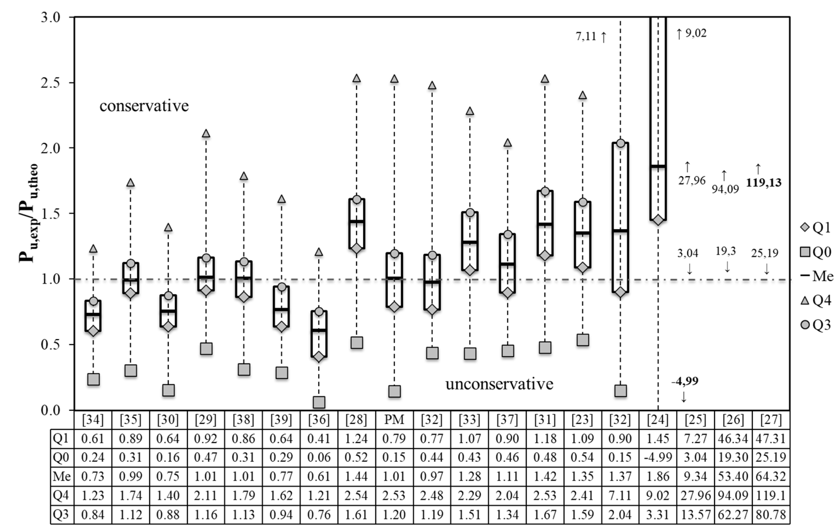
| Quartile | Value |
|---|---|
| Q0 | 0.15 |
| Q1 | 0.79 |
| Q3 | 1.20 |
| Q4 | 2.53 |
| Me | 1.01 |
| References | Year | IQR | K | as1 | as2 | as3 |
|---|---|---|---|---|---|---|
| [34] | 2005 | 0.23 | 2.88 | 0.00 | 0.00 | −0.11 |
| [35] | 2005 | 0.23 | 3.75 | 0.00 | 0.00 | 0.25 |
| [30] | 2001 | 0.24 | 3.28 | 0.00 | 0.00 | 0.09 |
| [29] | 2001 | 0.25 | 4.49 | 0.50 | 1.50 | 0.50 |
| [38] | 2012 | 0.27 | 3.24 | 0.50 | 1.50 | 0.08 |
| [39] | 2013 | 0.30 | 3.09 | 0.00 | 0.00 | 0.34 |
| [36] | 2009 | 0.35 | 2.45 | −0.50 | −1.50 | −0.25 |
| [28] | 2000 | 0.38 | 3.17 | 0.50 | 1.50 | 0.11 |
| Proposed Model [[–] | - | 0.41 | 4.86 | 0.00 | 0.00 | 0.00 |
| [32] | 2003 | 0.42 | 4.69 | −0.50 | −1.50 | 0.11 |
| [33] | 2004 | 0.44 | 2.64 | 0.00 | 0.00 | 0.01 |
| [37] | 2010 | 0.45 | 4.02 | 0.00 | 0.00 | 0.72 |
| [31] | 2001 | 0.45 | 2.70 | 0.50 | 1.50 | 0.24 |
| [23] | 1994 | 0.49 | 2.64 | 0.00 | 0.00 | 0.01 |
| [22] | 1980 | 1.14 | 7.76 | 0.50 | 1.50 | 0.52 |
| [24] | 1996 | 1.85 | 7.43 | 0.50 | 1.50 | 1.02 |
| [25] | 1997 | 6.29 | 3.55 | 0.50 | 1.50 | 0.90 |
| [26] | 1997 | 15.92 | 3.16 | 0.00 | 0.00 | 0.36 |
| [27] | 1998 | 33.46 | 2.17 | −0.50 | −1.50 | 0.09 |
| Max | 33.46 | 7.76 | 0.50 | 1.50 | 1.02 | |
| Min | 0.23 | 2.17 | 0.00 | 0.00 | 0.00 | |
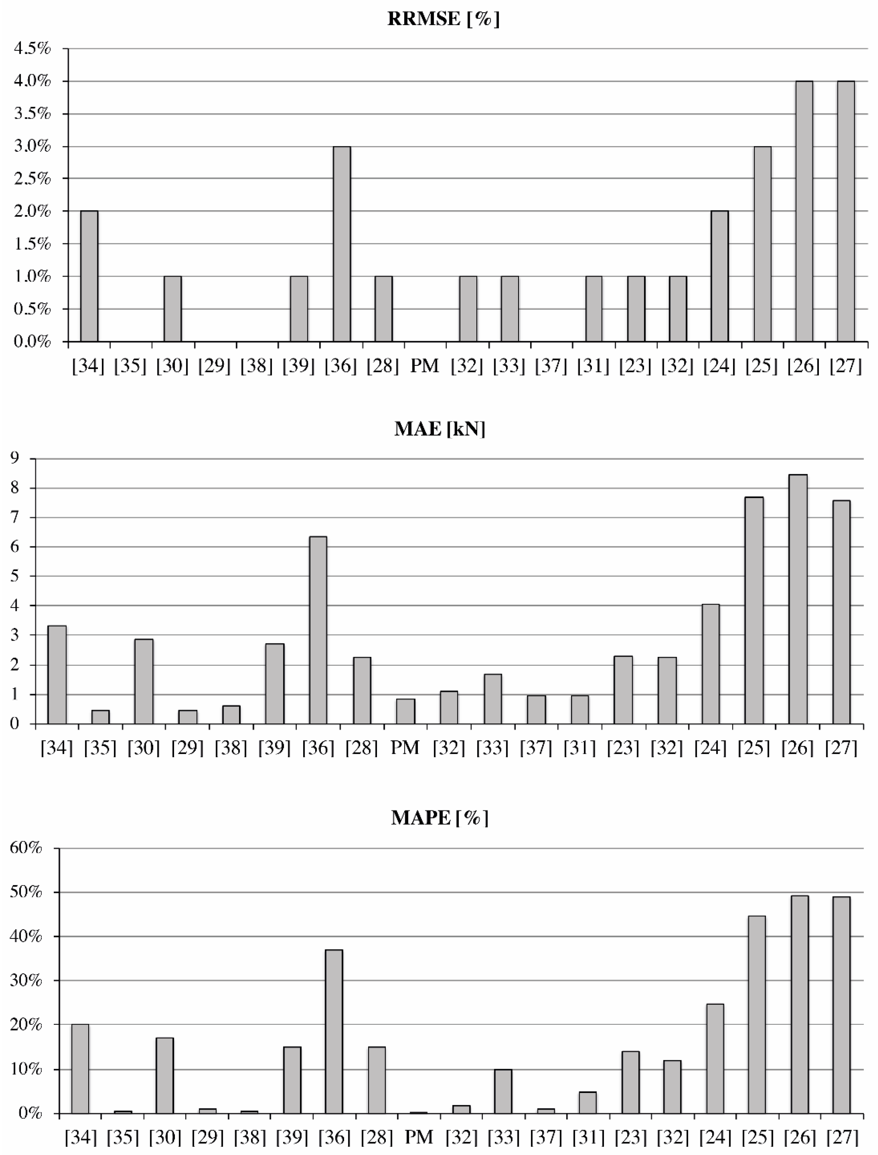
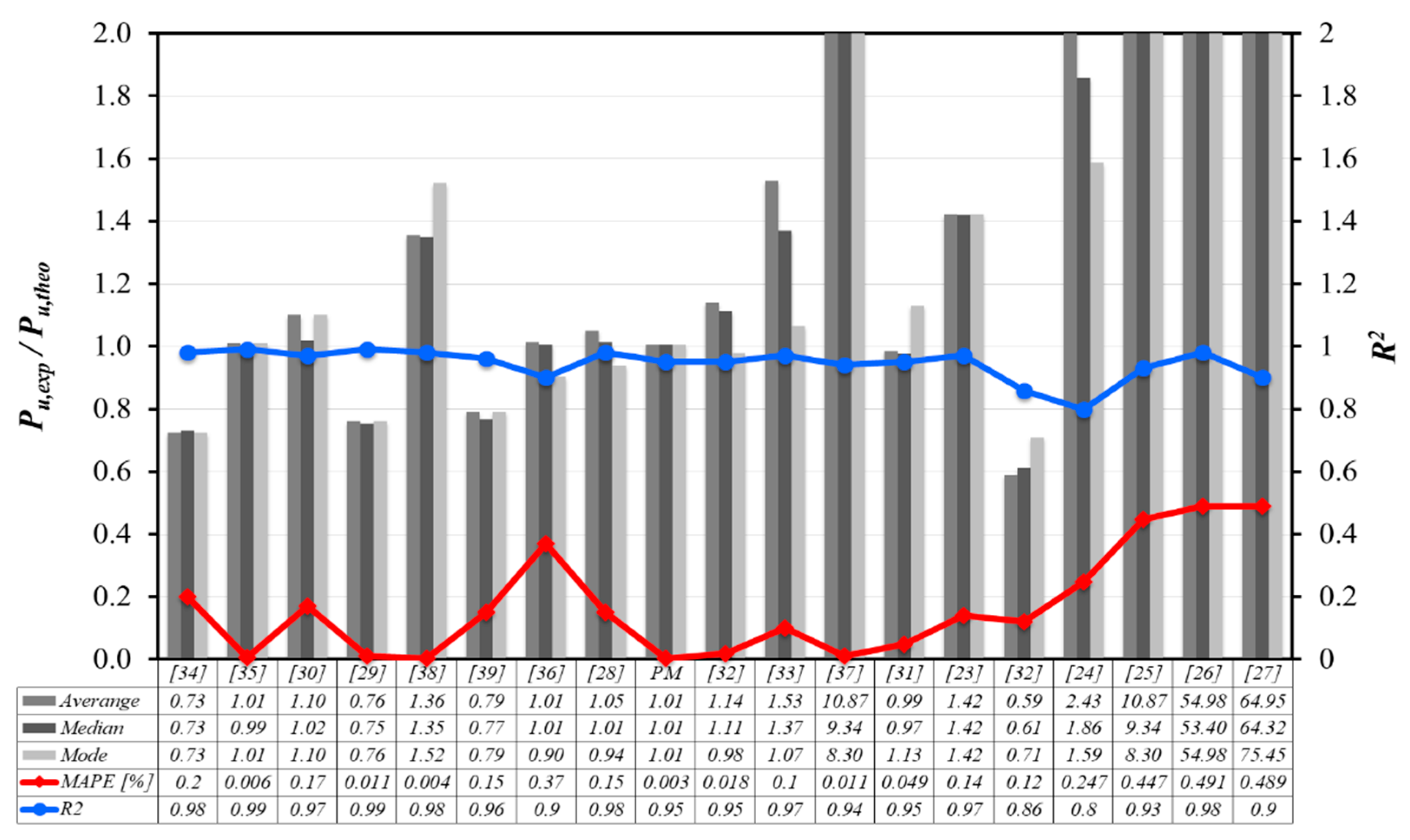
| References | RRMSE (%) | MAE (kN) | MAPE (%) | R2 |
|---|---|---|---|---|
| [34] | 2.00% | 3.34 | 20.00% | 0.98 |
| [35] | 0.00% | 0.46 | 0.60% | 0.99 |
| [30] | 1.00% | 2.87 | 17.00% | 0.97 |
| [29] | 0.00% | 0.46 | 1.10% | 0.99 |
| [38] | 0.00% | 0.61 | 0.40% | 0.98 |
| [39] | 1.00% | 2.71 | 15.00% | 0.96 |
| [36] | 3.00% | 6.35 | 37.00% | 0.90 |
| [28] | 1.00% | 2.26 | 15.00% | 0.98 |
| Proposed Model [–] | 0.00% | 0.84 | 0.30% | 0.95 |
| [32] | 1.00% | 1.09 | 1.80% | 0.95 |
| [33] | 1.00% | 1.67 | 10.00% | 0.97 |
| [37] | 0.00% | 0.95 | 1.10% | 0.94 |
| [31] | 1.00% | 0.96 | 4.90% | 0.95 |
| [23] | 1.00% | 2.29 | 14.00% | 0.97 |
| [22] | 1.00% | 2.27 | 12.00% | 0.86 |
| [24] | 2.00% | 4.05 | 24.70% | 0.80 |
| [25] | 3.00% | 7.69 | 44.70% | 0.93 |
| [26] | 4.00% | 8.43 | 49.10% | 0.98 |
| [27] | 4.00% | 7.56 | 48.90% | 0.90 |
| Max | 4.00% | 8.43 | 49.10 | 0.99 |
| Min | 0.00 | 0.46 | 0.30% | 0.80 |
Publisher’s Note: MDPI stays neutral with regard to jurisdictional claims in published maps and institutional affiliations. |
© 2021 by the authors. Licensee MDPI, Basel, Switzerland. This article is an open access article distributed under the terms and conditions of the Creative Commons Attribution (CC BY) license (https://creativecommons.org/licenses/by/4.0/).
Share and Cite
Cascardi, A.; Micelli, F. ANN-Based Model for the Prediction of the Bond Strength between FRP and Concrete. Fibers 2021, 9, 46. https://doi.org/10.3390/fib9070046
Cascardi A, Micelli F. ANN-Based Model for the Prediction of the Bond Strength between FRP and Concrete. Fibers. 2021; 9(7):46. https://doi.org/10.3390/fib9070046
Chicago/Turabian StyleCascardi, Alessio, and Francesco Micelli. 2021. "ANN-Based Model for the Prediction of the Bond Strength between FRP and Concrete" Fibers 9, no. 7: 46. https://doi.org/10.3390/fib9070046