Triple Local Similarity Solutions of Darcy-Forchheimer Magnetohydrodynamic (MHD) Flow of Micropolar Nanofluid Over an Exponential Shrinking Surface: Stability Analysis

 ,
,  and
and 
Abstract
:1. Introduction
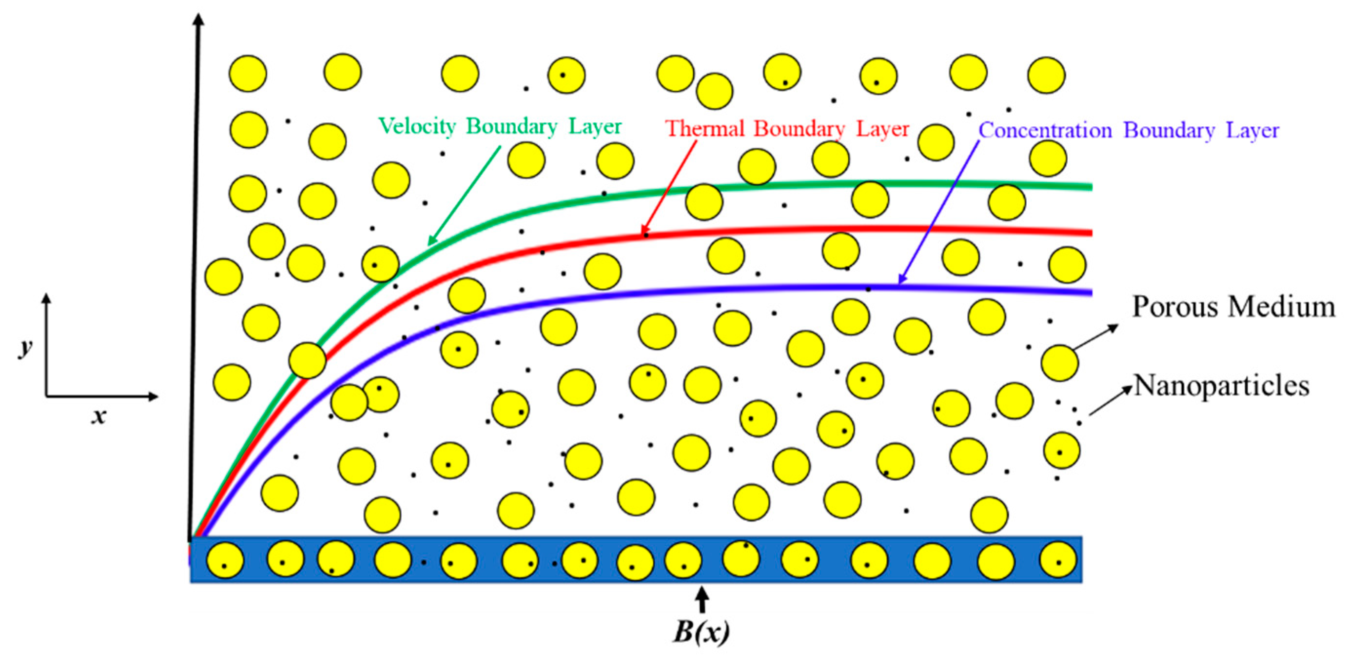
2. Problem Description and Formulation
3. Stability Analysis
4. Results and Discussion
5. Conclusions
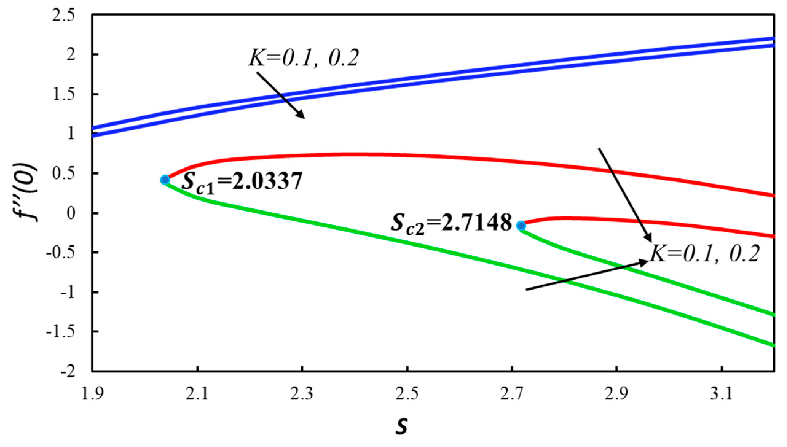
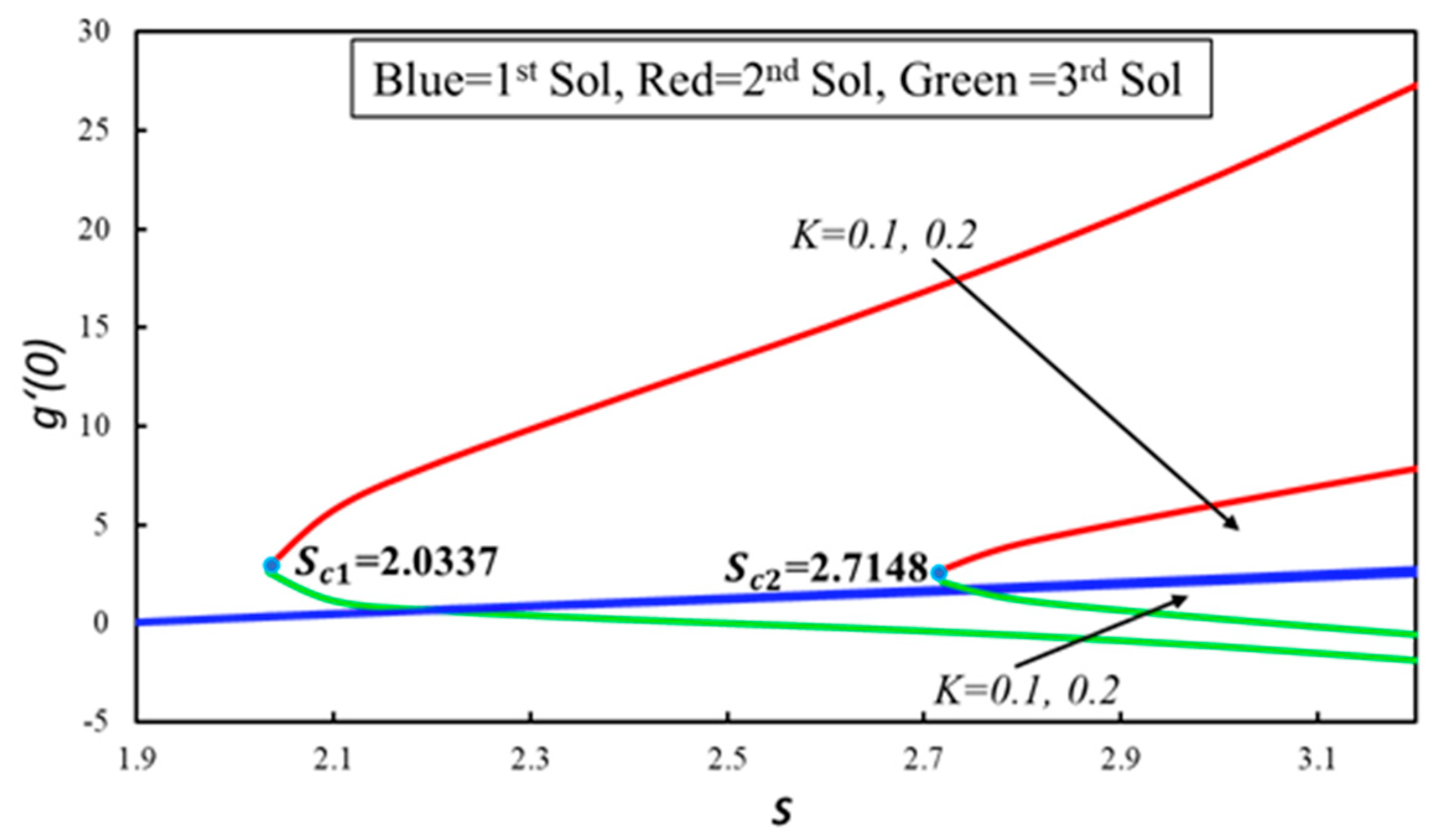
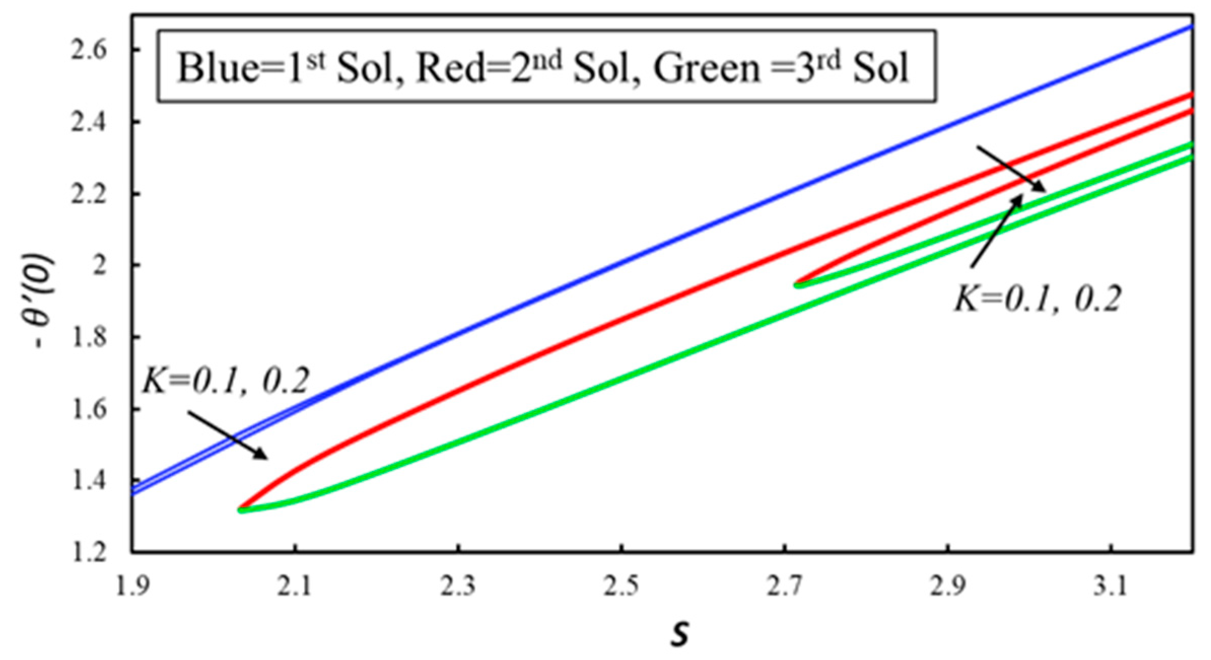
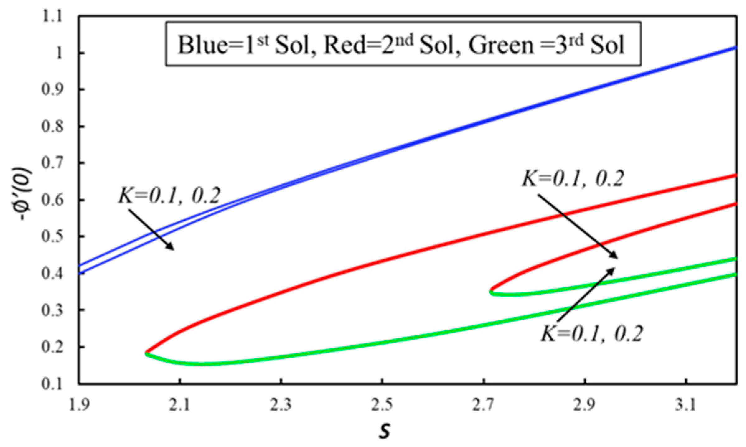
- Triple solutions exist when for and when for .
- Dual solutions exist for the Newtonian case .
- The study of critical points acknowledges the range of multiple solutions and single solutions.
- The study of the stability analysis indicates that only the first solution is stable and that the remaining two solutions are unstable.
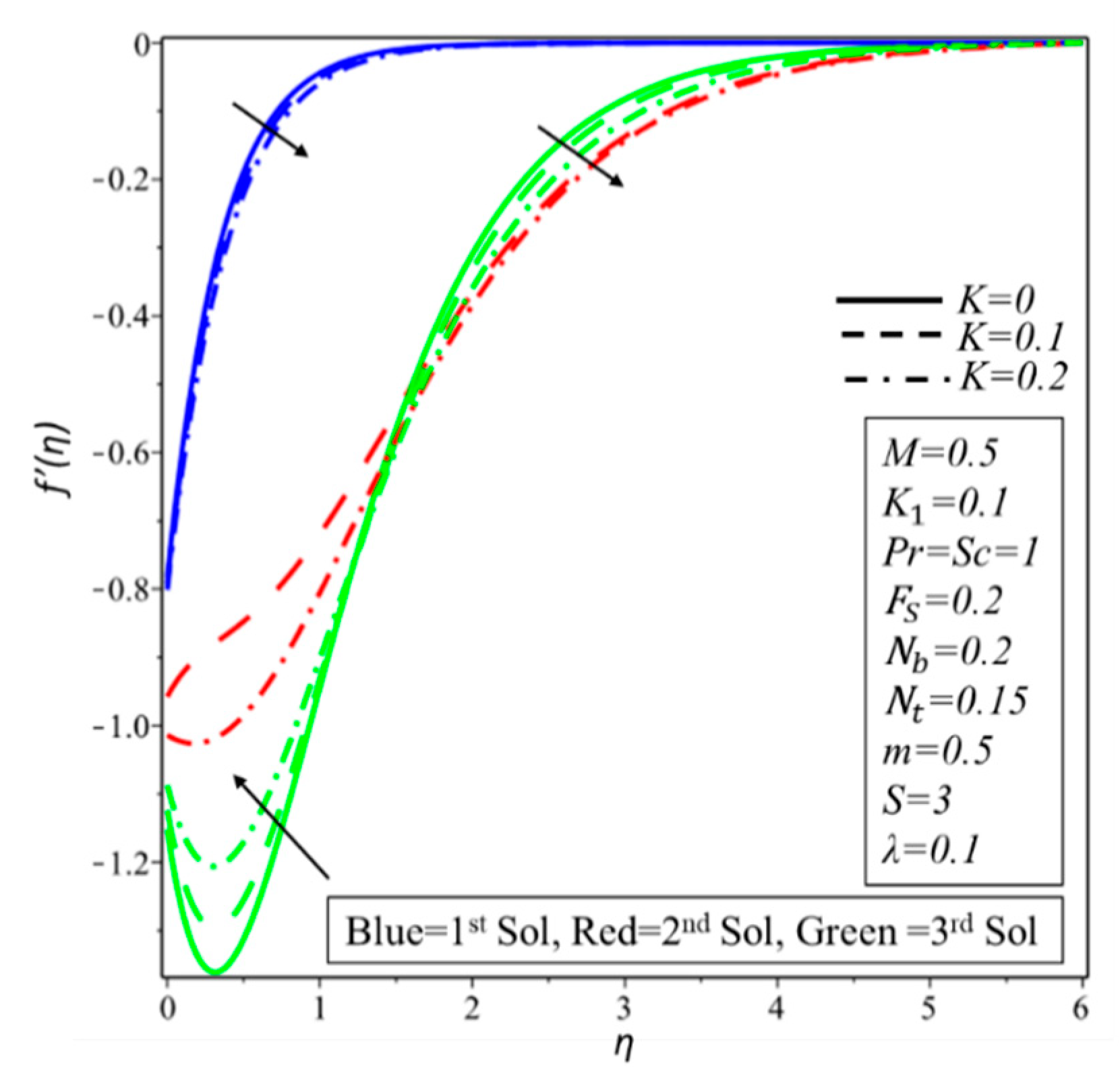
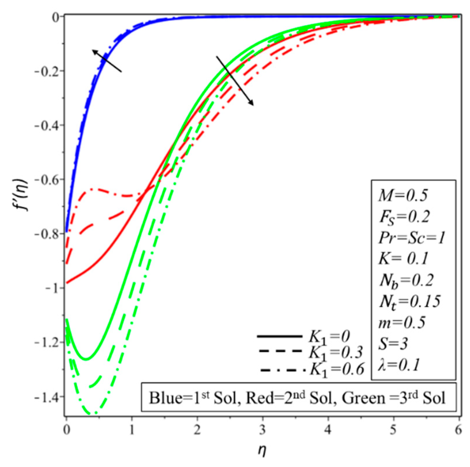
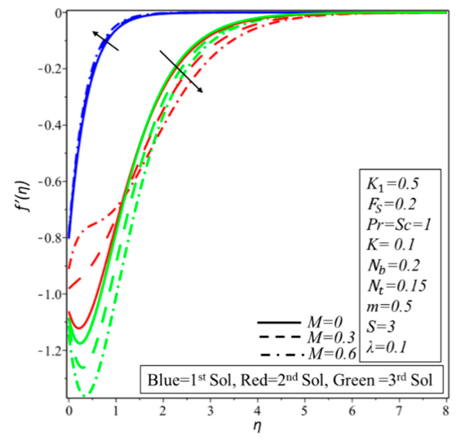
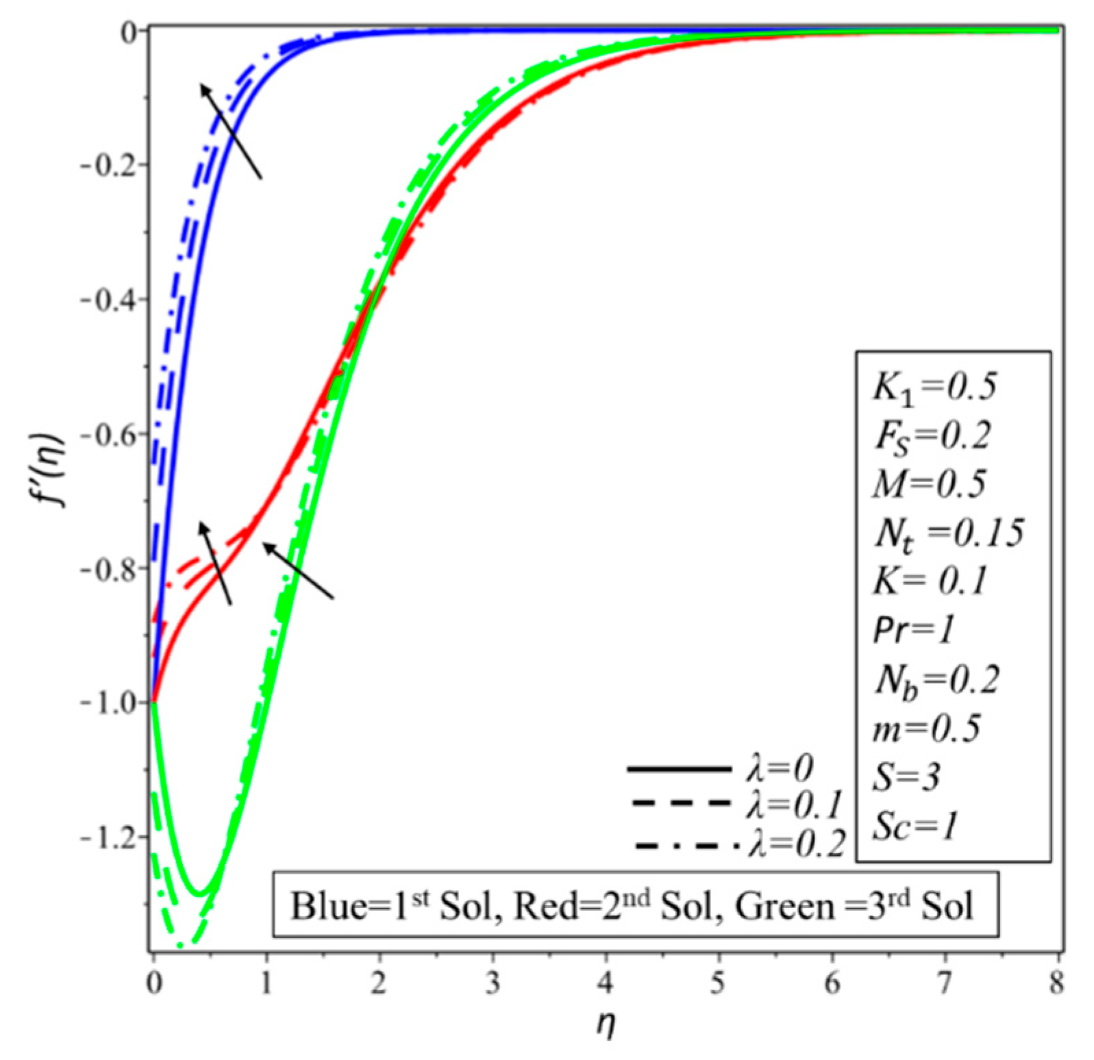
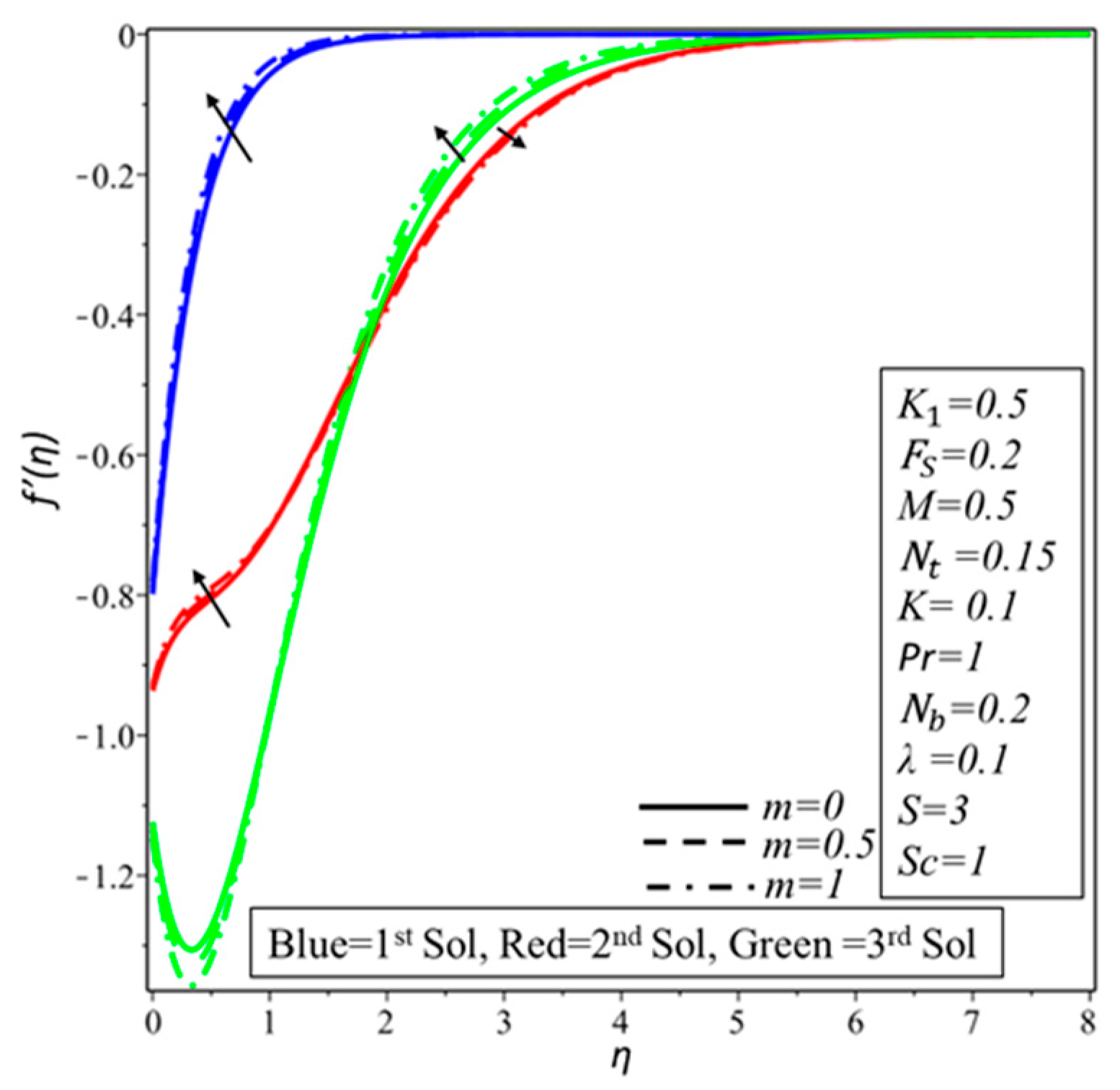
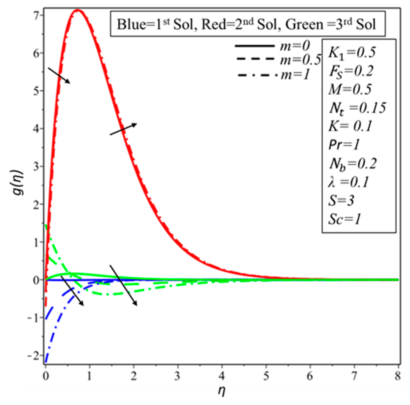
- The thickness of the momentum boundary layer decreases with increasing values of and in the first solution.
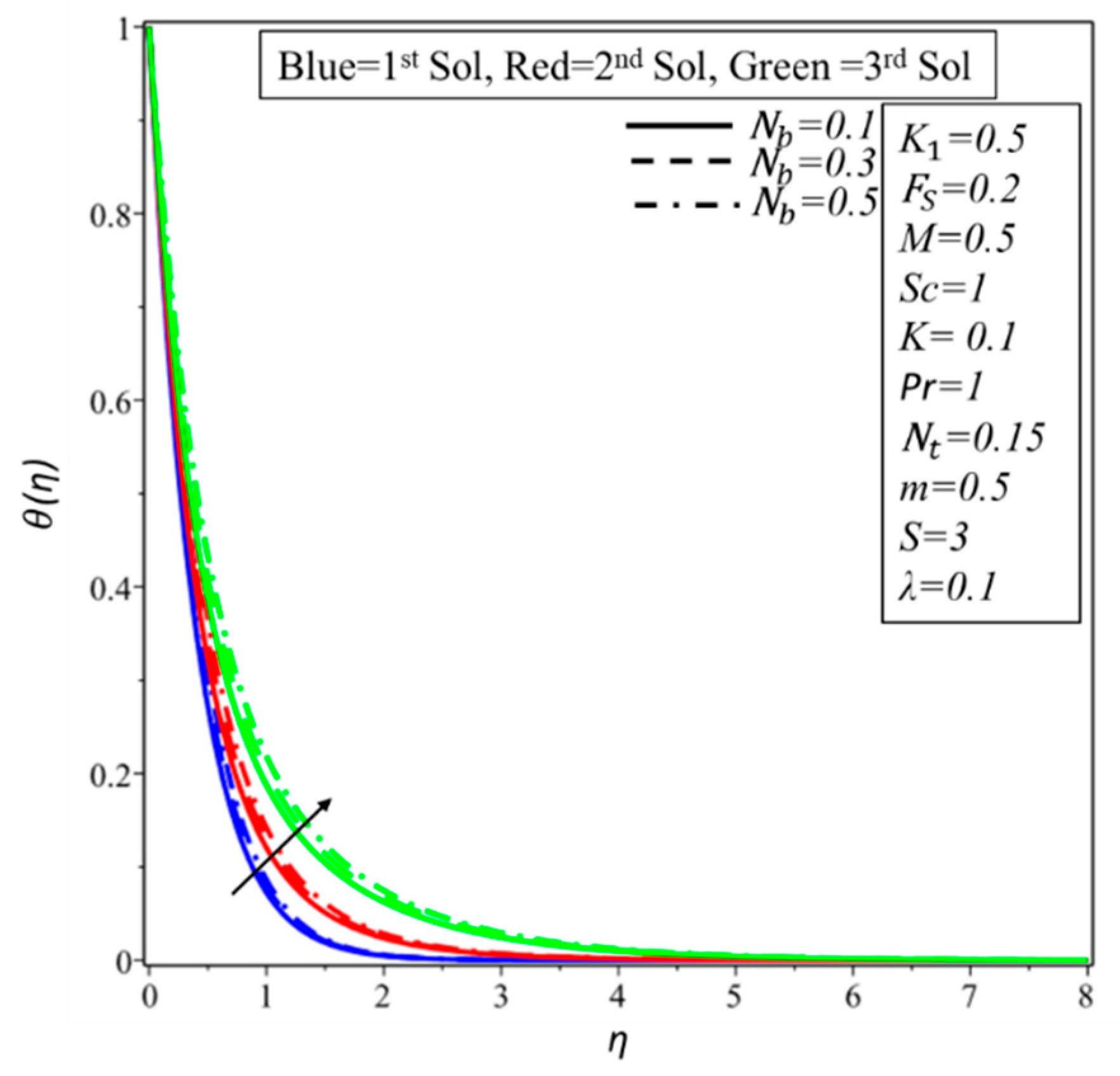
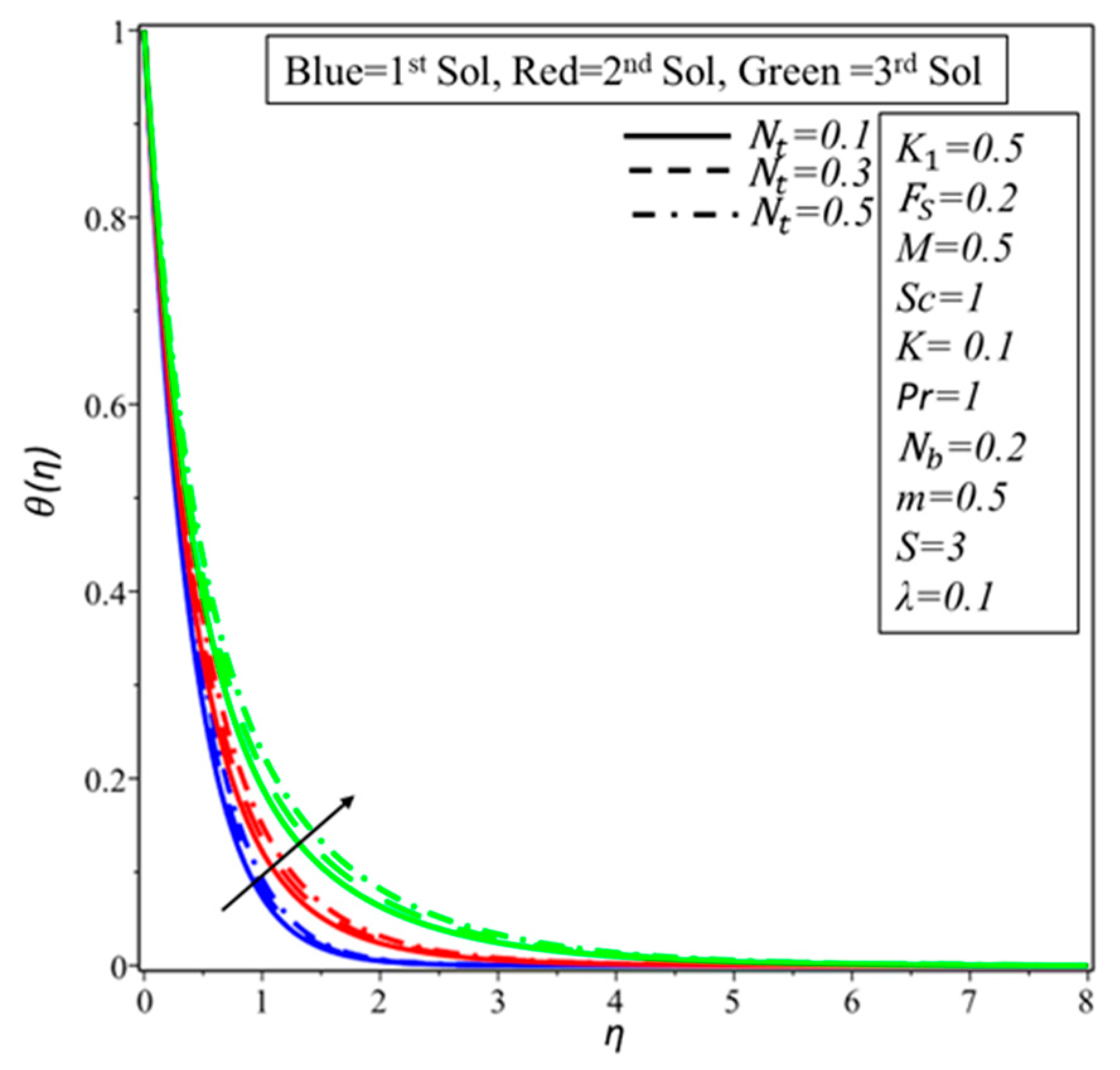
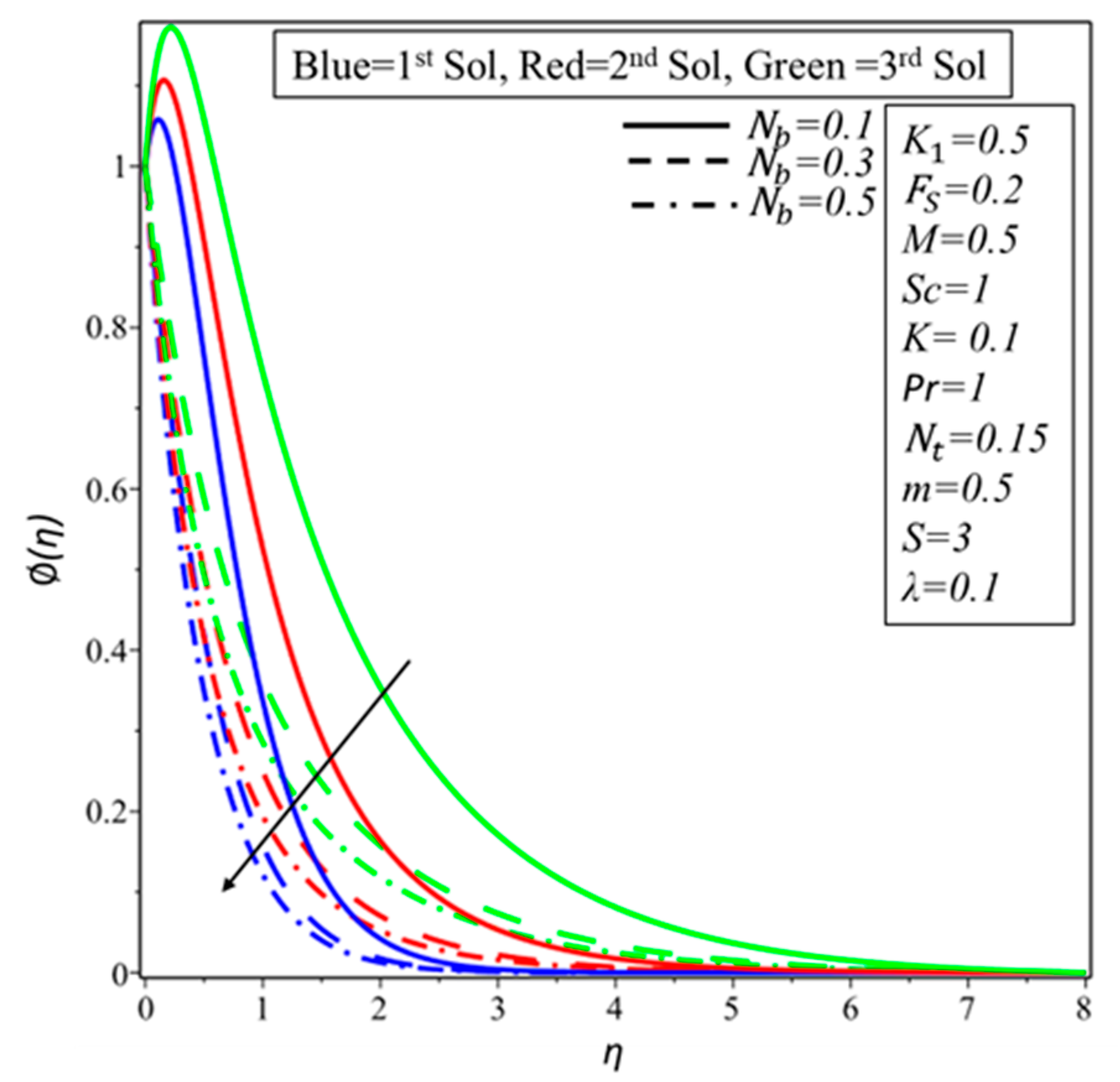
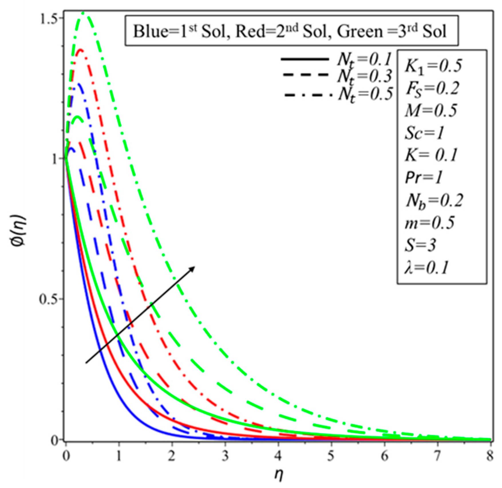
- Increasing values of thermophoresis and Brownian motion parameters are caused by the thickness of the thermal boundary layer.
Author Contributions
Funding
Acknowledgments
Conflicts of Interest
Nomenclature
| u, v | velocity components |
| surface velocity | |
| N | microrotation |
| K | material parameter |
| M | a constant |
| T | temperature |
| a constant | |
| variable temperature at the sheet | |
| ambient temperature | |
| C | concentration |
| a constant | |
| ambient concentration | |
| kinematic viscosity | |
| vortex viscosity | |
| spin gradient viscosity | |
| microinertia per unit mass | |
| thermal diffusivity | |
| thermal conductivity | |
| stream function | |
| transformed variable | |
| B(x) | magnetic field |
| b | local inertia coefficient |
| M | Hartmann number |
| Pr | Prandtl number |
| Brownian diffusion | |
| thermophoretic diffusion | |
| suction/injection velocity | |
| permeability of the porous medium | |
| variable concentration at the sheet | |
| thermophoresis parameter | |
| Schmidt number | |
| Velocity slip | |
| S | injunction/suction parameter |
| skin friction coefficient | |
| local Nusselt number | |
| Brownian motion parameter | |
| local Sherwood number | |
| local Reynolds number | |
| unknown eigen value | |
| Stability transformed variable |
References
- Dero, S.; Rohni, A.M.; Saaban, A. MHD micropolar nanofluid flow over an exponentially stretching/shrinking surface: Triple solutions. J. Adv. Res. Fluid Mech. Therm. Sci. 2019, 56, 165–174. [Google Scholar]
- Ariman, T.T.N.D.; Turk, M.A.; Sylvester, N.D. Microcontinuum fluid mechanics—A review. Int. J. Eng. Sci. 1973, 11, 905–930. [Google Scholar] [CrossRef]
- Ariman, T.T.N.D.; Turk, M.A.; Sylvester, N.D. Applications of microcontinuum fluid mechanics. Int. J. Eng. Sci. 1974, 12, 273–293. [Google Scholar] [CrossRef]
- Eringen, A.C. Theory of micropolar fluids. J. Math. Mech. 1966, 16, 1–18. [Google Scholar] [CrossRef]
- Eringen, A.C. Theory of thermomicrofluids. J. Math. Anal. Appl. 1972, 38, 480–496. [Google Scholar] [CrossRef] [Green Version]
- Eringen, A.C. Microcontinuum Field Theories: I. Foundations and Solids; Springer: Heidelberg, Germany, 2012. [Google Scholar]
- Lukaszewicz, G. Micropolar Fluids: Theory and Applications; Springer: Cambridge, MA, USA, 1999. [Google Scholar]
- Kumar, G.C.; Reddy, K.J.; Konijeti, R.K.; Reddy, M.N. Non-uniform heat source/sink and joule heating effects on chemically radiative MHD mixed convective flow of micropolar fluid over a stretching sheet in porous medium. Defect Diffus. Forum 2018, 388, 281–302. [Google Scholar] [CrossRef]
- Gupta, D.; Kumar, L.; Bég, O.A.; Singh, B. Finite element analysis of MHD flow of micropolar fluid over a shrinking sheet with a convective surface boundary condition. J. Eng. Thermophys. 2018, 27, 202–220. [Google Scholar] [CrossRef]
- Turkyilmazoglu, M. Mixed convection flow of magnetohydrodynamic micropolar fluid due to a porous heated/cooled deformable plate: Exact solutions. Int. J. Heat Mass Transf. 2017, 106, 127–134. [Google Scholar] [CrossRef]
- Sheikh, N.A.; Ali, F.; Khan, I.; Saqib, M.; Khan, A. MHD flow of micropolar fluid over an oscillating vertical plate embedded in porous media with constant temperature and concentration. Math. Probl. Eng. 2017, 2017, 9402964. [Google Scholar] [CrossRef]
- Akhter, S.; Ashraf, M.; Ali, K. MHD flow and heat transfer analysis of micropolar fluid through a porous medium between two stretchable disks using quasi-linearization method. Iran. J. Chem. Chem. Eng. 2017, 36, 155–169. [Google Scholar]
- Siddiq, M.; Rauf, A.; Shehzad, S.; Abbasi, F.; Meraj, M. Thermally and solutally convective radiation in mhd stagnation point flow of micropolar nanofluid over a shrinking sheet. Alex. Eng. J. 2018, 57, 963–971. [Google Scholar] [CrossRef]
- Dero, S.; Uddin, M.J.; Rohni, A.M. Stefan blowing and slip effects on unsteady nanofluid transport past a shrinking sheet: Multiple solutions. Heat Transf. Asian Res. 2019. [Google Scholar] [CrossRef]
- Hayat, T.; Sajjad, R.; Ellahi, R.; Alsaedi, A.; Muhammad, T. Homogeneous-heterogeneous reactions in MHD flow of micropolar fluid by a curved stretching surface. J. Mol. Liq. 2017, 240, 209–220. [Google Scholar] [CrossRef]
- Hayat, T.; Saif, R.S.; Ellahi, R.; Muhammad, T.; Ahmad, B. Numerical study for darcy-forchheimer flow due to a curved stretching surface with cattaneo-christov heat flux and homogeneous-heterogeneous reactions. Results Phys. 2017, 7, 2886–2892. [Google Scholar] [CrossRef]
- Ahmed, B.; Javed, T.; Ali, N. Numerical study at moderate Reynolds number of peristaltic flow of micropolar fluid through a porous-saturated channel in magnetic field. AIP Adv. 2018, 8, 015319. [Google Scholar] [CrossRef] [Green Version]
- Waqas, M.; Farooq, M.; Khan, M.I.; Alsaedi, A.; Hayat, T.; Yasmeen, T. Magnetohydrodynamic (MHD) mixed convection flow of micropolar liquid due to nonlinear stretched sheet with convective condition. Int. J. Heat Mass Transf. 2016, 102, 766–772. [Google Scholar] [CrossRef]
- Das, S.K.; Choi, S.U.; Yu, W.; Pradeep, T. Nanofluids: Science and Technology; John Wiley & Sons: Hoboken, NJ, USA, 2007. [Google Scholar]
- Dero, S.; Rohni, A.M.; Saaban, A. The dual solutions and stability analysis of nanofluid flow using tiwari-das modelover a permeable exponentially shrinking surface with partial slip conditions. J. Eng. Appl. Sci. 2019, 14, 4569–4582. [Google Scholar] [CrossRef]
- Choi, S.U.; Eastman, J.A. Enhancing thermal conductivity of fluids with nanoparticles. ASME Publ. Fed 1995, 231, 99–106. [Google Scholar]
- Oztop, H.F.; Abu-Nada, E. Numerical study of natural convection in partially heated rectangular enclosures filled with nanofluids. Int. J. Heat Fluid Flow 2008, 29, 1326–1336. [Google Scholar] [CrossRef]
- Khanafer, K.; Vafai, K.; Lightstone, M. Buoyancy-driven heat transfer enhancement in a two-dimensional enclosure utilizing nanofluids. Int. J. Heat Mass Transf. 2003, 46, 3639–3653. [Google Scholar] [CrossRef]
- Buongiorno, J. Convective transport in nanofluids. J. Heat Transf. 2006, 128, 240–250. [Google Scholar] [CrossRef]
- Nield, D.A.; Bejan, A. Convection in Porous Media; Springer: New York, NY, USA, 2006. [Google Scholar]
- Mahian, O.; Kolsi, L.; Amani, M.; Estellé, P.; Ahmadi, G.; Kleinstreuer, C.; Marshall, J.S.; Siavashi, M.; Taylor, R.A.; Niazmand, H. Recent advances in modeling and simulation of nanofluid flows-part I: Fundamental and theory. Phys. Rep. 2019, 790, 1–48. [Google Scholar] [CrossRef]
- Mahian, O.; Kolsi, L.; Amani, M.; Estellé, P.; Ahmadi, G.; Kleinstreuer, C.; Marshall, J.S.; Taylor, R.A.; Abu-Nada, E.; Rashidi, S. Recent advances in modeling and simulation of nanofluid flows-part II: Applications. Phys. Rep. 2019, 791, 1–59. [Google Scholar] [CrossRef]
- Mahian, O.; Kianifar, A.; Kalogirou, S.A.; Pop, I.; Wongwises, S. A review of the applications of nanofluids in solar energy. Int. J. Heat Mass Transf. 2013, 57, 582–594. [Google Scholar] [CrossRef]
- Wong, K.V.; De Leon, O. Applications of nanofluids: Current and future. Adv. Mech. Eng. 2010, 2, 519659. [Google Scholar] [CrossRef]
- Mahdy, A. Simultaneous impacts of mhd and variable wall temperature on transient mixed casson nanofluid flow in the stagnation point of rotating sphere. Appl. Math. Mech. 2018, 39, 1327–1340. [Google Scholar] [CrossRef]
- Rehman, K.U.; Malik, M.; Zahri, M.; Tahir, M. Numerical analysis of MHD casson navier’s slip nanofluid flow yield by rigid rotating disk. Results Phys. 2018, 8, 744–751. [Google Scholar] [CrossRef]
- Hamid, M.; Usman, M.; Khan, Z.; Haq, R.; Wang, W. Numerical study of unsteady MHD flow of williamson nanofluid in a permeable channel with heat source/sink and thermal radiation. Eur. Phys. J. Plus 2018, 133, 527. [Google Scholar] [CrossRef]
- Eid, M.R.; Mahny, K.L.; Muhammad, T.; Sheikholeslami, M. Numerical treatment for carreau nanofluid flow over a porous nonlinear stretching surface. Results Phys. 2018, 8, 1185–1193. [Google Scholar] [CrossRef]
- Prabhakar, B.; Bandari, S.; Reddy, C.S. A revised model to analyze MHD flow of maxwell nanofluid past a stretching sheet with nonlinear thermal radiation effect. Int. J. Fluid Mech. Res. 2019, 46, 151–165. [Google Scholar] [CrossRef]
- Guedda, M.; Hammouch, Z. On similarity and pseudo-similarity solutions of falkner–skan boundary layers. Fluid Dyn. Res. 2006, 38, 211–223. [Google Scholar] [CrossRef]
- Minkowycz, W.; Sparrow, E. Local nonsimilar solutions for natural convection on a vertical cylinder. J. Heat Transf. 1974, 96, 178–183. [Google Scholar] [CrossRef]
- Ming-Jer, H.; Cha’o-Kuang, C. Local similarity solutions of free convective heat transfer from a vertical plate to non-newtonian power law fluids. Int. J. Heat Mass Transf. 1990, 33, 119–125. [Google Scholar] [CrossRef]
- Zhang, Z. Normal solutions of a boundary-value problem arising in free convection boundary-layer flows in porous media. Appl. Math. Comput. 2018, 339, 367–373. [Google Scholar] [CrossRef]
- Sanjayanand, E.; Khan, S.K. On heat and mass transfer in a viscoelastic boundary layer flow over an exponentially stretching sheet. Int. J. Therm. Sci. 2006, 45, 819–828. [Google Scholar] [CrossRef]
- Jena, S.K.; Mathur, M. Similarity solutions for laminar free convection flow of a thermomicropolar fluid past a non-isothermal vertical flat plate. Int. J. Eng. Sci. 1981, 19, 1431–1439. [Google Scholar] [CrossRef]
- Ishak, A.; Nazar, R.; Pop, I. Heat transfer over a stretching surface with variable heat flux in micropolar fluids. Phys. Lett. A 2008, 372, 559–561. [Google Scholar] [CrossRef]
- Weidman, P.; Kubitschek, D.; Davis, A. The effect of transpiration on self-similar boundary layer flow over moving surfaces. Int. J. Eng. Sci. 2006, 44, 730–737. [Google Scholar] [CrossRef]
- Roşca, A.V.; Pop, I. Flow and heat transfer over a vertical permeable stretching/shrinking sheet with a second order slip. Int. J. Heat Mass Transf. 2013, 60, 355–364. [Google Scholar] [CrossRef]
- Ali Lund, L.; Omar, Z.; Khan, I.; Raza, J.; Bakouri, M.; Tlili, I. Stability analysis of darcy-forchheimer flow of casson type nanofluid over an exponential sheet: Investigation of critical points. Symmetry 2019, 11, 412. [Google Scholar] [CrossRef]
- Lund, L.A.; Omar, Z.; Khan, I. Analysis of dual solution for MHD flow of Williamson fluid with slippage. Heliyon 2019, 5, e01345. [Google Scholar] [CrossRef] [Green Version]
- Rahman, M.; Rosca, A.V.; Pop, I. Boundary layer flow of a nanofluid past a permeable exponentially shrinking surface with convective boundary condition using buongiorno’s model. Int. J. Numer. Methods Heat Fluid Flow 2015, 25, 299–319. [Google Scholar] [CrossRef]
- Alarifi, I.M.; Abokhalil, A.G.; Osman, M.; Lund, L.A.; Ayed, M.B.; Belmabrouk, H.; Tlili, I. MHD flow and heat transfer over vertical stretching sheet with heat sink or source effect. Symmetry 2019, 11, 297. [Google Scholar] [CrossRef]
- Harris, S.D.; Ingham, D.B.; Pop, I. Mixed convection boundary-layer flow near the stagnation point on a vertical surface in a porous medium: Brinkman model with slip. Transp. Porous Media 2009, 77, 267–285. [Google Scholar] [CrossRef]
- Wang, C. Liquid film on an unsteady stretching surface. Q. Appl. Math. 1990, 48, 601–610. [Google Scholar] [CrossRef] [Green Version]


| 1st Solution | 2nd Solution | 3rd Solution | ||
|---|---|---|---|---|
| 0.1 | 2.5 | 1.4309 | −1.2683 | −0.9436 |
| 3 | 1.7854 | −1.3162 | −1.2053 | |
| 0.2 | 3 | 0.9831 | −0.4392 | −0.3518 |
| 3.5 | 1.2165 | −0.6431 | −0.5382 | |
© 2019 by the authors. Licensee MDPI, Basel, Switzerland. This article is an open access article distributed under the terms and conditions of the Creative Commons Attribution (CC BY) license (http://creativecommons.org/licenses/by/4.0/).
Share and Cite
Ali Lund, L.; Ching, D.L.C.; Omar, Z.; Khan, I.; Nisar, K.S. Triple Local Similarity Solutions of Darcy-Forchheimer Magnetohydrodynamic (MHD) Flow of Micropolar Nanofluid Over an Exponential Shrinking Surface: Stability Analysis. Coatings 2019, 9, 527. https://doi.org/10.3390/coatings9080527
Ali Lund L, Ching DLC, Omar Z, Khan I, Nisar KS. Triple Local Similarity Solutions of Darcy-Forchheimer Magnetohydrodynamic (MHD) Flow of Micropolar Nanofluid Over an Exponential Shrinking Surface: Stability Analysis. Coatings. 2019; 9(8):527. https://doi.org/10.3390/coatings9080527
Chicago/Turabian StyleAli Lund, Liaquat, Dennis Ling Chuan Ching, Zurni Omar, Ilyas Khan, and Kottakkaran Sooppy Nisar. 2019. "Triple Local Similarity Solutions of Darcy-Forchheimer Magnetohydrodynamic (MHD) Flow of Micropolar Nanofluid Over an Exponential Shrinking Surface: Stability Analysis" Coatings 9, no. 8: 527. https://doi.org/10.3390/coatings9080527