Incorporating Physics-Based Models into Equivalent Circuit Analysis of EIS Data from Organic Coatings

Abstract

Electrochemical impedance spectroscopy (EIS) is a widely used method for monitoring coatings because it can be done in situ and causes little damage to the coating. However, interpreting the impedance data from coatings in order to determine the state of the coating and its protective abilities is challenging. A modified version of the rapid electrochemical assessment of paint (REAP) equivalent circuit is developed here, along with a method to calculate the impedance of a circuit using matrix algebra. This new equivalent circuit and the calculation method are used to analyze EIS data obtained from a two-layer commercial organic coating system immersed in NaCl solutions with different concentrations and at different temperatures. The matrix calculation method is validated by comparing results obtained from commercial analysis software to this method for two different equivalent circuits, and the parameter values are nearly equal. Physics-based models of the equivalent circuit elements are derived and used to obtain both initial estimates for the regressions and physics-based constraints on the model parameters. These models are integrated into the regression procedure, and the corrected Akaike information criterion (AICc) is used to compare fits between the new circuit and classic equivalent circuits. The AICc values indicate the new circuit results in better fits than classic equivalent circuits used for coatings analysis.

1. Introduction

Organic polymer coatings are commonly used to protect metal aircraft structures from corrosion. This protection can be broadly classified into three categories: a cross-linked network that provides a barrier against the ingress of electrolyte ions, such as chloride (Cl⁻) [1], active inhibition via a reservoir of inorganic or organometallic inhibitors, and surface hydrophobicity. While the protective characteristics of the first two categories benefit from the application of thicker coatings, the need to minimize the weight added to an aircraft constrains the overall coating thickness.

Environmental exposure of aircraft-grade polymeric coatings to ultraviolet radiation from sunlight and seawater results in coating deterioration, which is observed as a reduction in chemical cross-links and subsequent loss of mechanical properties [2]. This deterioration is characterized by a sequential progression of behaviors, including: diffusion of water and dissolved oxygen; transport of electrolyte ions; development of anodic and cathodic regions at the coating-substrate interface; onset of electrochemical reactions; chemical and hydrolysis reactions; displacement of polymer-surface bonds by water-surface bonds and accumulation of water to form blisters [3] or the formation corrosion products at the coating-oxide interface, both of which result in loss of coating-to-surface adhesion [4,5]. Because of this deterioration progression, for many commercial and military aircraft, coating system removal for inspections and mitigation actions are planned prior to the onset of corrosion damage. As the state of the coating and the underlying substrate are usually not known, these removal and repainting operations are performed on a time-based, rather than condition-based schedule. These processes generate large quantities of waste that must be properly handled and can expose workers to toxic materials [6]. Thus, from a maintenance and environmental perspective, there is much interest in reducing the number of aircraft paint removal coating operations to the minimum necessary, preferably basing these decisions on the condition of the coating.

Because coating deterioration in the early stages can be difficult to ascertain visually, other evaluation methods are used. One frequently employed technique is electrochemical impedance spectroscopy (EIS) [7]. EIS is a useful technique for monitoring coatings because the measurements can be made with little disruption [8]. However, EIS data provides only indirect evidence of the state of an organic coating system, and one of the challenges with using EIS data is assigning the correct physical interpretation to the impedance. Analyses are usually performed using equivalent circuit models with the circuit element parameter values providing insight into the state of the coating.

EIS data analysis for organic coatings has traditionally focused on determining coating resistance or capacitance as a means of assessing the state of the coating. Lee and Mansfeld [9] suggested classifying coatings as good, intermediate, or bad if the pore resistance of the coating ranged 50–500 $\mathrm{G}\Omega ·\mathrm{c}{\mathrm{m}}^2$, 50–500 $\mathrm{M}\Omega ·\mathrm{c}{\mathrm{m}}^2$, or 0.1–5 $\mathrm{M}\Omega ·\mathrm{c}{\mathrm{m}}^2$, respectively. They based this classification on three-layer coating systems of various types applied to steel coupons and immersed in seawater for up to two years [10,11]. This approach for characterizing the state of a coating system is the most widely used.

However, for commercial aircraft coating systems, like the one studied in this work, the impedance response is dominated by the coating capacitance during most of its life cycle [12]. Water uptake by the polymer that forms the coating binder changes the dielectric properties of the coating because the dielectric constant of the polymer-water-air system is assumed to correspond to some ratio of the values, as seen in (1) [13],

$${ϵ}_i={ϵ}_p^{\frac{V_p}{V}}{ϵ}_{H_{2}O}^{\frac{V_{H_{2}O}}{V}}{ϵ}_0^{\frac{V_0}{V}},$$

(1)

where ${ϵ}_i$ is the dielectric constant of the polymer-air-water system, ${ϵ}_0$ is the vacuum permittivity ($8.85\times {10}^{12}{\mathrm{A}}^2{\mathrm{s}}^4{\mathrm{m}}^{-3}\mathrm{k}{\mathrm{g}}^{-1}$), and $V_i/V$ is the volume fraction occupied by a particular component. It is then assumed that changes in the dielectric constant are observed in the EIS data analysis as a change in the capacitance of the coating, though this represents an ideal scenario that does not always hold in practice [14]. The inherent assumption in the capacitance assessment is that water uptake by the polymer results in dissolved oxygen and aggressive electrolyte ion species at the coating-substrate interface. However, Scully [5] found little correlation between capacitance changes and coating deterioration for epoxy polyamide-coated steel panels immersed in ASTM standard seawater for over a year, which suggests that assessments of the state of the coating based only on capacitance are unreliable.

In this work, our focus is on incorporating multiple parameters from the EIS data analysis to determine the state of the coating system. These parameters include resistance and capacitance information along with the transport of electrolyte constituents, such as water and dissolved O₂, through the coating. We propose and test a more complex equivalent circuit model for analyzing EIS data from two-layer organic coating systems. We hypothesize this model will result in improved fits to the EIS data, using the corrected Akaike Information Criterion statistic to compare equivalent circuit results instead of the more common mean-squared error statistic. Thus, the more complex equivalent circuit model with improved fitting will provide an improved understanding of the state of the coating. We also show that the governing equations that give rise to the impedance behavior provide good initial parameter estimates that can be used in the fitting procedure.

2. Materials and Methods

This section provides details on the experimental methods used to expose the aircraft coating system to environmental stressors, immersion in NaCl solutions with different concentrations and bath temperatures, the process used to perform the EIS measurements, and the theoretical framework for determining the impedance of an equivalent circuit and fitting the model circuit to the data.

2.1. Sample Prespation and Immersion

Bare aluminum alloy 2024-0 panels (Q-Lab Corporation, Cleveland, OH, USA) with dimensions 7.62 cm × 15.24 cm × 0.05 cm, were anodized (Almag Plating) on each side of the panel to thicken the native aluminum oxide and cap the oxide to enhance adhesion between the surface and the primer layer [15]. The following coating steps were performed according to the coating manufacturer’s specifications. The panels were spray coated with a water reducible epoxy primer (44GN008A; PPG Industries, Pittsburgh, PA, USA) that complied with the coating performance specification MIL-PRF-85582, Type II, Class C1, and included a barium chromate-based corrosion inhibitor, using high-volume, low-pressure (HVLP) spray equipment [16]. After 24 h, dry film thickness (DFT) measurements indicated the primer was 15.24–22.86 μm thick. Each panel was then coated with a gray (FED-STD-595 #36375) polyurethane topcoat (99GY003; PPG Industries, Pittsburgh, PA, USA) that complied with the coating performance specification MIL-PRF-85285, Type IV, using HVLP spray equipment [17]. After curing for 24 h, DFT measurements indicated the topcoats were within a range of 43.18–58.42 μm thick. The coating system was then allowed to further cure at ambient conditions, i.e., 20–22 °C, 40–60% R.H., for a minimum of 14 d before immersion. Figure 1 shows a cross-section diagram of the coating system.

Once curing was completed, electrical attachment was made to each panel and the electrical connection was then sealed using an epoxy adhesive (50112 ClearWeld, J-B Weld, Sulphyr Springs, TX, USA).

Electrolyte solutions were mixed using Type I, ultra-pure, ≥18 MΩ∙cm water (Milli-Q) and 99% pure, ACS grade, NaCl crystalline powder (Fisher Scientific, Pittsburgh, PA, USA).

Coated coupons with three replicate coupons per exposure condition were immersed in the following solutions maintained at the specified temperature:

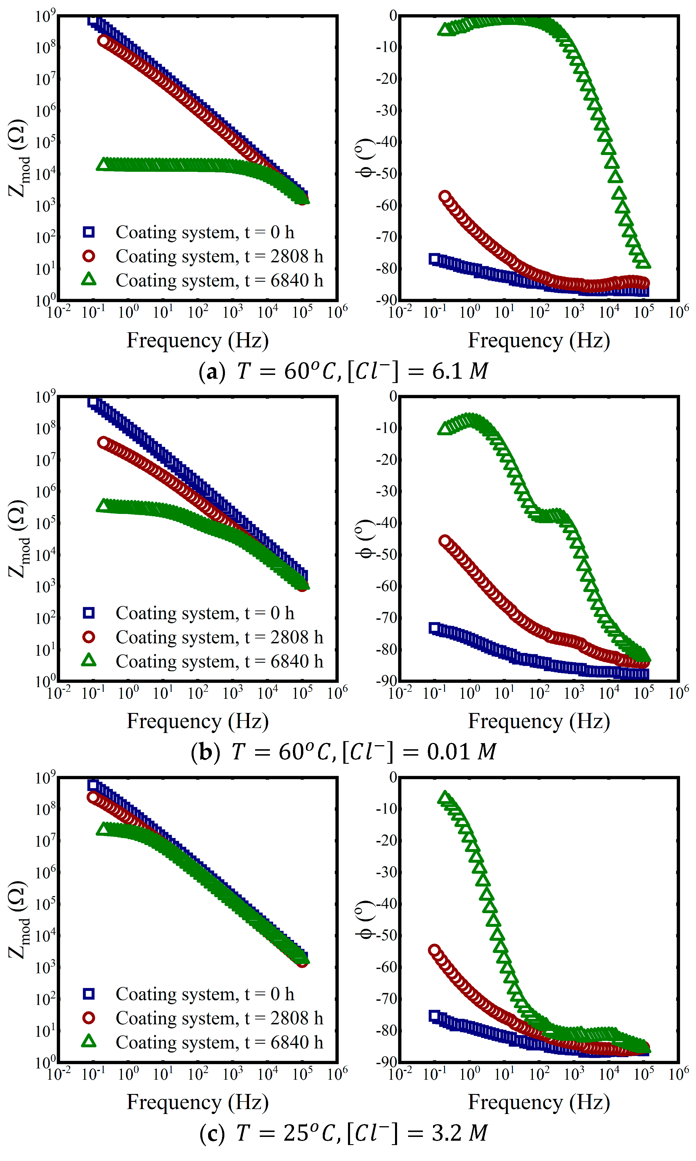
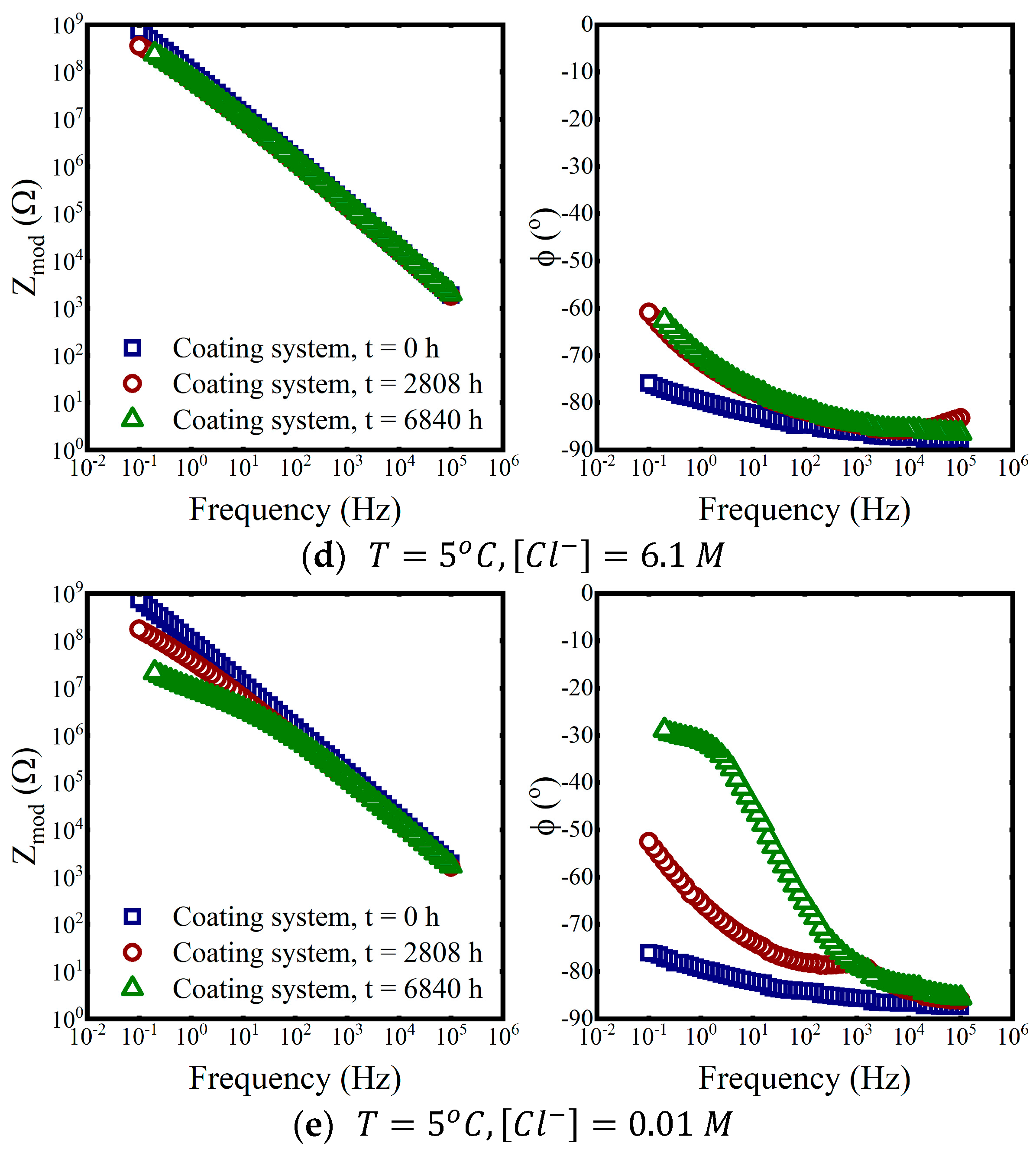
• Immersion in 0.01 M NaCl and saturated NaCl solutions at T = 5 °C and 60 °C;
• Immersion in 3.2 M NaCl at 25 °C.

These immersion conditions were selected to simulate the chemistry of an equilibrated thin film electrolyte in atmospheric exposure conditions ranging from 99% to 70% RH in direct sunlight. Test coupons with coatings were placed in glass beakers that were filled with 1.5 L of the specified solution. Beakers with saturated NaCl solutions contained excess salt to ensure saturation. The beakers were covered with mylar sheets to prevent activity changes from evaporative water loss, and placed in water baths to maintain the specified temperature. The immersion times lasted for approximately 6840 h.

2.2. EIS Measurements and SEM Imaging

Prior to immersion, then approximately halfway through the immersion time, and at the end of the immersion, the coating properties of each coupon were measured using EIS. For the coupons that were immersed, each one was removed from its respective beaker, washed with Type I, ultra-pure, ≥18 MΩ∙cm water (Milli-Q, MilliporeSigma, Burlington, MA, USA), and dried with laboratory-supplied nitrogen. The glass paint test cell (PTC1; Gamry, Warminster, PA, USA) was filled with 40 mL of 0.6 M NaCl and a 3D printed plastic stopper with ports for a reference electrode and counter electrode was used to cap the cell. The exposed area of the coating system was 14.6 cm².

The graphite rod counter electrode and saturated calomel reference electrode (SCE, Gamry) were installed through the plastic stopper so that the distance between the counter and reference electrodes and the working electrode surface was constant for each measurement. The entire assembly was placed inside a Faraday cage to minimize external electrical interference.

The EIS measurements were made in the potentiostatic configuration using a commercial potentiostat (Interface 1000; Gamry, Warminster, PA, USA) with the potential modulated ±10 mV_RMS about the stable potential of the system. The frequency modulation for the potential ranged from 100 kHz to 100 mHz. The frequency values were spaced logarithmically, 10 points per decade, and averaged over 4 cycles at each frequency. The stationary criterion was met with the ±10 mV_RMS perturbation, and linearity of the coupon response to the potential modulation was confirmed using the Kramers-Kronig transform utility provided with the analysis software (Echem Analyst; Gamry, Warminster, PA, USA).

Scanning Electron Microscopy (SEM) samples were created by shearing 1 cm by 3 cm small coupons from the test panel. The small coupons were mounted edge-upward in EpoFix (Struers, Cleveland, OH, USA) epoxy with a 1:1 ratio by weight of conductive nickel filler added (Buehler, Lake Bluff, IL, USA). SEM images and Energy-Dispersive X-ray Spectroscopy (EDS) line profiles were obtained using a Quattro-S environmental SEM (Thermo Fisher, Waltham, MA, USA) in high vacuum mode, operating at either 10 kV for imaging or 20 kV for EDS data collection.

2.3. Theory and Calculations

2.3.1. Review of Equivalent Circuit Modeling for Organic Coatings

The following literature review briefly summarizes important developments in the use of equivalent circuit models for analyzing EIS data obtained from organic coatings. One of its goals is to draw the reader’s attention to the increasing complexity in the equivalent circuit models used to analyze the behavior of coatings. This complexity is seen in the addition of circuit branches and circuit elements to subsequent models as researchers sought improved understanding of features seen in the data from coatings.

The classic review articles by Mansfeld [18] and Murray [19] on using EIS to evaluate coatings were based around employing the “simplified Randles circuit as nested coating defect model” to interpret the electrochemical response of barrier organic coatings exposed to corrosive electrolytes. This equivalent circuit model, shown in Figure 2e, is made up of two building blocks: the undamaged coating circuit model and the simplified Randles circuit model To maintain consistency with the earlier literature, we used the classification scheme shown in Figure 2 to identify equivalent circuit models for interpreting EIS data obtained from coatings. “Modified” describes a version of a circuit model where ideal capacitors have been replaced with constant phase elements. “Simplified” refers to an alteration from the base circuit where the diffusion element has been removed, and “extended” refers to the addition of new circuit elements to a base circuit.

The “undamaged coating circuit” model is shown in Figure 2a. For undamaged coatings, the electrochemical response to an EIS perturbation can be modeled as a resistor-capacitor circuit in series with a resistor. This circuit contains a capacitive element, $C_c$, arising from the dielectric nature of the coating, in parallel with a resistance, R₁, that corresponds with the resistivity of the polymer to electrolytic conduction [20]. The resistance indicated by $R_{\Omega }$ captures conductance losses in the solution between the reference electrode and the coating surface.

Exposure of the coating system to the service, or test environment initiates solution transport through the coating. Pathways for solution transport traditionally have been assigned to the existence of coating defects, such as holidays, or micro-porosity within the polymers that make up the coating system. Wind and Lenderink [21], in their study of the pseudo-Fickian diffusion of water in polymers, noted that it is generally assumed that water permeation into an organic coating occupies the free space between the polymer chains. Coating capacitance is then a measure of the changing mixture of the different dielectric constants of polymer, free space, and water. Once the water reaches the metal-coating interface, the physical system changes again. Beaunier [22] was one of the first to propose that the electrochemical response from a coating defect could be modeled by the addition of a second RC element. This second RC element contains both the charge transfer resistance, R_ct, for faradaic processes occurring at the metal-solution interface, and the electrical double-layer capacitance, $C_{dl}$. These processes, along with diffusion of the reacting species, are contained in the “Randles circuit model” [23], shown in Figure 2c. The “simplified Randles model” omits the diffusion process as a contributor to the impedance.

The “simplified Randles circuit as nested coating defect model”, Figure 2e, has been used extensively to interpret EIS data obtained from organic coatings on metal substrates as a means of assessing the state of the coating [24,25]. However, to address some of the shortcomings from the assumption that the electrical double-layer within the defect acted as a perfect capacitor, Kendig and colleagues substituted a constant phase element (CPE) for the double layer capacitance. This model was called the “Rapid Electrochemical Assessment of Paint (REAP) model” and is shown in Figure 2f [26]. Eventually, the capacitor elements representing both the double-layer and the coating were replaced by CPEs to improve agreement between modeled and measured spectra [27], resulting in the “modified REAP model”, shown in Figure 2g.

Figure 2. Classification of the various equivalent circuit models used for analyzing EIS data obtained from coatings (a) Undamaged coating model [20]; (b) Modified undamaged coating model (this work); (c) Randles model [23]; (d) Modified Randles model (this work); (e) Simplified Randles circuit as nested coating defect model [22]; (f) REAP model [26]; (g) Modified REAP model [27]; (h) Extended modified REAP model (this work, but compare with the equivalent circuits found in [28]).

Figure 2. Classification of the various equivalent circuit models used for analyzing EIS data obtained from coatings (a) Undamaged coating model [20]; (b) Modified undamaged coating model (this work); (c) Randles model [23]; (d) Modified Randles model (this work); (e) Simplified Randles circuit as nested coating defect model [22]; (f) REAP model [26]; (g) Modified REAP model [27]; (h) Extended modified REAP model (this work, but compare with the equivalent circuits found in [28]).

The simplified Randles circuit as nested coating defect model, and its descendants, the REAP and modified REAP models have displayed remarkable longevity as the predominant circuits for evaluating EIS data from organic coatings. This suggests that the relatively simple formulations of these models still represent much of the physical and chemical processes that give rise to the responses measured by EIS experiments. However, excluding the influence of transport processes limits the usefulness of these models for determining the state of the two-layer aircraft coating systems that were studied in this work.

Thus, we propose the “extended modified REAP model”, Figure 2h, founded on the REAP and modified REAP circuits. Like the REAP and modified REAP models, it includes resistive and capacitive elements, in the form of CPEs, but on separate circuit paths for each coating layer. It also includes bounded Warburg elements to represent transport of electrolyte constituents. We hypothesize the extended modified REAP model will provide better insight into the state of a two-layer organic coating system than the other, earlier, models.

Water-uptake by the polymers that make up the coating layers is assumed to underlie the coating behavior that gives rise to most of the equivalent circuit elements seen in the EIS data. Accordingly, in a previous work [29] we developed a numerical model of water uptake by a polymer using the variations in coating dielectric properties over the course of immersion time. That model incorporated expressions for the diffusion coefficient of water uptake as functions of the degree of water saturation of the coating, immersion time, and immersion temperature. We employed that diffusion model in this work as part of the physics-based models for the equivalent circuit element parameters.

2.3.2. Dispersion Relations for Equivalent Circuit Model Elements

Analysis of EIS data using equivalent circuits requires expressions for the dispersion relations for the equivalent circuit elements. These are, in general, straightforward. However, incorporating assumptions about the underlying physical or chemical processes that give rise to the circuit element behavior can provide initial parameter estimates or bounds on the parameter values for the regression algorithm.

Capacitance and Constant Phase Element Models

The impedance for a capacitor that consists of flat, parallel, oppositely charged surfaces, as a function of the angular frequency, $\omega$, is given by (2),

$$Z_c\left(\omega \right)=\frac{1}{Cj\omega },$$

(2)

where $C$ is the capacitance obtained from (3).

$$C=\frac{{ϵ}_i{ϵ}_{0}A}{d},$$

(3)

where $A$ is the exposure area and $d$ is the separation between the oppositely charged regions.

Constant phase elements (CPEs) are generally characterized as non-ideal capacitors because the phase angle of their response is a constant shift that is less than $90°.$ While the underlying mathematical basis for the CPE, arising from a distribution in the dielectric behavior of the material as a function of frequency [30], has long been accepted, the mechanisms that give rise to this behavior have been debated. There have been many attempts at understanding the physical basis for CPE behavior in the electrical double layer at the metal-electrolyte interface. Proposed explanations have ranged from microscopic surface roughness [31] causing differences in capacitance, to phenomena arising from anisotropic fields within the double-layer itself [32,33], to changes in oxide properties arising from different grain orientations of the underlying metal [34]. Hirschorn and colleagues showed that a resistivity distribution within a film can give rise to CPE behavior [35]. Schalenbach and co-authors related the resistivity distribution to ion movement in response to the decaying electric field in the double-layer, and the capacitance contributions of the CPE to charge separation and water molecule polarization [36].

The physical basis for the CPE response from organic polymer coatings has been proposed to arise from a different mechanism. The Concept of Mismatch and Relaxation (CMR) for ion migration in disordered structures by Funke and colleagues [37,38] has been proposed by Abouzari and co-authors to give rise to CPE behavior [39] for polymer coatings.

The impedance as a function of frequency for a CPE is given by (4) [40]

$$Z_{cpe}\left(\omega \right)=\frac{1}{\xi {\left(j\omega \right)}^{\alpha }},$$

(4)

where $\xi$ represents a proportionality factor and $\alpha$ is the CPE exponent. The relationship between $\xi$ and C, for values of $\alpha$ near 1, if the capacitor or constant phase element is part of an RC circuit, is given in (5),

$$\xi =\frac{{\left(C{R}_1\right)}^{\alpha }}{R_1}$$

(5)

where $C$ is the capacitance from (3), and $R_1$ is the resistance of the resistive element.

The capacitance of a polymer changes as a function of water saturation. Prior work has theorized that water uptake by polymers occurs via two principal mechanisms [41]. The first mechanism is a Fickian diffusion process in which water molecules migrate and adsorb at polar sites along the polymer chains [42]. It corresponds to region I on a saturation curve, which is characterized by a steep slope indicating rapidly changing properties with time. The second mechanism is a non-Fickian transport process in which water clusters form and lead to a mixed polymer and water phase [43,44]. This corresponds to region II on a saturation curve, which is characterized by a very shallow slope indicating properties are changing very slowly with time.

Assuming the polymer can be sectioned into thin slices such that each slice has a constant capacitance, the capacitance of each slice is calculated by assuming the dielectric constant of each slice follows the Brasher-mixing law [45]. The overall capacitance can then be obtained as a series combination of individual thin-slice capacitors, as given in (6),

$$\frac{1}{C_c\left(t\right)}=\frac{1}{{Aϵ}_0{ϵ}_{polymer}}{\sum }_{n=1}^N\frac{\mathsf{\Delta }x}{\exp \left(\left({\mathsf{\Psi }}_{\mathrm{n}}\right){\varphi }_{\mathrm{s}}\ln {ϵ}_{H_{2}O}\right)},$$

(6)

where $N$ is the number of slices of thickness $\mathsf{\Delta }x$, ${\varphi }_s$ is the volume fraction of water occupied at saturation, and ${\mathsf{\Psi }}_{\mathrm{n}}$ is the saturation function of each slice, n, and is obtained from the solution to the diffusion Equation (7),

$$\frac{\partial \mathsf{\Psi }\left(x,t\right)}{\partial t}=\frac{\partial }{\partial x}\left(D_{polymer}\frac{\partial \mathsf{\Psi }\left(x,t\right)}{\partial x}\right),$$

(7)

with an initial condition where there is no water present in the coating, a constant Dirichlet boundary condition at the air-coating interface, and a Neumann boundary condition at the coating-metal interface [46]. The diffusivity of the water in the polymer is assumed to change as the mechanism for water uptake changes, with a functional form as given in (8),

$$\begin{array}{c}\mathrm{S}\mathrm{a}\mathrm{t}\mathrm{u}\mathrm{r}\mathrm{a}\mathrm{t}\mathrm{i}\mathrm{o}\mathrm{n} \mathrm{R}\mathrm{e}\mathrm{g}\mathrm{i}\mathrm{o}\mathrm{n} \mathrm{I}:D_{polymer}\left(t\right)=D_I\hfill \\ \mathrm{S}\mathrm{a}\mathrm{t}\mathrm{u}\mathrm{r}\mathrm{a}\mathrm{t}\mathrm{i}\mathrm{o}\mathrm{n} \mathrm{R}\mathrm{e}\mathrm{g}\mathrm{i}\mathrm{o}\mathrm{n} \mathrm{I}\mathrm{I}:D_{polymer}\left(t\right)=\frac{D_{II}}{\left[\frac{\left(D_{II}-D_0\right)}{D_0}\ast e_0^{-D_{II}\frac{t}{A_0}}\right]+1},\hfill \end{array}$$

(8)

where $D_I$ is a constant diffusivity in region I of the saturation curve. $D_{II}$ is the diffusivity in region II of the saturation curve at the end of the mixed water-polymer phase formation and $D_0$ is the diffusion coefficient at the start of the phase formation process. $A_0$ is a characteristic area. The expression for the change in diffusivity in (8) is in the form of an autocatalytic logistic function [47]. Solutions of the diffusion equation with a diffusivity given by (7) can be obtained numerically. Details of the solution are provided elsewhere [29] with the values for ${\mathsf{\Psi }}_n$, then included in (6) to obtain the capacitance.

Resistance Models

The impedance for a resistor, $Z_R$, is dependent on the conductive geometry as indicated in (9),

$$Z_R=R=\frac{\rho l}{A}.$$

(9)

The solution resistance, $R_{\Omega }$, was estimated from (10), using the experimental cell geometry for the distance between the reference electrode and the surface, $l$, and the cross-sectional area, $A$, and the resistivity of the solution, ${\rho }_{c_{C{l}^{-}}}$,

$$R_{\Omega }=\frac{{\rho }_{c_{C{l}^{-}}}l}{A}.$$

(10)

For NaCl solutions at a given temperature and $\left[C{l}^{-}\right]$ concentration, the resistivity was estimated using a Padé approximant model given in (11) [48],

$${\rho }_{\left[C{l}^{-}\right]}={\left[\frac{\left(0.0480+0.0034T\right)+\left(6.7545+0.2392T\right)\left[C{l}^{-}\right]}{1.0+\left(0.2065+0.0013T\right)\left[C{l}^{-}\right]}\right]}^{-1},$$

(11)

where $T$ is the temperature in Celsius and $c_{C{l}^{-}}$ is the chloride concentration in mol/L.

For $T=25°\mathrm{C}$, $\left[C{l}^{-}\right]=0.6\mathrm{M}$, $A=14.96\mathrm{c}{\mathrm{m}}^2$, and $l=4\mathrm{c}\mathrm{m}$, the value obtained from (11) was $3.92\Omega$. When compared with the high-frequency impedance data from the as-received and pre-treated alloys, $4.07\Omega$ and $4.16\Omega$, respectively, the calculated value from the model differed from the EIS analysis value by less than 6%.

The model for the resistance of the polymer coatings employed several simplifying assumptions to abstract the complex physical processes occurring within the polymer. For water uptake in the first region of the saturation curve, the resistance of the polymers was assumed to function as two resistors in series: the wetting or saturated polymer and the dry polymer. This is represented in (12),

$$R_{t,p}=\frac{{\rho }_e{d}_e}{A}+\frac{{{\rho }_{p}d}_d}{A},$$

(12)

where $d_e$ corresponds to the depth of water penetration, ${\rho }_e$ is the resistivity of the electrolyte solution, ${\rho }_p$ is the resistivity of the polymer, and $d_d$ is the remaining depth of the polymer. The two depths are related to one another by (13),

$$d_d=L-d_e,$$

(13)

where $L$ is the coating layer thickness. The resistivity of the epoxy and polyurethane was obtained from the functional fits plotted in Figure 3a,b, respectively. The models for the resistivity changes as a function of water uptake follow the approach taken by Lutz and co-workers [49] with data from the literature [49,50].

Both volume resistivity models are exponential decay functions of the form given in (14),

$$\rho =\frac{\left(c_1{e}^{-c_2\mathsf{\Psi }}\right)}{a_1{e}^{{-a}_2\mathsf{\Psi }}+e^{-b\mathsf{\Psi }}},$$

(14)

where the saturation function, $\mathsf{\Psi }={\varphi }_{H_{2}O}/{\varphi }_{H_{2}O}^{sat,99\%}$ and the parameter values given in

Table 1. Parameter values for calculating volume resistivity.

Parameter	Epoxy	Polyurethane
a1	5.32 × 10−21	4.08 × 10−7
a2	5.10	10.61
b	63.34	30.07
c1	3.40 × 1045	4.18 × 1031
c2	68.44	40.67

were obtained from regression fits to the data points.

Diffusion Impedance Models

The resistance values obtained from (14) were assumed to dominate the in-phase impedance response until continuous electrolyte pathways existed between the coating-electrolyte interface and coating-oxide interface. Once these pathways were established, we assumed that the mass transport impedance arising from the transport of electrolyte species became the principal contributor to the resistance. This impedance is obtained using (15) [51], for the bounded Warburg element,

$$Z_W\left(\omega \right)=\frac{\sqrt{2}\sigma }{\sqrt{j\sigma }}\tanh \left(\frac{\delta \sqrt{j\omega }}{\sqrt{D}}\right)$$

(15)

where $\sigma$ is the Warburg coefficient. Values for $\sigma$ were obtained from (16),

$$\sigma =\frac{RT}{{\sqrt{2}\left(zF\right)}^{2}A}\left[\frac{1}{c_O^b\sqrt{D_{eff,O}}}+\frac{1}{c_R^b\sqrt{D_{eff,R}}}\right]$$

(16)

where $c_O$ indicates the concentration of the oxidized species, $c_R$ is the concentration of the reduced species, $D_{eff,i}$ is the effective diffusivity of the oxidized or reduced species, $A$ is the exposure area, Faraday constant, $F=\mathrm{96,485}\mathrm{C}/\mathrm{m}\mathrm{o}\mathrm{l}$, $z$ is the ionic charge, and $c_i^b$ represents the bulk solution concentration.

If we assume a redox reaction at the primer-pretreatment interface is the principal contribution to the Warburg coefficient, then in this case, the likely redox reactions are either oxygen reduction or water reduction. In the case of oxygen reduction, dissolved oxygen needs to diffuse from the bulk electrolyte through the coating to the oxide-coating interface, where it is reduced to form hydroxide ions. For water reduction, the water molecules participating in the water uptake process are reduced at the oxide-coating interface. While the second mechanism provides a simpler explanation, our data is insufficient to distinguish which redox reaction is occurring.

This approach differs slightly from the analysis performed by Skale and colleagues [52]. In this earlier work, a Dirichlet boundary condition was assumed at the coating-substrate interface, so the diffusion impedance was modeled as a semi-infinite Warburg element. However, to solve (7), our approach assumed a Neumann boundary condition at the oxide-coating interface, which resulted in a bounded Warburg element for the diffusion impedance. This is similar to the equivalent circuit models developed by Volmajer and colleagues [53] for the analysis of EIS data obtained during curing epoxy coatings. In our case, the presence of the two different organic polymers that make up the coating system also required the addition of a second bounded Warburg element circuit.

The average diffusivity of the electrolyte constituents inside the coating is assumed to differ from the bulk diffusivity in the electrolyte. In our case, we assumed the transport of the electrolyte components occurred only along the polymer chains. Thus, the complex shapes of filler and pigment particles, from the cross-section of the coating system shown in Figure 1 formed a solid matrix and the polymer regions were assumed to consist of a mix of solid and void space. We used the continuum approximation given in (17) [54] to relate the notional porosity of the polymer film to a Darcy-equivalent, $D_{eff}$[55],

$$D_{eff}=\frac{ϵD_b}{\tau }$$

(17)

where $ϵ$ is a measure of the porosity, $D_b$ is the bulk diffusivity value, and, from the Bruggeman relation [56], $\tau =1.0/\sqrt{ϵ}$. This empirical approach does neglect interactions between the electrolyte ions and the polymer structure [57]; however, it simplifies the effective diffusivity model.

2.3.3. Derivation of Conductivity Matrices for Equivalent Circuit Models

The derivation of the conductivity matrix for the modified undamaged coating equivalent circuit model starts with Kirchhoff’s current law in (18) for each branch of the circuit,

$$\Sigma i_k=0,$$

(18)

$$i_3=i_1+i_2,$$

(19)

where $i_3$ is the current flowing through $R_{\Omega }$, $i_2$ is the current flowing through the CPE, and $i_1$ is the current flowing through $R_1$.

As in most other electrical circuit analyses, the fundamental building block for determining the impedance of a circuit is Ohm’s Law. The frequency-dependent impedance of a circuit can be expressed using (20) [58],

$$e_0\sin \omega t=\left(i_0\sin \omega t+\varphi \right)Z\left(\omega \right)$$

(20)

where $\omega =2\pi f$, $f$ is the oscillation frequency, $e_0$ is the amplitude of the sinusoidal potential oscillation, $i_0$ is the amplitude of the current response, and $\varphi$ is the phase shift in the current.

Using (20), expressions for the sum of the voltage drops through both pathways in the circuit are given in (21),

$$\begin{gathered} v_1=i_3{R}_{\Omega }+i_1{R}_1, \\ {v}_2=i_3{R}_{\Omega }+i_2{Z}_{cpe}. \end{gathered}$$

(21)

Then using (19) to substitute for $i_3$ and collecting terms results in (22),

$$\begin{gathered} v_1=i_1\left(R_{\Omega }+R_1\right)+i_2{R}_{\Omega }, \\ {v}_2=i_1{R}_{\Omega }+i_2\left(R_{\Omega }+Z_{cpe}\right). \end{gathered}$$

(22)

Rewriting the system of equations from (22) in matrix form results in (23),

$$\left[\begin{array}{c}{v}_1\\ v_2\end{array}\right]=\left[\begin{array}{c}{i}_1\\ i_2\end{array}\right]\left[\begin{array}{cc}{R}_{\Omega }+R_1& R_{\Omega }\\ R_{\Omega }& R_{\Omega }+Z_{cpe}\end{array}\right],$$

(23)

where the conductivity matrix is given by (24),

$$\mathit{Z}=\left[\begin{array}{cc}{R}_{\Omega }+R_1& R_{\Omega }\\ R_{\Omega }& R_{\Omega }+Z_{cpe}\end{array}\right].$$

(24)

The circuit models shown in Figure 2 can be divided into three categories: 2, 3, and 4 pathway models. The circuits from Figure 2a–d are 2-pathway models, while the circuits from Figure 2e–g are 3 pathway models, and the circuit in Figure 2h is a 4-pathway model. The number of pathways indicates the number of rows and columns in the conductivity matrices that are constructed for the impedance calculations, and the number of rows and columns in the conductivity matrix in (24) are consistent with a 2-pathway equivalent circuit.

The modified Randles circuit is also a 2-pathway equivalent circuit. The conductivity matrix is given in (25) and was derived using a similar procedure as shown previously.

$$Z=\left[\begin{array}{cc}{R}_{\Omega }+R_1+Z_W& R_{\Omega }\\ R_{\Omega }& R_{\Omega }+Z_{cpe}\end{array}\right]$$

(25)

The extended modified REAP equivalent circuit model, introduced in this work, and shown in Figure 2h, is a 4-pathway equivalent circuit. This circuit was derived from the previous equivalent circuits that have been used for analyzing EIS data from coating systems. This circuit is intended to account for effects from non-ideal capacitive behavior and transport of electrolyte species in different coating layers, as well as electrochemical processes occurring at the coating-substrate interface. The conductivity matrix is given in (26).

$$\begin{gathered} Z=\left[\begin{array}{cccc}{Z}_{00}& Z_{01}& Z_{02}& Z_{03}\\ Z_{10}& Z_{11}& Z_{12}& Z_{13}\\ Z_{20}& Z_{21}& Z_{22}& Z_{23}\\ Z_{30}& Z_{31}& Z_{32}& Z_{33}\end{array}\right] \\ {Z}_{00}=R_{\Omega }+R_t+Z_W^t+R_p+Z_W^p+R_{pre} \\ {Z}_{11}=R_{\Omega }+R_t+Z_W^t+R_p+{Z_W^p+Z}_{cpe}^{pre} \\ {Z}_{22}=R_{\Omega }+R_t+Z_W^t+Z_{cpe}^p \\ {Z}_{33}=R_{\Omega }+Z_{cpe}^t \\ {Z}_{01}=Z_{10}=R_{\Omega }+R_t+Z_W^t+R_p+Z_W^p \\ {Z}_{02}=Z_{20}=Z_{21}=Z_{12}=R_{\Omega }+R_t+Z_W^t \\ {Z}_{03}=Z_{30}=Z_{13}=Z_{31}=Z_{23}=Z_{32}=R_{\Omega } \end{gathered}$$

(26)

2.3.4. Algorithm for Determining the Frequency-Dependent Impedance of an Equivalent Circuit Model

To determine the impedance at each frequency, the following algorithm was employed:

• The currents flowing in each path of the circuit were calculated from (27),

$$i=Z^{-1}v.$$

(27)

The solution to (27) was obtained using an LU decomposition algorithm from the mldivide function in MATLAB (R2023a, MathWorks) because the conductivity matrices are square matrices with only a few elements.

• The M individual current components of the $i$ vector from (27) were then summed to obtain the total current,$i_t$, as shown in (28),

  $$i_t=\sum _{m=0}^{M-1}{i}_m.$$

  (28)

• Regardless of the path through the circuit, the voltage drop across each path must be the same and, for convenience, we assumed $v_m=e_0=1.0$. The complex impedance at each frequency was then obtained from (29),

$$Z\left(\omega \right)=\frac{e_0}{i_t}=x+jy,$$

(29)

where $x$ and $y$ are the calculated real and imaginary components of the impedance, respectively, and $j=\sqrt{-1}$.

2.3.5. Procedure for Fitting Model Impedance to EIS Data

Fits to the experimental data were obtained by a simplex regression algorithm [59,60] coded in MATLAB (R2023a, MathWorks). The regression algorithm minimized the value of the mean squared error (MSE) between model results and experimental data. The error calculation was dependent on both the number of data points measured and the number of parameters, as given in (30) [61],

$$MSE=\frac{\left[\sum _{i=1}^N\left({\left(\frac{u_i-x_i}{x_i}\right)}^2+{\left(\frac{v_i-y_i}{y_i}\right)}^2\right)\right]}{N-k}$$

(30)

where $u_i+j{v}_i$ represents one of N complex data points, $x_i+j{y}_i$ represents a complex point obtained from the model, and $k$ represents the number of parameters in the model.

The regression procedure was executed in the following manner:

• Bound the upper and lower fitting parameter values to prevent non-physical results, such as negative resistances.
• Use the simplex method to perform the regression of the equivalent circuit model to the data.
• Generate a set of 1000 vertices in the k parameter space.
• The first vertex uses the initial estimate parameter set.
• The second vertex consists of the lower bound of parameter values.
• The last vertex consists of the upper bound of parameter values.
• The remaining vertices consist of randomly generated values spanning the range between the upper and lower bounds [61].
• Calculate the MSE for each vertex.
• Create the first simplex from the k+1 vertices that have the lowest MSE.
• Start the regression and iterate using reflection, contraction, or extension on the vertex with the highest MSE in the simplex to keep or reject that vertex. This forms a new simplex.
• Continue iterating until the convergence criterion is satisfied or the number of iterations exceeds the maximum allowed.
• Repeat the regression 32 times. Because of the randomly formed middle vertices, this can result in different vertices in the initial simplex, which can result in a slightly different convergence. Of the 32 outcomes, select the parameter values from the simplex that resulted in the lowest MSE.

3. Results

3.1. EIS Measurements of the Initial Coating Layers

EIS measurements were made on as-received aluminum alloy panels, pretreated panels, primer-only panels, and coating system panels prior to immersion. Representative examples of these results are plotted on Bode diagrams, with the logarithm of the impedance modulus, $Z_{mod}$, and phase angle, $\varphi$, as functions of the logarithm of the frequency in Figure 4. Nyquist plots are also frequently used for representing EIS data for many biological systems, especially when employing graphical analysis methods [62,63,64]. However, in the case of commercial coating systems, with impedance values in the $M\Omega$ to $G\Omega$ range, high-frequency features of the data are obscured because Nyquist plots use linear scales.

3.2. EIS Measurements of the Immersed Coatings

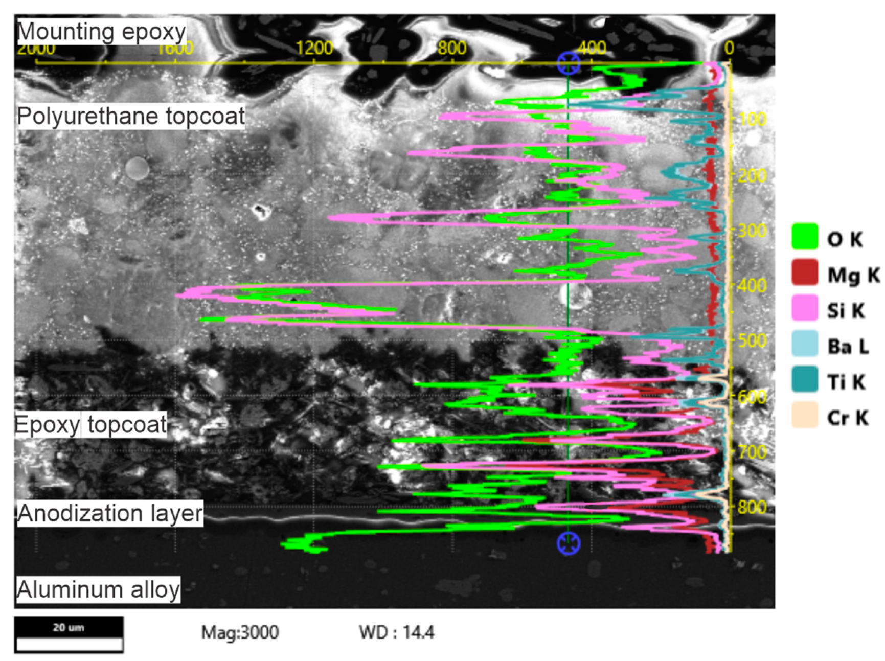
EIS measurements were made at the start of the exposure, t_immersion = 0 h; approximately halfway through at t_immersion = 2808 h; and at the end of the exposure period, t_immersion = 6840 h. Representative examples of the data for all immersion conditions are shown in Figure 5. The EIS data is plotted using the Bode representation with $Z_{mod}$ and the phase angle plotted versus the oscillation frequency.

The EIS data was analyzed by fitting to the various equivalent circuit models found in Figure 1 using the EIS Analysis software suite written in MATLAB (Version R2023a, MathWorks). The parameters from the models were then correlated with the physical and chemical processes occurring in the coating systems.

The stationary criterion for EIS analysis was met on the coated coupons with the ±10 mV_RMS perturbation. For these measurements, the linearity of the coating systems’ responses to the 28-mV peak-to-peak potential perturbation was confirmed using the Kramers-Kronig transform utility provided with the analysis software (Echem Analyst; Gamry, Warminster, PA, USA) for the potentiostat.

3.3. SEM Analysis

Figure 6 shows a cross-section of the coating system with the individual layers identified. The EDS line scan shows the relative concentrations of the various elements and provides an indication of the fillers and additives in each coating layer. The chromate inhibitor additives are found only in the primer. In this sample, the polyurethane topcoat had an average thickness of $41.9\pm 3.0\mathsf{\mu }\mathrm{m}$, while the epoxy primer had an average thickness of $19.9\pm 3.7\mathsf{\mu }\mathrm{m}$. The pretreatment layer had an average thickness of $7.9\pm 1.6\mathsf{\mu }\mathrm{m}$. The complex structures of the individual coating layers justified the representation of the diffusivities as effective diffusion coefficients, dependent on the tortuosity and porosity of the polymers.

Attempts to determine the sodium and chloride concentrations between the two layers, and among samples immersed in the different solutions, were inconclusive. The line scans of these elements did not show clear trends, which is likely due to the depth of the interaction volume from the electron beam.

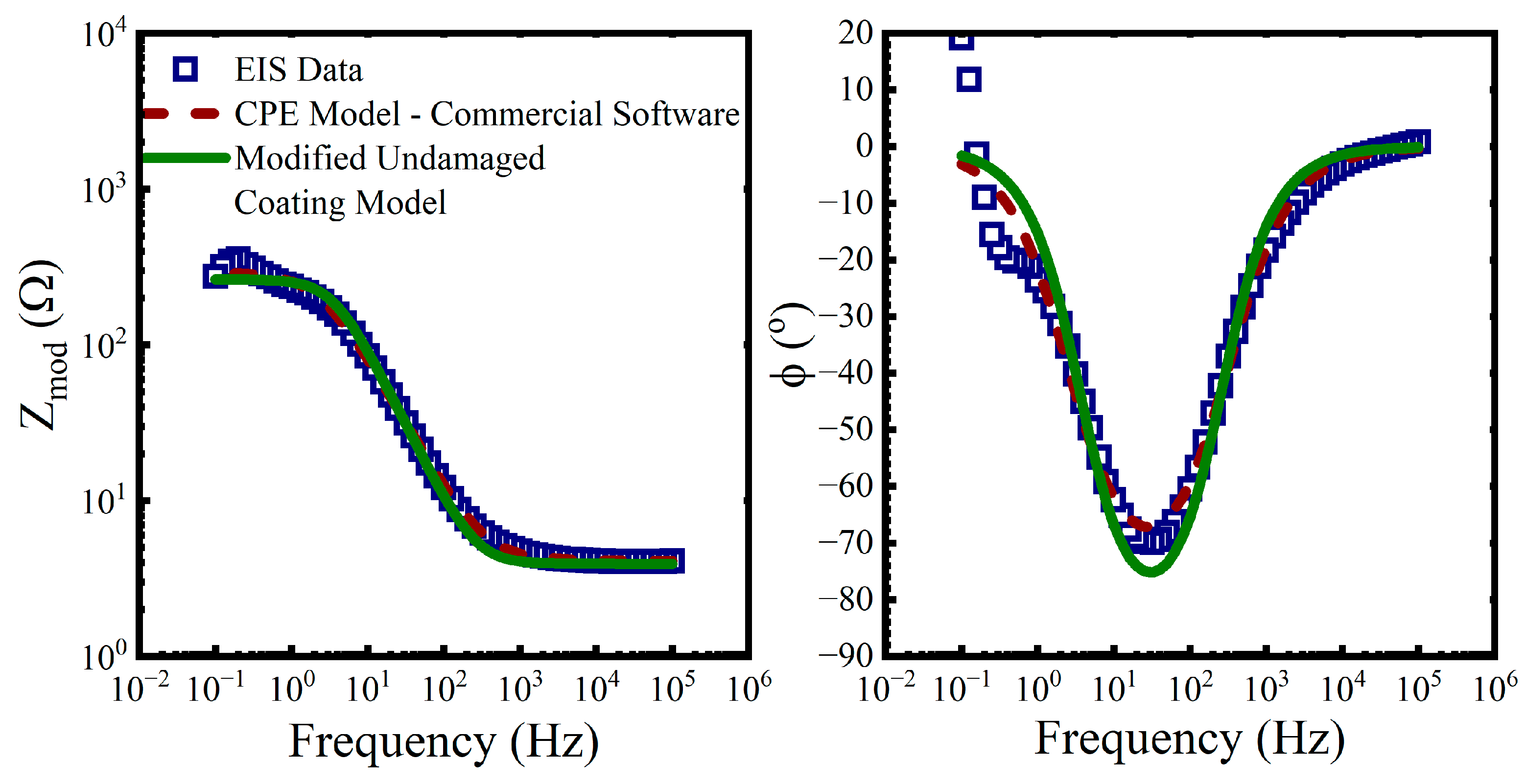
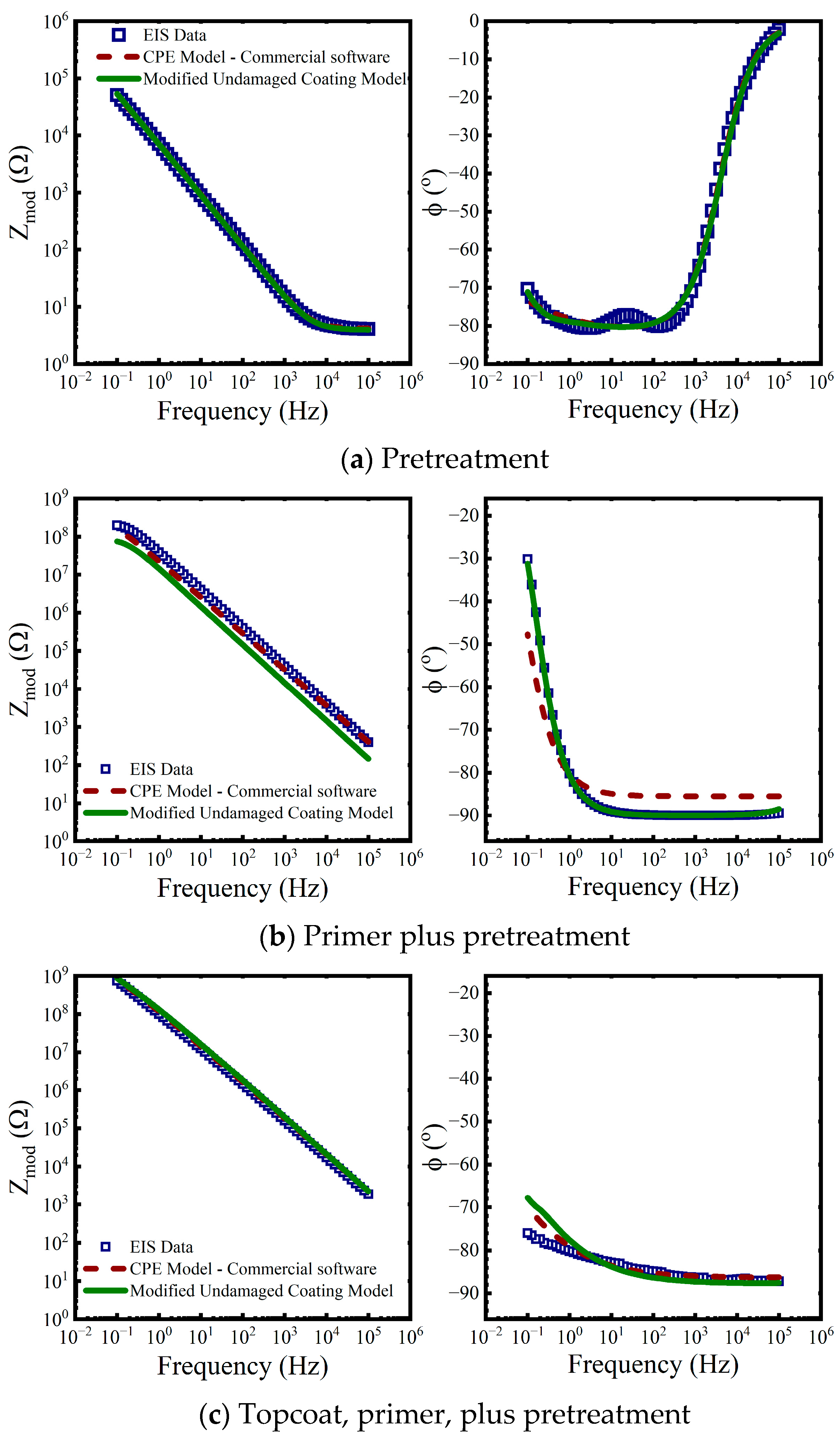
3.4. Fits Using the Modified Undamaged Coating Circuit

The modified undamaged coating circuit model replaced the capacitor in the single RC circuit of the undamaged coatings model with a constant phase element. This circuit, from Figure 2b, was fit to the as-received oxide data, shown in Figure 4a. The fit values and MSE are given in

Table 2. Equivalent circuit parameter values for the as-received oxide at $T={25}^{o}C$ and $\left[C{l}^{-}\right]=0.6\mathrm{M}$.

Parameter	Equivalent Circuit Model Used for the Analysis
	Modified Undamaged Coating	CPE Model Commercial Software
$R_1\left(\Omega ·{\mathrm{c}\mathrm{m}}^2\right)$	$3875$	$4338$
$\xi \left(\frac{\mathsf{\mu }\mathrm{F}}{{\mathrm{c}\mathrm{m}}^2}·{\mathrm{s}}^{\alpha -1}\right)$	$11.6$	$19.5$
$\alpha$	$0.990$	$0.891$
${\mathrm{R}}_{\Omega }(\Omega )$	3.92	4.01
MSE	0.362	$0.861$

.

Table 2 also shows values obtained from fitting the data using a commercial software package (Echem Analyst Ver. 7, Gamry, Warminster, PA, USA) and the included CPE equivalent circuit model. MSE values are included for comparison because that is the statistic the commercial software used to determine goodness of fit. The predicted impedance values for the modulus and phase for the two models are plotted in Figure 7 along with the measured data.

Comparing the circuit element values between the two models in Table 2 and visually in Figure 7 suggests that both approaches for modeling the impedance of the equivalent circuit result in similar outcomes.

3.5. Fits Using the Modified Randles Circuit

While the modified undamaged coating circuit model was effective at fitting the EIS data from the as-received AA2024, it resulted in poor fits for the other baseline EIS data shown in Figure 4b–d. For these fits, we used the modified Randles circuit model. Parameter values for this circuit were obtained by using the conductivity matrix in (25) and the fitting procedure to analyze the EIS data from the pretreated layer, the primer coating, and the topcoat.

The fit values for the circuit parameters are provided in

Table 3. Equivalent circuit parameter values for the coating layers at $T=25 °\mathrm{C}$ and $\left[C{l}^{-}\right]=0.6\mathrm{M}$.

	Equivalent Circuit Model Used for the Analysis
	Modified Randles Circuit			CPE with Diffusion Commercial Software
Parameter	Oxide	Primer	Topcoat	Oxide	Primer	Topcoat
$R_1\left(\mathrm{M}\Omega ·{\mathrm{c}\mathrm{m}}^2\right)$	$0.084$	$3440$	$0.15$	$0.063$	$3590$	$0.04$
$\xi \left(\frac{\mathrm{n}\mathrm{F}}{\mathrm{c}{\mathrm{m}}^2}·{\mathrm{s}}^{\mathsf{\alpha }-1}\right)$	$1670$	$0.27$	$0.07$	$1600$	$0.52$	$0.08$
$\alpha$	$0.91$	$0.99$	$0.97$	$0.91$	$0.95$	$0.96$
$\sigma \left(\frac{\mathrm{M}\Omega ·{\mathrm{c}\mathrm{m}}^2}{\sqrt{\mathrm{s}}}\right)$	$2.39$	$0.15$	$\mathrm{13,500}$	$3.44$	$0.06$	$\mathrm{32,600}$
MSE	$0.02$	$0.25$	0.04	$0.001$	0.16	0.001

. Table 3 also shows values obtained from fits using a commercial software package (Echem Analyst Ver. 7, Gamry) and the included CPE with diffusion circuit model. Comparisons for the predicted impedance values for the modified Randles model and CPE with diffusion equivalent circuit model are plotted in Figure 8.

Again, comparing the circuit parameter values between the two modeling approaches in Table 3 suggests that both approaches arrive at similar outcomes. However, there is a shortcoming with both approaches. The upper and lower bounds on the parameter values used in the simplex regression algorithm were arbitrarily selected rather than arising from our understanding of the physical and chemical processes at work in the coating system.

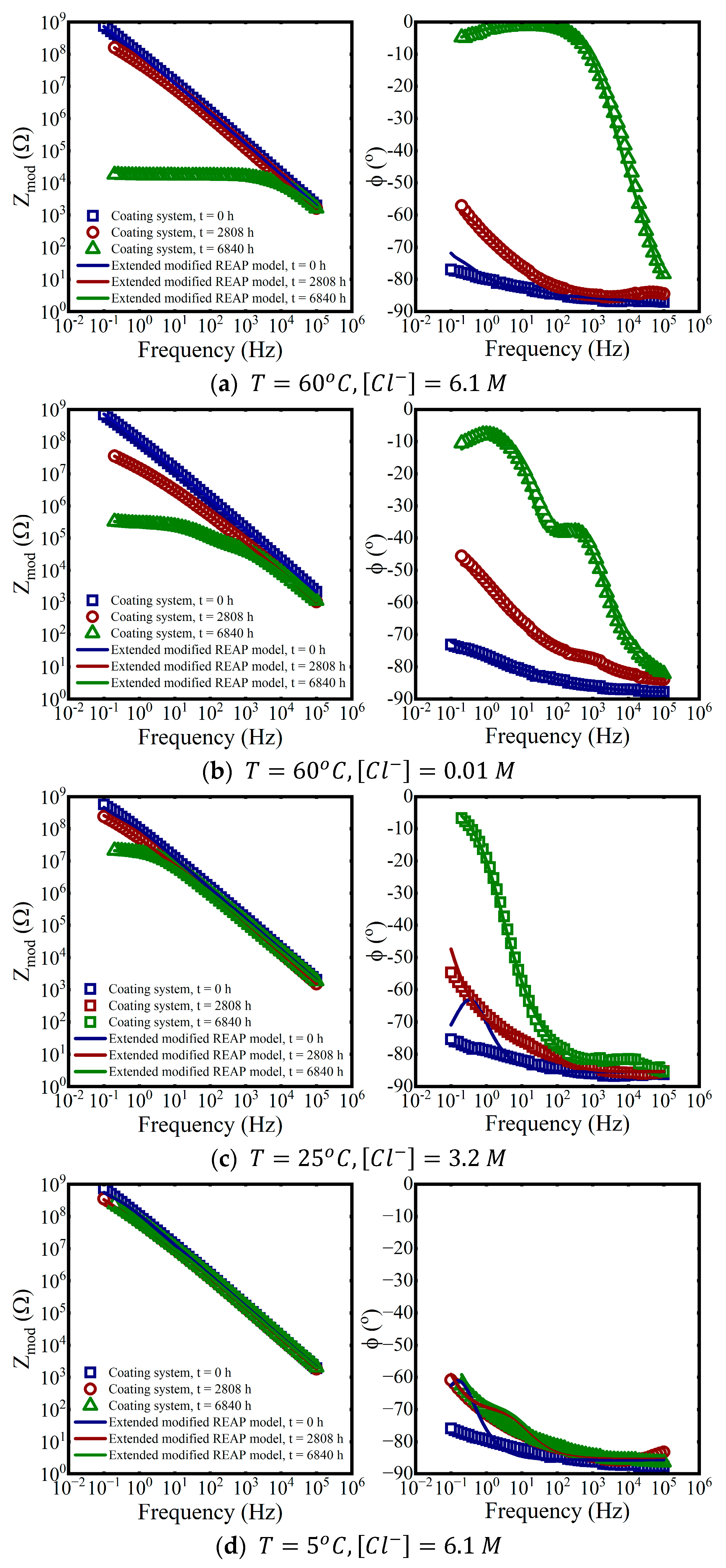
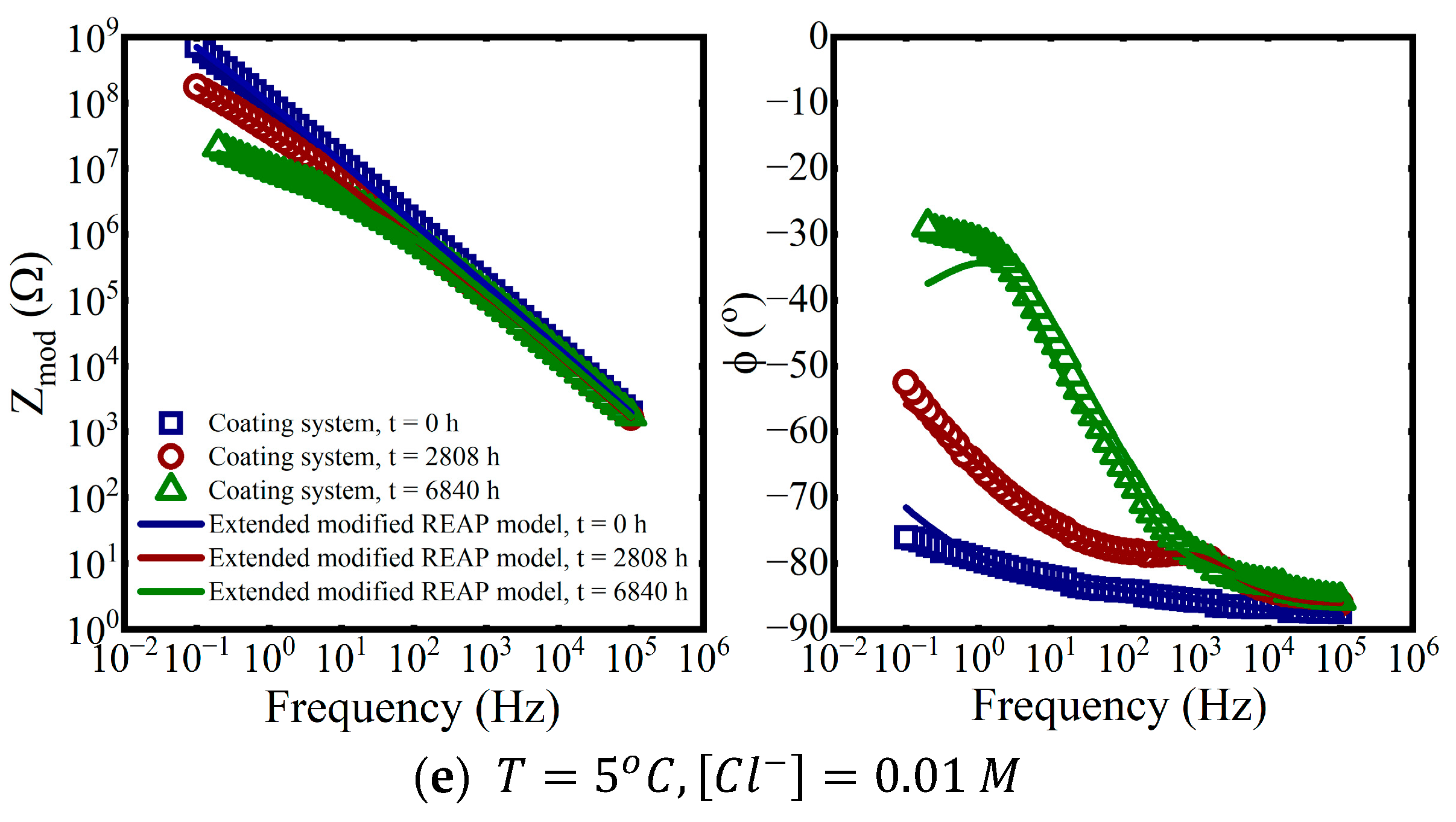
3.6. Fits Using the Extended Modified REAP Circuit

The expressions in (4) and (17) allowed us to estimate initial values for some of the circuit elements from these physics-based models. Thus, the first step in the nonlinear regression procedure was modified to the following:

• Create an initial estimate of the equivalent circuit parameters from the physics-based models. For the baseline measurements of the as-received and pretreated samples, the charge-transfer resistance was treated as a fit parameter. These values became the initial guesses for those parameters in this procedure.
• Solve the diffusion equation for water saturation for the given immersion time with diffusion coefficients obtained from (8).
• Use (6) and (14) to estimate the coating layers’ capacitance and resistance, respectively.
• Estimate the impedance of the Warburg elements from (15). We assumed the dissolved oxygen diffusivity and concentration were functions of temperature and chloride concentration and allowed the diffusion length to vary as a fit parameter.

Figure 9 shows an example comparison between the impedance obtained from the physics-based models’ initial parameter estimates and the impedance after the regression.

The results of fits using the extended modified REAP model for all immersion conditions are shown in Figure 10.

An example of the parameter values for the coating system immersed in 3.2 M NaCl at 25 °C for 2808 h is shown in

Table 4. Equivalent circuit parameter values for the coating layers at $T=25°\mathrm{C}$ and $\left[C{l}^{-}\right]=3.2\mathrm{M}$. Shaded rows indicate different coating layers.

Layer	Parameter	Value
Electrolyte	$R_{\Omega }\left(\Omega \right)$	$3.93$
Topcoat	$R_T\left(\mathrm{k}\Omega ·{\mathrm{c}\mathrm{m}}^2\right)$	$16.0$
	${\xi }^T\left(\frac{\mathrm{p}\mathrm{F}}{\mathrm{c}{\mathrm{m}}^2}·{\mathrm{s}}^{\alpha -1}\right)$	$66.8$
	${\alpha }_T$	$0.99$
	${\sigma }_T\left(\frac{\Omega ·{\mathrm{c}\mathrm{m}}^2}{\sqrt{\mathrm{s}}}\right)$	$212.4$
	$D_{eff}^T\left(\frac{{\mathrm{m}}^2}{\mathrm{s}}\right)$	$4.93\times {10}^{-13}$
Primer	$R_P\left(\mathrm{M}\Omega ·\mathrm{c}{\mathrm{m}}^2\right)$	$28.9$
	${\xi }^P\left(\frac{\mathrm{p}\mathrm{F}}{\mathrm{c}{\mathrm{m}}^2}·{\mathrm{s}}^{\alpha -1}\right)$	$90.9$
	${\alpha }_P$	$0.85$
	${\sigma }_P\left(\frac{\mathrm{G}\Omega ·{\mathrm{c}\mathrm{m}}^2}{\sqrt{\mathrm{s}}}\right)$	$3.0$
	$D_{eff}^P\left(\frac{{\mathrm{m}}^2}{\mathrm{s}}\right)$	$3.08\times {10}^{-15}$
Pretreatment	$R_{pre}\left(\Omega ·\mathrm{c}{\mathrm{m}}^2\right)$	$149.6$
	${\xi }^{DL}\left(\frac{\mathrm{p}\mathrm{F}}{\mathrm{c}{\mathrm{m}}^2}·{\mathrm{s}}^{\alpha -1}\right)$	$304$
	${\alpha }_{DL}$	$0.90$
	MSE	$0.006$

.

As expected, the CPE parameter values for both coating layers are consistent with water uptake by the polymers. The water uptake increases the dielectric constants for both materials above their dry values, which results in a higher capacitance.

The $R_T$ and $R_P$ values approximating the pore resistances of the coating suggest that continuous electrolyte paths exist from the solution to the coating-oxide interface. However, the bounded Warburg coefficient value, ${\sigma }_P$, for the epoxy primer suggests that the primer is still providing good barrier protection for the substrate.

The effective diffusion coefficient listed in Table 4 for the topcoat is consistent with the literature values of the diffusion coefficient for water molecules in polyurethane $\left(5.0\times {10}^{-13}{\mathrm{m}}^2/\mathrm{s}\right)$ [65]. This value, in combination with the Warburg coefficients, suggests relatively easy transport for all electrolyte species through the polyurethane topcoat at this point in the immersion, as diffusion of O₂ and H₂O molecules is higher than the other species. In contrast, $D_{eff}^P$ in the primer layer is much lower than the expected water diffusion coefficient in epoxy $\left(3.5\times {10}^{-13} {\mathrm{m}}^2/\mathrm{s}\right)$ [49]. Instead, $D_{eff}^P$ is more consistent with Na⁺ or Cl⁻ ion transport $\left(3.1\times {10}^{-15}, 4.7\times {10}^{-16} {\mathrm{m}}^2/\mathrm{s}\right)$, respectively [5]. This suggests that, for the epoxy primer, electrolyte ion transport is the principal charge carrier.

While the charge-transfer resistance at the oxide-coating interface is low, the CPE coefficient and exponent indicate the anodized pretreatment is still stable. This is consistent with the fit results for the diffusion coefficients. It has been suggested that Na⁺ ion transport is the principal ionic charge carrier in coatings, and it is the chief contributor to the charge balance at cathodic sites at the coating-substrate interface [4]. It is likely that Na⁺ and Cl⁻ ions are still migrating through the coating and have not reached sufficient concentration to disrupt the thickened oxide.

4. Discussion

4.1. Justification for Using the Extended Modified REAP Model

Each equivalent circuit model from Figure 2 was fit to an experimental data set obtained from a coating system immersed in 0.01 M NaCl at 60 °C for 2808 h. This coating system exhibited a large change in $Z_{mod}$ over the duration of the immersion, as shown in Figure 10b, so it was deemed to be a good candidate by which to evaluate the candidate equivalent circuit models. The models were regressed to the data set using the simplex regression algorithm using similar initial guesses. The outcomes of the fits are shown in Figure 11.

The calculated MSEs for the fits in Figure 11, along with the number of independent parameters, k, are shown in

Table 5. MSE and AICc values for the various equivalent circuits fit to the same data.

Circuit Name	MSE	k	AICc
Undamaged coatings model	3.82	2	589.85
Modified undamaged coatings model	0.13	3	173.79
Randles model	130.64	5	1021.75
Modified Randles model	0.13	6	181.11
Simplified Randles circuit as nested coating defect model	140.66	4	1030.36
REAP model	149.24	5	1037.99
Modified REAP model	0.13	6	181.39
Extended modified REAP model	0.005	16	−216.79
Voigt elements model	$6.0\times {10}^{-6}$	58	6578.69

. The last circuit listed corresponds to 29 Voigt elements, a resistor and capacitor in parallel with one another. Because there are two parameters to a Voigt element, a resistance and capacitance, this represents the maximum number of circuit elements that could be fit to the data. We assume this also sets the minimum MSE value.

The MSE results for the circuits based around the undamaged coating model have similar values and are quite high, indicating that the fits are poor. This is due to two reasons:

• The inability of the capacitance to capture deviations from −1 in $\mathsf{\Delta }\log Z_{mod}/\mathsf{\Delta }\log f$ that arise because the coatings and oxide functioned as imperfect capacitors.
• The lack of a diffusion-influenced impedance element in these models.

In purely numerical terms, the presence of CPE and Warburg elements increases the number of parameters available for the regression routine, thereby reducing the MSE. Pursuing the lowest MSE value, however, illustrated by an equivalent circuit consisting entirely of Voigt elements, provides little physical insight into the state of the coating. So, rather than basing model selection for fitting the coating data on the MSE, we used the corrected Akaike information criterion [66] (AICc) as the statistic for this selection. The corrected AIC helps to account for model overfitting due to small sample sizes. The AICc can be calculated by (31) [67],

$$AICc=k+\left(N\left(2\pi \ast MSE\right)+1\right)+\left(\frac{2k^2+2k}{k-N-1}\right).$$

(31)

In (31), as the number of data points, $N\to \infty$, $AICc\to 0$ and the expression reverts to the classic AIC statistic.

The AICc values for the equivalent circuit fits are given in the last column of Table 5. Like the MSE, lower values are better in terms of evaluating the model. The corrected AIC statistic severely penalizes the Voigt elements circuit but suggests the extended modified REAP circuit does not overfit the data while still providing a low MSE.

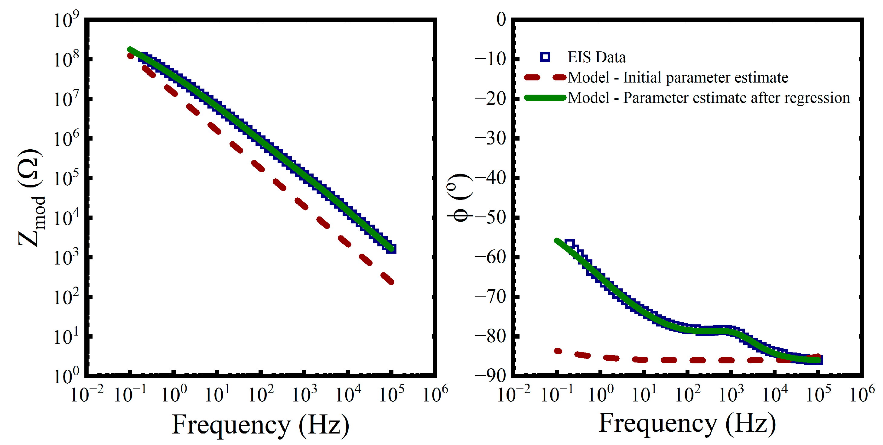
4.2. Imposing Physical Constraints in the Regression Algorithm

The regression algorithm outlined in Section 2.3.5 used physics-based equations to obtain starting values for the fits, but the constraints on the parameter values were minimal. Specifically, negative parameter values were rejected, and resistance values were capped at ${10}^{10}\Omega$. However, from a physical standpoint, including circuit elements such as the CPE and Warburg that can represent more complex behavior in the coating than resistors and capacitors suggests that additional constraints can be obtained from our understanding of coating behavior. That is, we can impose the following physical constraints on the system:

• Coating layer resistance, while initially high, is expected to drop rapidly during immersion because of water uptake, as shown in (14);
• Inversely, coating capacitance, while initially low, will increase as a function of water saturation, as suggested by (6);
• The Warburg elements will impact the impedance once a continuous diffusion path exists for the reactive species in the solution.

These constraints result in the fits shown in Figure 12.

The time-series values are shown in

Table 6. Parameter values from fits to the EIS data using physics-based constraints.

Time (h)	${\mathit{R}}_{\mathit{c}\mathit{o}\mathit{a}\mathit{t}\mathit{i}\mathit{n}\mathit{g}}\left(\mathbf{M}\mathsf{\Omega }·{\mathbf{c}\mathbf{m}}^2\right)$	${\mathit{\alpha }}_{\mathit{T}}$	${\mathit{\alpha }}_{\mathit{P}}$	${\mathit{\sigma }}_{\mathit{c}\mathit{o}\mathit{a}\mathit{t}\mathit{i}\mathit{n}\mathit{g}}\left(\frac{\mathbf{G}\mathsf{\Omega }·{\mathbf{c}\mathbf{m}}^2}{\sqrt{\mathbf{s}}}\right)$
0	507	0.99	0.90	-
2808	28.7	0.98	0.85	3.22
6840	$3.0\times {10}^{-3}$	0.97	0.85	2.47

.

The fits using the physics-based constraints are roughly 10% worse in their MSE values versus the base constraints. However, the change in parameter values over exposure time is more consistent with expectations. That is, we expect the pore resistance of the coating, $R_{coating}=R_{topcoat}+R_{primer}$, to decrease and the coating layers, in the form of CPE exponent values, to act as less-ideal capacitors, but with increasing dielectric constants, in response to water uptake. Likewise, as the coating becomes saturated, the diffusion length, $\delta$, for reactive species such as dissolved oxygen is expected to decrease.

The values shown in Table 6 are consistent with these expectations, whereas, in the case of fitting with the base constraints, the changes in parameter values over time were not consistent. Thus, trends in the behavior of the coating because of immersion are harder to detect. The inconsistency in the parameter values likely occurs because different combinations of parameter values can result in similar fits and, without the physics-based constraints, the simplex algorithm cannot reject non-physical outcomes. These differences in parameter values resulting from the different fitting constraints does argue for using physics-based models for the parameter values when possible.

5. Summary and Conclusions

The new extended, modified REAP equivalent circuit was derived from previous equivalent circuits that have long been used for analyzing EIS data from coating systems. The new circuit accounted for effects from non-ideal capacitive behavior and transport of electrolyte species. It was demonstrated to provide more useful fits to EIS data obtained from coated panels immersed in NaCl solutions at different concentrations and different temperatures than the earlier models.

The AICc statistic was used to evaluate the fit results from several equivalent circuits to an example EIS data set. The extended modified REAP circuit had the lowest AICc score, which indicated that it provided the best fit, in a regression sense, with little over-fitting. This result justified the use of the extended modified REAP circuit to analyze the EIS data from the coatings immersed in NaCl solutions.

Physics-based models for water uptake, coating resistance, and diffusion resistance were introduced and used to provide initial parameter estimates based on time of exposure to the immersion conditions. In addition, physics-based upper and lower bounds to the circuit parameters were introduced and, while they slightly increased the MSE of the fit, the evolution of the circuit parameters was more consistent with expectations on the behavior of the coating to immersion.

Lastly, a numerical method for calculating the equivalent circuit impedance using matrix algebra was derived and incorporated into a simplex regression algorithm coded in MATLAB. Results from these calculations were compared with outcomes obtained from a commercial EIS analysis software. The new method was generally as accurate as the commercial software.

The principal benefits of these methods include: (1) the capability to incorporate physics-based models into the equivalent circuit analysis technique for analyzing EIS data, which is very difficult to do with commercial software, and (2) improving our understanding how physical processes occurring during environmental exposures of coating systems change the properties of coatings. This last benefit is necessary to improve our understanding of the state of a coating system. While these results were obtained for coating systems exposed to immersion, in principle, we expect these results can be extended to coating systems on other structures exposed to atmospheric conditions, so that they can be evaluated in situ to determine how well they are maintaining corrosion protection.

References

1. Zhang, T.; Zhang, T.; He, Y.; Wang, Y.; Bi, Y. Corrosion and aging of organic aviation coatings: A review. Chin. J. Aeronaut. 2022, 36, 1–35. [Google Scholar] [CrossRef]
2. Cristoforetti, A.; Rossi, S.; Deflorian, F.; Fedel, M. Comparative study between natural and artificial weathering of acrylic-coated steel, aluminum, and galvanized steel. Mater. Corros. 2023, 1–10. [Google Scholar] [CrossRef]
3. Croll, S. Stress and embrittlement in organic coatings during general weathering exposure: A review. Prog. Org. Coat. 2022, 172, 107085. [Google Scholar] [CrossRef]
4. Lyon, S.; Bingham, R.; Mills, D. Advances in corrosion protection by organic coatings: What we know and what we would like to know. Prog. Org. Coat. 2017, 102, 2–7. [Google Scholar] [CrossRef] [Green Version]
5. Scully, J.R. Electrochemical Impedance of Organic-Coated Steel: Correlation of Impedance Parameters with Long-Term Coating Deterioration. J. Electrochem. Soc. 1989, 136, 979–990. [Google Scholar] [CrossRef]
6. Uang, S.-N.; Shih, T.-S.; Chang, C.-H.; Chang, S.-M.; Tsai, C.-J.; Deshpande, C. Exposure assessment of organic solvents for aircraft paint stripping and spraying workers. Sci. Total. Environ. 2006, 356, 38–44. [Google Scholar] [CrossRef] [PubMed]
7. McCafferty, E. Introduction to Corrosion Science; Springer Science and Business Media LLC: Berlin, Germany, 2010; 575p. [Google Scholar] [CrossRef] [Green Version]
8. Taylor, S. Assessing the moisture barrier properties of polymeric coatings using electrical and electrochemical methods. IEEE Trans. Electr. Insul. 1989, 24, 787–806. [Google Scholar] [CrossRef]
9. Lee, C.; Mansfeld, F. Automatic classification of polymer coating quality using artificial neural networks. Corros. Sci. 1998, 41, 439–461. [Google Scholar] [CrossRef]
10. Mansfeld, F.; Han, L.; Lee, C.; Chen, C.; Zhang, G.; Xiao, H. Analysis of electrochemical impedance and noise data for polymer coated metals. Corros. Sci. 1997, 39, 255–279. [Google Scholar] [CrossRef]
11. Xiao, H.; Han, L.T.; Lee, C.C.; Mansfeld, F. Collection of Electrochemical Impedance and Noise Data for Polymer-Coated Steel from Remote Test Sites. Corrosion 1997, 53, 412–422. [Google Scholar] [CrossRef]
12. Bierwagen, G.; Li, J.; He, L.; Tallman, D. Fundamentals of the Measurement of Corrosion Protection and the Prediction of Its Lifetime in Organic Coatings. ACS Symp. Ser. 2001, 805, 316–350. [Google Scholar] [CrossRef]
13. Hartshorn, L.; Megson, N.; Rushton, E. The structure and electrical properties of protective films. J. Society Chem. Ind. 1937, 56, 266–270. [Google Scholar]
14. Hoseinpoor, M.; Prošek, T.; Babusiaux, L.; Mallégol, J. Simplified approach to assess water uptake in protective organic coatings by parallel plate capacitor method. Mater. Today Commun. 2020, 26, 101858. [Google Scholar] [CrossRef]
15. MIL-DTL-81706B; Chemical Conversion Materials for Coating Aluminum and Aluminum Alloys. United States Department of Defense: Washington, DC, USA, 25 October 2004.
16. MIL-PRF-85582E; Performance Specification: Primer Coatings: Epoxy, Waterborne. United States Department of Defense: Washington, DC, USA, 16 October 2012.
17. MIL-PRF-85285E; Performance Specification: Coating: Polyurethane, Aircraft and Support Equipment. United States Department of Defense: Washington, DC, USA, 12 January 2012.
18. Mansfeld, F. Use of electrochemical impedance spectroscopy for the study of corrosion protection by polymer coatings. J. Appl. Electrochem. 1995, 25, 187–202. [Google Scholar] [CrossRef]
19. Murray, J.N. Electrochemical test methods for evaluating organic coatings on metals: An update. Part III: Multiple test parameter measurements. Prog. Org. Coatings 1997, 31, 375–391. [Google Scholar] [CrossRef]
20. Murray, J.N. Electrochemical test methods for evaluating organic coatings on metals: An update. Part I. Introduction and gen-eralities regarding electrochemical testing of organic coatings. Prog. Org. Coat. 1997, 30, 225–233. [Google Scholar] [CrossRef]
21. Wind, M.; Lenderink, H. A capacitance study of pseudo-fickian diffusion in glassy polymer coatings. Prog. Org. Coat. 1996, 28, 239–250. [Google Scholar] [CrossRef]
22. Beaunier, L.; Epelboin, I.; Lestrade, J.; Takenouti, H. Etude electrochimique, et par microscopie electronique a balayage, du fer recouvert de peinture. Surf. Technol. 1976, 4, 237–254. [Google Scholar] [CrossRef]
23. Randles, J.E.B. Kinetics of rapid electrode reactions. Discuss. Faraday Soc. 1947, 1, 11–19. [Google Scholar] [CrossRef]
24. Walter, G. Application of impedance measurements to study performance of painted metals in aggressive solutions. J. Electroanal. Chem. Interfacial Electrochem. 1981, 118, 259–273. [Google Scholar] [CrossRef]
25. González-García, Y.; González, S.; Souto, R. Electrochemical and structural properties of a polyurethane coating on steel substrates for corrosion protection. Corros. Sci. 2007, 49, 3514–3526. [Google Scholar] [CrossRef]
26. Kendig, M.; Jeanjaquet, S.; Brown, R.; Thomas, F. Rapid electrochemical assessment of paint. J. Coat. Technol. 1996, 68, 39–47. [Google Scholar]
27. Duval, S.; Camberlin, Y.; Glotin, M.; Keddam, M.; Ropital, F.; Takenouti, H. Characterisation of organic coatings in sour media and influence of polymer structure on corrosion performance. Prog. Org. Coat. 2000, 39, 15–22. [Google Scholar] [CrossRef]
28. Macdonald, J.R. Impedance Spectroscopy. Ann. Biomed. Eng. 1992, 20, 289–305. [Google Scholar] [CrossRef]
29. Policastro, S.A.; Anderson, R.M.; Hangarter, C.M.; Arcari, A.; Iezzi, E.B. Experimental and Numerical Investigation into the Effect of Water Uptake on the Capacitance of an Organic Coating. Materials 2023, 16, 3623. [Google Scholar] [CrossRef]
30. Cole, K.S.; Cole, R.H. Dispersion and Absorption in Dielectrics I. Alternating Current Characteristics. J. Chem. Phys. 1941, 9, 341–351. [Google Scholar] [CrossRef] [Green Version]
31. Scheider, W. Theory of the frequency dispersion of electrode polarization. Topology of networks with fractional power frequency dependence. J. Phys. Chem. 1975, 79, 127–136. [Google Scholar] [CrossRef]
32. Brug, G.J.; Van Den Eeden, A.L.G.; Sluyters-Rehbach, M.; Sluyters, J.H. The analysis of electrode impedances complicated by the presence of a constant phase element. J. Electroanal. Chem. Interfacial Electrochem. 1984, 176, 275–295. [Google Scholar] [CrossRef]
33. Córdoba-Torres, P.; Mesquita, T.; Devos, O.; Tribollet, B.; Roche, V.; Nogueira, R. On the intrinsic coupling between constant-phase element parameters α and Q in electrochemical impedance spectroscopy. Electrochimica Acta 2012, 72, 172–178. [Google Scholar] [CrossRef]
34. Pajkossy, T. Impedance of rough capacitive electrodes. J. Electroanal. Chem. 1994, 364, 111–125. [Google Scholar] [CrossRef]
35. Hirschorn, B.; Orazem, M.E.; Tribollet, B.; Vivier, V.; Frateur, I.; Musiani, M. Constant-Phase-Element Behavior Caused by Resistivity Distributions in Films. J. Electrochem. Soc. 2010, 157, C452–C457. [Google Scholar] [CrossRef] [Green Version]
36. Schalenbach, M.; Durmus, Y.E.; Robinson, S.A.; Tempel, H.; Kungl, H.; Eichel, R.-A. Physicochemical Mechanisms of the Double-Layer Capacitance Dispersion and Dynamics: An Impedance Analysis. J. Phys. Chem. C 2021, 125, 5870–5879. [Google Scholar] [CrossRef]
37. Funke, K.; Banhatti, R.D. Translational and localised ionic motion in materials with disordered structures. Solid State Sci. 2008, 10, 790–803. [Google Scholar] [CrossRef]
38. Funke, K.; Banhatti, R.D.; Brückner, S.; Cramer, C.; Krieger, C.; Mandanici, A.; Martiny, C.; Ross, I. Ionic motion in materials with disordered structures: Conductivity spectra and the concept of mismatch and relaxation. Phys. Chem. Chem. Phys. 2002, 4, 3155–3167. [Google Scholar] [CrossRef]
39. Abouzari, M.S.; Berkemeier, F.; Schmitz, G.; Wilmer, D. On the physical interpretation of constant phase elements. Solid State Ionics 2009, 180, 922–927. [Google Scholar] [CrossRef]
40. Schalenbach, M.; Durmus, Y.E.; Tempel, H.; Kungl, H.; Eichel, R.-A. Double layer capacitances analysed with impedance spectroscopy and cyclic voltammetry: Validity and limits of the constant phase element parameterization. Phys. Chem. Chem. Phys. 2021, 23, 21097–21105. [Google Scholar] [CrossRef]
41. Boubakri, A.; Haddar, N.; Elleuch, K.; Bienvenu, Y. Impact of aging conditions on mechanical properties of thermoplastic polyurethane. Mater. Des. 2010, 31, 4194–4201. [Google Scholar] [CrossRef]
42. Li, L.; Yu, Y.; Wu, Q.; Zhan, G.; Li, S. Effect of chemical structure on the water sorption of amine-cured epoxy resins. Corros. Sci. 2009, 51, 3000–3006. [Google Scholar] [CrossRef]
43. Possart, W.; Zimmer, B. Water in polyurethane networks: Physical and chemical ageing effects and mechanical parameters. Contin. Mech. Thermodyn. 2022, 1–27. [Google Scholar] [CrossRef]
44. Huacuja-Sánchez, J.; Müller, K.; Possart, W. Water diffusion in a crosslinked polyether-based polyurethane adhesive. Int. J. Adhes. Adhes. 2016, 66, 167–175. [Google Scholar] [CrossRef]
45. Brasher, D.M.; Kingsbury, A.H. Electrical measurements in the study of immersed paint coatings on metal. I. Comparison between capacitance and gravimetric methods of estimating water-uptake. J. Appl. Chem. 1954, 4, 62–72. [Google Scholar] [CrossRef]
46. Yang, C.; Xing, X.; Li, Z.; Zhang, S. A Comprehensive Review on Water Diffusion in Polymers Focusing on the Polymer–Metal Interface Combination. Polymers 2020, 12, 138. [Google Scholar] [CrossRef] [Green Version]
47. Burnham, A.K. Use and misuse of logistic equations for modeling chemical kinetics. J. Therm. Anal. Calorim. 2017, 127, 1107–1116. [Google Scholar] [CrossRef]
48. Policastro, S.A.; Anderson, R.M.; Hangarter, C.M. Analysis of Galvanic Corrosion Current between an Aluminum Alloy and Stainless-Steel Exposed to an Equilibrated Droplet Electrolyte. J. Electrochem. Soc. 2021, 168, 041507. [Google Scholar] [CrossRef]
49. Lutz, B.; Kindersberger, J. Influence of absorbed water on volume resistivity of epoxy resin insulators. In Proceedings of the 2010 IEEE International Conference on Solid Dielectrics, IEEE 2010, Potsdam, Germany, 4–9 July 2010; pp. 1–4. [Google Scholar] [CrossRef]
50. Lorenzini, R.; Kline, W.; Wang, C.; Ramprasad, R.; Sotzing, G. The rational design of polyurea & polyurethane dielectric materials. Polymer 2013, 54, 3529–3533. [Google Scholar] [CrossRef]
51. Macdonald, J.R.; Kenan, W.R. Interface Effects in the Electrical Response of Non-Metallic Conducting Solids and Liquids. IEEE Trans. Electr. Insul. 1981, EI-16, 65–82. [Google Scholar] [CrossRef]
52. Skale, S.; Doleček, V.; Slemnik, M. Substitution of the constant phase element by Warburg impedance for protective coatings. Corros. Sci. 2007, 49, 1045–1055. [Google Scholar] [CrossRef]
53. Volmajer, N.K.; Steinbücher, M.; Berce, P.; Venturini, P.; Gaberšček, M. Electrochemical impedance spec-troscopy study of waterborne epoxy coating film formation. Coatings 2019, 9, 254. [Google Scholar]
54. Kim, J.-H.; Ochoa, J.A.; Whitaker, S. Diffusion in anisotropic porous media. Transp. Porous Media 1987, 2, 327–356. [Google Scholar] [CrossRef]
55. Tartakovsky, D.M.; Dentz, M. Diffusion in Porous Media: Phenomena and Mechanisms. Transp. Porous Media 2019, 130, 105–127. [Google Scholar] [CrossRef]
56. Chung, D.-W.; Ebner, M.; Ely, D.R.; Wood, V.; García, R.E. Validity of the Bruggeman relation for porous electrodes. Model. Simul. Mater. Sci. Eng. 2013, 21, 074009. [Google Scholar] [CrossRef]
57. Zhang, X.; Tartakovsky, D.M. Effective Ion Diffusion in Charged Nanoporous Materials. J. Electrochem. Soc. 2017, 164, E53–E61. [Google Scholar] [CrossRef] [Green Version]
58. Laschuk, N.O.; Easton, E.B.; Zenkina, O.V. Reducing the resistance for the use of electrochemical impedance spectroscopy analysis in materials chemistry. RSC Adv. 2021, 11, 27925–27936. [Google Scholar] [CrossRef] [PubMed]
59. Kim, Y. Refined Simplex Method for Data Fitting. In Astronomical Data Analysis Software and Systems VI; Astronomical Society of the Pacific: San Francisco, CA, USA, 1997; Volume 125, p. 206. [Google Scholar]
60. Nelder, J.A.; Mead, R. A Simplex Method for Function Minimization. Comput. J. 1965, 7, 308–313. [Google Scholar] [CrossRef]
61. Qingchu, Z.; Naixin, X.; Shengtai, S. The analysis of impedance data by means of a random simplex method. Corros. Sci. 1991, 32, 1143–1153. [Google Scholar] [CrossRef]
62. Mei, B.-A.; Lau, J.; Lin, T.; Tolbert, S.H.; Dunn, B.S.; Pilon, L. Physical Interpretations of Electrochemical Impedance Spectroscopy of Redox Active Electrodes for Electrical Energy Storage. J. Phys. Chem. C 2018, 122, 24499–24511. [Google Scholar] [CrossRef]
63. Feig, V.R.; Tran, H.; Lee, M.; Bao, Z. Mechanically tunable conductive interpenetrating network hydrogels that mimic the elastic moduli of biological tissue. Nat. Commun. 2018, 9, 2740. [Google Scholar] [CrossRef] [Green Version]
64. Tian, F.; Yu, J.; Wang, W.; Zhao, D.; Cao, J.; Zhao, Q.; Wang, F.; Yang, H.; Wu, Z.; Xu, J.; et al. Design of adhesive conducting PEDOT-MeOH:PSS/PDA neural interface via electropolymerization for ultrasmall implantable neural microelectrodes. J. Colloid Interface Sci. 2023, 638, 339–348. [Google Scholar] [CrossRef] [PubMed]
65. Wittchen, S.; Kahl, H.; Waltschew, D.; Shahzad, I.; Beiner, M.; Cepus, V. Diffusion coefficients of polyurethane coatings by swelling experiments using dielectric spectroscopy. J. Appl. Polym. Sci. 2020, 137, 49174. [Google Scholar] [CrossRef]
66. Akaike, H. A new look at the statistical model identification. IEEE Trans. Autom. Control 1974, 19, 716–723. [Google Scholar] [CrossRef]
67. Cavanaugh, J.E. Unifying the derivations for the Akaike and corrected Akaike information criteria. Stat. Probab. Lett. 1997, 33, 201–208. [Google Scholar] [CrossRef]
Figure 1. Organic polymer coating system consists of a surface pretreatment layer, a primer layer, and a topcoat layer. Layer thicknesses are approximately to scale while the substrate thickness is not. Schematic sketch of the organic polymer matrices and principal filler particles in each layer. Colors are to aid in visualization and not representative of the actual components.
Coatings 13 01285 g001
Figure 3. Modeled volume resistivity for (a) epoxy and (b) polyurethane as a function of the ratio of water content.
Coatings 13 01285 g003
Figure 4. Bode representations of the EIS data, magnitude (left) and phase (right), from: (a) UNS A92024 coupon in the as-received state. (b) UNS A92024 coupon that received a surface anodization pretreatment. (c) Pre-treated UNS A92024 coupon coated with an epoxy primer and allowed to cure for 14 days. (d) Pre-treated UNS A92024 coupon coated with an epoxy primer and polyurethane topcoat and allowed to cure for 14 days. All EIS measurements were made in 0.6 M NaCl and at T = 25 °C.
Coatings 13 01285 g004
Figure 5. Bode representations of EIS data, magnitude (left) and phase (right), from the coating system. Immersion times are in hours. Results from one of three replicates are depicted. (a) T = 60   ° C , C l = 6.1   M . (b) T = 60   ° C , C l = 0.01   M . (c) T = 25 ° ° C , C l = 3.2 ° M . (d) T = 5 ° ° C , C l = 6.1 ° M . (e) T = 5 ° ° C , C l = 0.01 ° M .
Coatings 13 01285 g005aCoatings 13 01285 g005b
Figure 6. Cross-section of the organic coating system with individual layers identified. EDS line scan in counts per second, with endpoints identified with circles, through-thickness of the coating system indicates the complex structure of the coating with various additives and fillers, to include talc, silicon dioxide, titanium dioxide, and barium chromate.
Coatings 13 01285 g006
Figure 7. Bode representations of EIS data, magnitude (left) and phase (right), and the predicted responses from the equivalent circuits’ fits for the as-received oxide.
Coatings 13 01285 g007
Figure 8. Bode representations of EIS data, magnitude (left) and phase (right), and the predicted responses from the equivalent circuits’ fits for (a) the pretreated panel, (b) the primer, (c) the coating system.
Coatings 13 01285 g008
Figure 9. Bode representations of EIS data, magnitude (left) and phase (right) for a coated panel immersed in 0.01 M NaCl at 5 °C for 2808 h, and the predicted responses from the initial parameter values and the converged parameter values.
Coatings 13 01285 g009
Figure 10. Extended modified REAP equivalent circuit fits to EIS data. (a) T = 60   ° C , C l = 6.1   M . (b) T = 60   ° C , C l = 0.01   M . (c) T = 25   ° C , C l = 3.2   M . (d) T = 5   ° C , C l = 6.1   M . (e) T = 5   ° C , C l = 0.01   M .
Coatings 13 01285 g010aCoatings 13 01285 g010b
Figure 11. Bode representations of EIS data, magnitude (left) and phase (right), from a coating system immersed in 0.01 M NaCl at T = 60   ° C for 2808 h. Fits were obtained using different equivalent circuit models.
Coatings 13 01285 g011
Figure 12. Bode representations of EIS data, magnitude (left) and phase (right), from a coating system immersed in 3.2 M NaCl at T = 25   ° C . The fits were obtained with physics-based constraints.
Coatings 13 01285 g012