Article

Research and Optimization of the Influence of Process Parameters on Ti Alloys Surface Roughness Using Femtosecond Laser Texturing Technology

by
Dragutin Lisjak
1,
Suzana Jakovljević
1,* and
Hrvoje Skenderović
2
1
Faculty of Mechanical Engineering and Naval Architecture, University of Zagreb, Ivana Lučića 5, 10002 Zagreb, Croatia
2
Institute of Physics, Bijenička 46, 10000 Zagreb, Croatia
*
Author to whom correspondence should be addressed.
Coatings 2023, 13(7), 1180; https://doi.org/10.3390/coatings13071180
Submission received: 12 May 2023 / Revised: 27 June 2023 / Accepted: 28 June 2023 / Published: 30 June 2023

Abstract

:
One of the major disadvantages of Ti alloys is their poor wear resistance. To increase their wear resistance, before applying a wear-resistant layer, the surface of the substrate should be carefully prepared to ensure the required coating adhesion. Femtosecond laser (fs) texturing is a technology that can be used for surface texturing of Ti alloys because it enables a controlled heat input on a small surface area. The process of laser texturing is very sensitive to the choice of input parameters, such as the number of passes (P) and laser power (W), the choice of which may significantly influence the ultimate surface roughness values (Ra). It cannot be expected that by using the fs process a given default Ra value will be achieved, but it is assumed that the obtained roughness values will be within the given interval. As a result of this research with a significance level of 95% using a design of experiments (DOE) and Monte Carlo simulations, a general linear model of Ra = f (P, W) and optimal input parameter intervals (P and W) of laser texturing were obtained both for the given interval as well as for the default surface roughness value (Ra). Considering that an industrial process is involved here, a process performance capability index (Cpk) has been also defined, which shows that optimal process parameter intervals give roughness values for the given interval or given default roughness value.

1. Introduction

The service life of all moving parts used in transportation, production, and energy generation highly depends on their surface quality. Therefore, to extend their durability, it is important to research how to reduce friction and wear. Friction and wear depend on the choice of tribopairs and contact surface roughness. The study of surface and surface preparation is the most active field in tribology. In the field of surface preparation, various techniques of surface texturing have been developed, mainly in conventional procedures [1,2,3]. Application of advanced technologies to improve the wear resistance of metallic materials has become very interesting in recent years [4,5,6,7,8,9]. Titanium and its alloys are used in aeronautical, marine, and medical applications because of good corrosion resistance, high strength, non-magnetic properties, and biocompatibility. One of the main problems of Ti alloys is their poor wear resistance and this requires careful preparation of the surface, that is, the surface of the tribopair should be as less-rough as possible [10]. Advanced surface modification methods such as friction stir processing (FSP), laser surface modification, and micro-arc oxidation (MAO) offer better surface properties of Ti and its alloys [11]. Laser processing techniques are used to improve surface topography [12,13] because they enable a controlled heat input on a small surface area [14]. Research has proved that this technology can modify the micro- and nano-structure of the material surface [15,16], increase nano hardness [17,18], improve wear resistance [19,20], and modify surface wettability [21,22]. In [23], the author showed that laser microscale textures of sliding surfaces of the tribopair reduce friction and wear. Laser texturing of tribosurfaces influences the behaviour of the surface wetting angle and the authors showed that such surfaces can be used as an alternative to the use of high-performance lubricants with complex formulations. Maalouf et al. [24] investigated that small-scale texturing of titanium surfaces makes it possible to couple-enhanced osseointegration with potential antibacterial properties that are more sensitive at the nanoscale than the microscale. In Ref. [25], the authors examined the influence of laser peening with varying fluence on the fretting behavior of Ti-6Al-4V samples. The results showed a decrease in the wear of samples. Despite better wear results, the roughness of laser-textured surfaces produced higher wear rates than needed. Since wear resistance is a weakness of Ti alloys, they need to be coated. TiN, TiCN, and diamond-like carbon (DLC) coatings are coatings with excellent tribological properties and are often used to coat titanium alloys [26,27]. A satisfactory degree of surface roughness is important for good adhesion of the coating and for coating thickness. Femtosecond (fs) laser texturing of surfaces is used to examine the influence of process parameters on the roughness of metallic materials. Femtosecond lasers have a higher degree of precision in surface texturing which means that the heat affected zone is much smaller than those formed with nanosecond and microsecond laser pulses for the same laser spot size [28,29]. They enable the formation of different shapes on metal surfaces such as grooves, dimples, and waves [30,31,32,33]. Bonse et al. in [34] presented a review of the tribological properties of steel and titanium alloy surface morphology (ripples, grooves, and spikes). By changing the femtosecond laser parameters such as the speed, power, and size of the laser beam, it is possible to produce surface roughness that can be hydrophobic or hydrophilic [35,36].
Femtosecond lasers are increasingly used in the surface texturing of metal alloys to increase the wear resistance of coating substrate systems. However, the correlation between the obtained surface roughness of the alloy substrate (Ra) depending on the change in fs laser parameters, primarily the number of passes (P) and power (W) values, has not been sufficiently investigated. The texturing process is sensitive to the selected process parameter values (P and W), which to a greater or lesser extent influence the changes in the surface roughness values (Ra). It cannot be expected that by using the fs process a given default Ra value will be achieved, but it is assumed that the obtained roughness values will be within a given roughness interval. The same is true when choosing the process parameter values, which will also have interval values. The objective of this research is to define with a significance level of 95% an interval with acceptable roughness values for the given process parameters interval values. An overview of research steps and methods is shown in Figure 1.
According to the above and Figure 1, the main benefits of this research are as follows:
By applying the Monte Carlo method and the performance capability index (Cpk), an optimized robust regression model was obtained, which at the 95% significance level gives the following answers important for laser setup texturing process:
  • For a given interval of roughness Ra, the intervals of process parameters P and W are obtained.
  • For given intervals of the process parameters P and W, the roughness interval Ra is obtained.

2. Materials and Methods

2.1. Preliminary Research

Wrought Ti-6Al-4V alloy samples were prepared in dimensions 17 mm × 17 mm × 7 mm. Before proceeding with laser treatment, all samples were wet and fine abraded with silicon carbide sandpapers (gradations P320, P1000, P2000, and P4000). Then, all samples were mechanically polished on the Struers DAP-V device in two phases, first, with a finer diamond paste of 9 μm and after that, with a liquid silica particle granulation of 0.03 μm.
The surface roughness measurements were carried out according to norm ISO 4287:2009 on pre-treated samples and the laser-treated samples in four repetitions using a stylus device, SurfTest SJ-500 (Mitutoyo, Kanagawa, Japan). The Gauss filter was used for data filtering, a cut-off value, (λc = 0.25 mm), evaluation length ln = 1.25 mm, traverse speed 0.1 mm/s, and a tip of radius r = 2 µm (60°). After grinding and polishing samples, the average maximum height of samples was Ra = 0.038 ± 0.0025 μm, the average maximum height of the profile was Rz = 0.277 ± 0.0111 μm and the maximum roughness depth was Rmax = 0.315 ± 0.026 μm (Figure 2).
A Ti:Sapphire laser system (SpectraPhysics Spitfire seeded by Tsunami, M 3960, Spectra-Physics, Inc., Mountain View, CA, USA) operating at a 1 kHz pulse repetition rate was used in the experiments. The laser system delivered 120 fs pulses at 800 nm with a maximum laser energy per pulse of 0.8 mJ. The energy stability was within 2%. In typical measurements, less energy was needed, and the original beam was attenuated by a set of absorptive neutral density filters. The laser pulses were focused on the sample surface to a 170 μm radius spot. The size of the spot was measured by strongly attenuating the beam and then sending the focused beam to a CCD camera.
A sample was fixed to an XYZ computer-controlled translational stage, with the Z-axis being the laser beam direction and the surface of the sample being in the XY plane. The texturing was performed by scanning the sample in the XY plane, line by line, at a constant line velocity of vx = 10 mm/s and with an inter-line (y) spacing of h = 250 μm.
For preliminary and DOE experiments, laser fluences of 0.057, 0.139, 0.205, and 0.297 J/cm2 were used, which correspond to average laser powers of 52, 126, 186, and 270 mW, respectively. We made 3, 5, or 7 consecutive layers for each of the aforementioned fluences. In the rest of the paper, we refer to average laser powers for easier calculations.
The distance between two consecutive spot centers (d) is expressed as d = vx/f, where vx is the scan velocity, and f is the repetition rate of the laser. The effective number of pulses per unit area, Neff, can be calculated as the ratio of the single spot area and the area of the single cell (d × h) [37]. The single cell in a 2D scanning is the area defined by two consecutive pulses (separated by d) in the row and two corresponding pulses in the next row, which is separated by h,
N eff = π   ω 0 2 d   h
where ω0 is the radius of the focal spot. In our measurements, Neff = 36.3 for each layer.
Scanning electron microscopy analyses were performed using a TESCAN VEGA 5136 (TESCAN Brno, Brno, Czech Republic) mm system to analyse the laser-treated surfaces. The roughness profile and the SEM image of the surface of the reference sample-RS, the mechanically pre-treated sample, are shown in Figure 3.
To initially and roughly determine the influence of process parameters (number of passes (P) and power (W)) on the surface roughness (Ra) of Ti alloys, a preliminary experiment with 27 samples was performed. The process parameter values were intuitively determined: the number of passes Po = [3,5,7], and power (mW) Wo = [80,100,128]. After the preliminary experiment, a 2-factor interaction DOE experiment was performed, where the process parameter values were no longer intuitively chosen, but rather based on randomly chosen values from a predefined distribution for each process parameter. Considering that the research also foresees the determination of the general functionality of Ra = f (P, W), a general roughness model was determined using Monte Carlo simulation based on a Ra-surface equation DOE experiment. The last research task foresees the optimization of the influence of process parameters on the surface roughness of the alloy. Furthermore, the process performance capability index (Cpk) shall be defined, which must show whether the optimal process parameters intervals give the roughness value for the given interval or the given default roughness value to achieve the given Cpk value.
For each of the three experiments (preliminary, DOE, and Monte Carlo), descriptive statistics results will be presented and analyzed in detail such as Mean, Standard Deviation, Variation Coefficient, Skewness, Kurtosis, Min, Max, Q1, Median, Q3, 95% CI-Mean, 95% CI-Median, AD Normality Test, Grubbs Outlier Test. In terms of graphical representations, the following diagrams will be shown: Frequency, Probability, and 95% Confidence Interval plots. For all three experiments, the stepwise regression procedure will be used to obtain surface equation regression models. The significance of the effect of process parameters on the roughness Ra for each surface equation model will be evaluated using analysis of variance (ANOVA) by comparing the F and p values. In addition, 3D surface plots, and RamodelRa correlation diagrams will be shown. Values of R2, R2(adj), and Test data R2 will be calculated. Surface equation model result values will be compared using multiple sample comparison of roughness tests: ANOVA, Tukey’s pairwise comparisons, Tukey difference of means, Interval plot, Box plot, and Individual plot. In the end, the optimization of the process parameters will be carried out.

2.2. DOE Experiment

The DOE experiment was used in this paper to improve the regression model of RaoLM obtained in the preliminary experiment where the values of the model’s input factors (Po and Wo) were chosen by intuition. It is assumed that with the DOE experiment, better response variable surface roughness results (Ra) can be achieved as a result of a random choice of input variables (process parameters P and W) under the corresponding intervals.
DOE experiments are used in industry to systematically study the processes and factors (variables) that affect product quality. Once the process conditions and variables affecting the product quality are identified, the analysis of DOE experiment results can significantly improve the manufacturing process and make it more reliable, effective, and of better quality. In this paper, the full factorial DOE was used because of different levels of factors. The structure and the phases of DOE with default parameter values are shown below:
Step 1. Definition of the output variable (response variable).
NameAnalyzeGoalImpact (1–5)SensitivityMinMax
RaMeanMinimize5.0High0.010.5
Step 2. Definition of input variables (input factors, process parameters) and their levels.
NameUnitsTypeRoleLevels
P-CategoricalControllable3; 5; 7
WmWCategoricalControllable52; 126; 186; 270
Step 3. Choice of the type of DOE experiment.
NameDFRandomizedNr. of ReplicatesTotal RunsTotal Blocks
Full-Factorial22Yes2363
Step 4. Choice of the interaction model between factors.
ModelInteractions
2-factor interactionsP, W, PW
Step 5. Analyses of the experiment results. Some of the parameters from the experiment structure shall have the following meaning.
ParametersMeaning
AnalyzeParameter of Interest
GoalThe goal of the experiment is Ra minimization
ImpactRelative importance of factors
SensitivityThe importance of achieving the best-desired value
Min-MaxValue interval of the response variable
TypeFactor variable type
RoleThe role of the factor in terms of adjustment
LevelsFactor levels

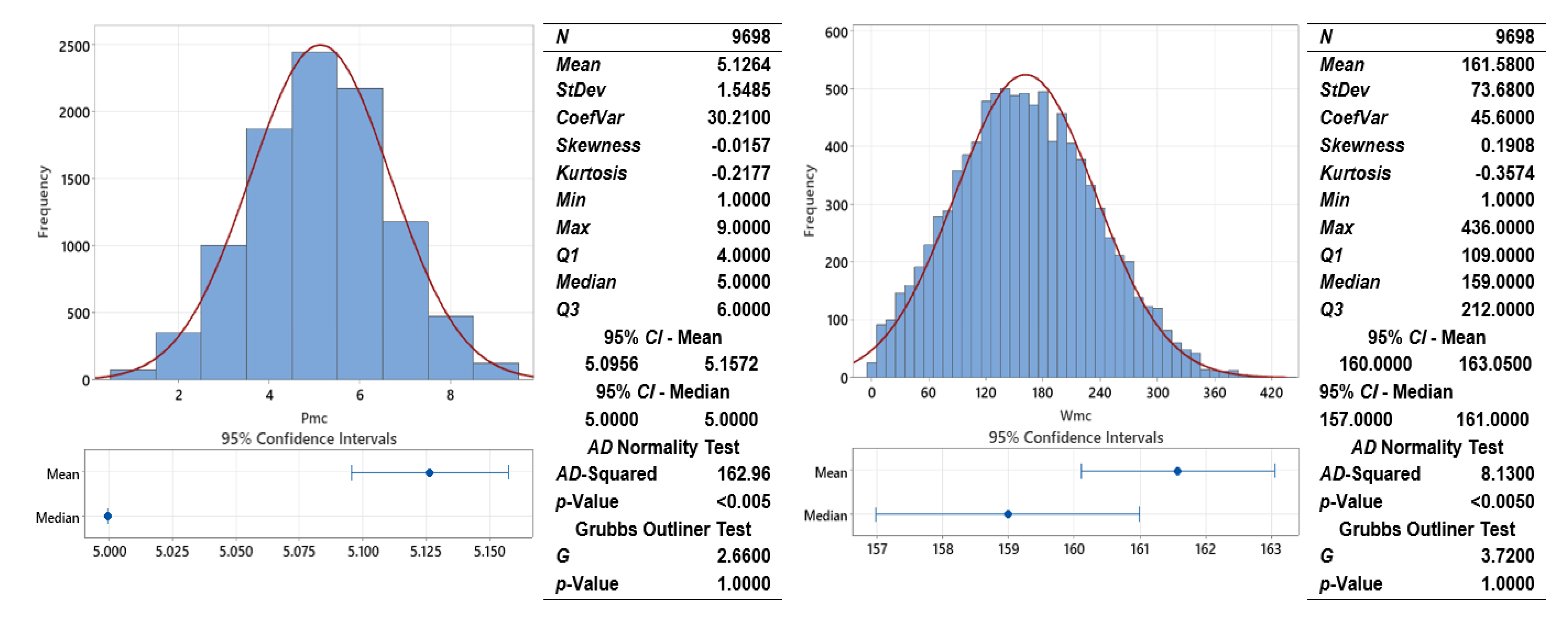
2.3. Monte Carlo Simulation Experiment

Monte Carlo simulation is used to generate a set of output (dependent) variables based on the distributions of input variable data, either known or estimated in advance, most of the time, to avoid performing a large number of experiments necessary to determine a mathematical model for assessing the output variable.
Monte Carlo simulation was conducted in this paper to improve the linear regression model of Ra. Due to many variations of input factors (P and W), it was assumed that the newly obtained MC regression model should be better at evaluating roughness Ra compared to the RaLM DOE model.
The coupling of input variables (P, W) with the output variable (Ra) necessary for performing the simulation was made based on Formula (2) for evaluating roughness RaLM using the obtained DOE model:
R aLM   =   f ( P a ,   W a )
The estimated roughness value R amcLM of the MC model for input variables P and W was obtained based on the Uniform distribution by a random selection of the X (P or W) input variable value between the lower limit (a) and the upper (b) limit. The parameters (a) and (b) are the continuous uniform distribution parameters (Figure 4).
For any value of the X in the interval a     x   1 <   x 2     b , the probability was calculated using the formula:
P a     X     b   =   x 2     x 1 ( b     a )
The uniform distribution parameters (a) and (b) for the variables P and W were determined based on their minimum and maximum values as follows:
(a)P = 3.0
(b)P = 7.0
(a)W = 52.0
(b)W = 270.0
The estimated number of iterations in the Monte Carlo simulation was 10,000.
After performing the Monte Carlo simulation, the multiple regression method was used to generate a statistical model to determine the influence of two or more independent quantitative factors X for the dependent variable Y. The method included the option of performing a stepwise regression where a subset of variables X with the greatest impact on the change in the value of the dependent variable Y was selected. Moreover, the impact was also identified by the ANOVA test. The expected outcome was the response surface equation model for the surface roughness prediction model RamcLM. To determine the efficiency of the model, the following parameters were determined: R2, R2(adj), Test data R2, and correlation coefficient RamcLM vs. Ramc. The response surface (Pamc, Wmc) vs. RamcLM. was represented graphically.

2.4. Multiple Sample Comparison Test of Roughness

This paper suggests the use of the Multiple Sample Comparison Test to compare the sample values of two or more independent variables (factors). In this case, factors were represented by the following roughness values: Rao, RaoLM, Ra, RaLM, Ramc, and RamcLM. The testing was carried out to establish the existence of significant differences between the means of populations from which the samples had been drawn. In addition, this paper intended to ascertain whether there was a significant difference between the linear models (RaLM, RamcLM) of roughness obtained from DOE and Monte Carlo experiments and the roughness model (RaoLM) obtained as a result of the preliminary experiment for intuitively selected values of process parameters P and W. The testing of uniformity (homogeneity) and the comparison of samples were done by testing the mean values of factors using ANOVA under the hypothesis that all samples had the same mean value. All the equations necessary for the multiple sample comparison test and their meanings are given in Figure S1.
Furthermore, Tukey’s pairwise comparison tests (multiple range tests) were suggested to detect the means of those factors that differed significantly from others. To visually display the ANOVA results the following graphic representations were employed: Tukey’s Difference of Means, Interval plot, Individual plot, and Box-and-Whisker plot.

2.5. Optimization of Process Parameters

Surface texturing is an industrial process whereby certain roughness required by the client needs to be achieved in a given interval or with desired default values. Automatically, the manufacturer is required to identify and optimize the parameters of the production process to minimize unacceptable losses, that is, rejects. Given the request, the ultimate objective of this study was to determine optimal values of P and W parameters to achieve the desired surface roughness. As shown in Figure 1, two types of process parameters optimization method were foreseen:
  • Determination of optimal P and W interval values based on the default Ra interval.
  • Determination of optimal P and W interval values based on the desired default Ra value.
As the key performance indicator of optimization, the process capability ratio (Cpk) was suggested and calculated using the Formulas under (4)–(6) [38].
C pk = min C pu ,   C pl
C pu = USL     μ 3 σ
C pl = μ     LSL 3 σ
where:
Cpk—Process capability ratio
Cpu—Process capability Upper specification limit (USL)
Cpl—Process capability Lower specification limit (LSL)
µ—Sample mean
σ—Sample standard deviation
The once-established Cpk represented a deviation from the optimized average surface roughness (Ra) and previously defined upper and lower specification limits (LSL/USL) for surface roughness. The benchmark was Cpk > 1.33. The greater the Cpk, the greater the likelihood that during the surface texturing of the sample, the values of Ra would remain within the default LSL/USL limits for parameters P and W.

3. Results and Discussion

3.1. Preliminary Experiment

The descriptive statistics results of the preliminary experiment for factors (Po, Wo) and the response variable Rao are shown in Figure 5, Figure 6 and Figure 7. A total of 27 experiments were performed to determine the surface roughness Rao for the intuitively determined values of Po and Wo factors. Considering that experiments were conducted at only three levels (3, 5, 7), the Po factor had a high variation coefficient CoefVar = 33.28%, whereas the Wo factor had a mean coefficient of variation CoefVar = 19.54%. Based on Q3, 75% of Po data was below 7 passes, and the Wo was in 75% of cases lower than 128 mW. Based on the skewness indicator, Po had a symmetric distribution, whereas Wo had a positive or right-skewed distribution. According to the AD Normality Test, neither factor had a normal distribution of data (p-Value < 0.005). Furthermore, according to the Grubbs’ outlier test, no outlier was found.
As shown in Figure 6, the response variable (Rao) had an extremely high coefficient of variation (CoefVar = 91.27%), and this was probably due to a variation in factor values. The probability plot showed a huge waste of data, as almost all response variable values were outside the confidence interval lines and the mean line. It should be observed that most values (75%) of Rao were less than 0.0820, whereas the maximum value was 0.2720. Based on the author’s experience, the lower roughness is the better to make the forming of wear-resistant layers more effective. It can be observed that, according to intuitively set factor values, the experiment generated significantly lower values of Ra concerning the maximum values obtained for particular combinations of factors. The response variable Ra did not have a normal distribution nor an outlier. The interaction plot in Figure 6 shows the effect of changing one factor and the response variable against the constant value of the other factor. Given that the interactive lines were not parallel, we concluded that there was an interaction between Wo and Rao and a relationship between them and the value of Po.
Given the interaction between the factors Po and Wo and the Rao, the stepwise regression was performed to obtain a linear model of RaoLM = f (Po, Wo) as well as the variance analysis to examine by means of p-values the relevance of the influence of Po and Wo factors on the response variable value (Rao). The obtained regression model is represented by Equation (7):
R aoLM =   - 0.3541   +   0.01480 P 0   +   0.002041 W 0
To obtain the regression model, 30% of data were omitted and the Forward Stepwise Selection procedure was applied by gradually introducing input variables in the model provided that they remained in the model if they had a significant effect on the response variable. From the analysis of variance, given that the p-values were relatively low compared to the standard value of 0.05, both variables, that is, factors, had a significant effect on the response variable (Rao). The performance of the regression model R2 = 40.53%, R2(adj) = 33.09%, test data R2 = 60.10%, and correlation RaoRaoLM = 69.60% was relatively low. As a result, the obtained RaoLM model had a low possibility of prediction of Rao depending upon the changes in Ro and Wo. According to the response surface plot, it can generally be concluded that higher values of Rao were obtained with fewer passes Po and lower power rates.

3.2. DOE Experiment

A 2-factor interaction DOE experiment with a total of 14 coefficients was performed. For the experiment, 1 response variable (Ra) and 2 experimental factors (P and W) were determined. Using the previously suggested experiment structure, a total of 36 experiments were performed. The results of the descriptive statistics of factors are shown in Figure 8. The values of the P and W factors were randomly selected from the interval [3…7] and the interval [52…270], respectively. According to the Q1 parameter for P, 25% of the value was below 3 passes, whereas according to Q3, 75% of the value was below 7 passes. For the W factor, according to the parameter Q1, 25% of the value was below 101.50 mW, whereas according to Q3, 75% of the value was below 207.0 mW. The AD normality test showed that none of the factors had a normal distribution of data (p-Value = 0), nor the outlier values according to the Grubbs’ outlier test (p-value = 1). Given the skewness values, both factors had a relatively symmetrical distribution of data (however, not a normal distribution considering their p-values). Factor P had a negatively skewed or left-skewed distribution, whereas factor Wmc had a positively skewed or right-skewed distribution of data. The Kurtosis values for both factors were between −2 and +2, as expected for data with a normal distribution. The figure also shows 95% confidence intervals for the mean and median values, and it also shows that the mean and median values are relatively close.
Figure 9 shows the descriptive statistics results for the Ra variable. The Ra had a negatively skewed or left-skewed distribution of data, and the distribution of data followed a normal distribution as shown by the AD normality test p-value of 0.3380, which is rather high. The normal distribution of data of the response variable Ra could be also inferred from the probability plot of Ra. The distribution of the response variable was such that it showed no outlier value, as illustrated by the Grubbs’ outlier test (p-Value = 1). Figure 9 also shows the interaction plot. It shows a change between one of the factors and the response variable compared to the constant value of the other factor. Given that the interactive lines are not parallel, and two lines (P = 5 and P = 7) intersect, it can be concluded that there is a relationship between the factor W and roughness, and that Ra depends on the value of the factor P.
Figure 10 shows the results of the multiple regression analysis which was performed to obtain the surface roughness model RaLM = f (P, W) based on the results of the DOE experiment. To obtain the regression model, the fitting algorithm was used to perform the forward stepwise selection, starting from the model which included only the constant (Const.), by gradually adding one variable (factor) at a time, provided that after adding the variables they would be statistically significant (p-value = 0.00). The regression model RaLM was obtained in two steps, provided that only in the second step (Step 2), all three steps (Const., P, and W) were significant for the response variable as confirmed by the p-value = 0 for factors P and W. The obtained regression model is represented by Formula (8):
R aLM   =   0.0090   +   0.01034 P   +   0.000388 W
The significant effect of all three factors on RaLM was also confirmed by the variance analysis and by p-value = 0. In addition, the obtained values of R2 = 89.31, R2(adj) = 88.13, and the correlation coefficient RaRaLM = 92.40% are considerably higher than in the preliminary regression model RaoLM. The test data value of R2 = 70.40% was relevant which means that the RaLM mode had a good roughness prediction even for those P and W values that were left out from the model-making process by a stepwise regression fitting algorithm. From the total number of datasets, 30% of data were omitted from the regression model creation procedure. The importance of the DOE assessment of the experimental values of Ra with the new model RaLM is shown in the correlation Ra   -   RaLM C and surface RaLM plots.
Views of the surface roughness profile and SEM image following the laser texturing for three different laser powers (low, medium, and high laser power; 52 mW, 186 mW, and 270 mW) and passes (3, 5, and 7) are shown in Figure 11.
Figure 11 shows surface roughness profiles and SEM images of surfaces textured using three different laser powers (52 mW, 186 mW, and 270 mW) and irradiated using three different numbers of laser beam passes (3, 5, and 7). The representative profiles of each group of parameters (P and W) shown were randomly chosen because they approximately had the same profile, meaning that not the best, i.e., the most uniform profile within the given group had been chosen. The beams of 52 mW led to a decrease in surface roughness Ra (Ra = 0.016 ± 0.0031 μm) compared to the roughness of non-textured surfaces (Ra = 0.038 ± 0.0025 μm), as a lower laser beam power caused a smoother roughness profile. SEM images of the fs-laser textured samples using different laser beams powers show significant differences in the surface topography of samples processed using laser texturing with a laser power intensity of 52 mW compared to other intensities (186 mW and 270 mW). SEM images of samples subjected to texturing with an intensity of 52 mW show no changes in surface topography as compared to non-textured samples, as shown in Figure 9–52 mW. In other samples (subjected to laser texturing with laser beam intensities of 186 mW and 270 mW), ripple patterns in the ablated area as well as irregular laser deposition products such as microdroplets formed. The formation of loose microdroplets during the laser texturing process was the result of high peaks that arose on the roughness profiles at higher intensities and became more frequent as the number of laser beam passes increased. Micropores and microcracks contributed to the formation of deep grooves on the roughness profile. With the increase in power intensity of the laser beam (186 mW and 270 mW) and in the number of laser-beam passes, the intensity of the melting process increased (as a result, more microdroplets were generated). According to Pan et al. [39], the ablation that occurs at defined laser intensities occurs mainly due to spallation which is the result of the ejection of the surface layer of the material. As the melting and the formation of microdroplets on the sample surface at higher intensities increased (270 mW), it caused high surface roughness values Ra = 0.311 ± 0.0413 μm and expressed peaks on the roughness profile (Figure 11–250-7).

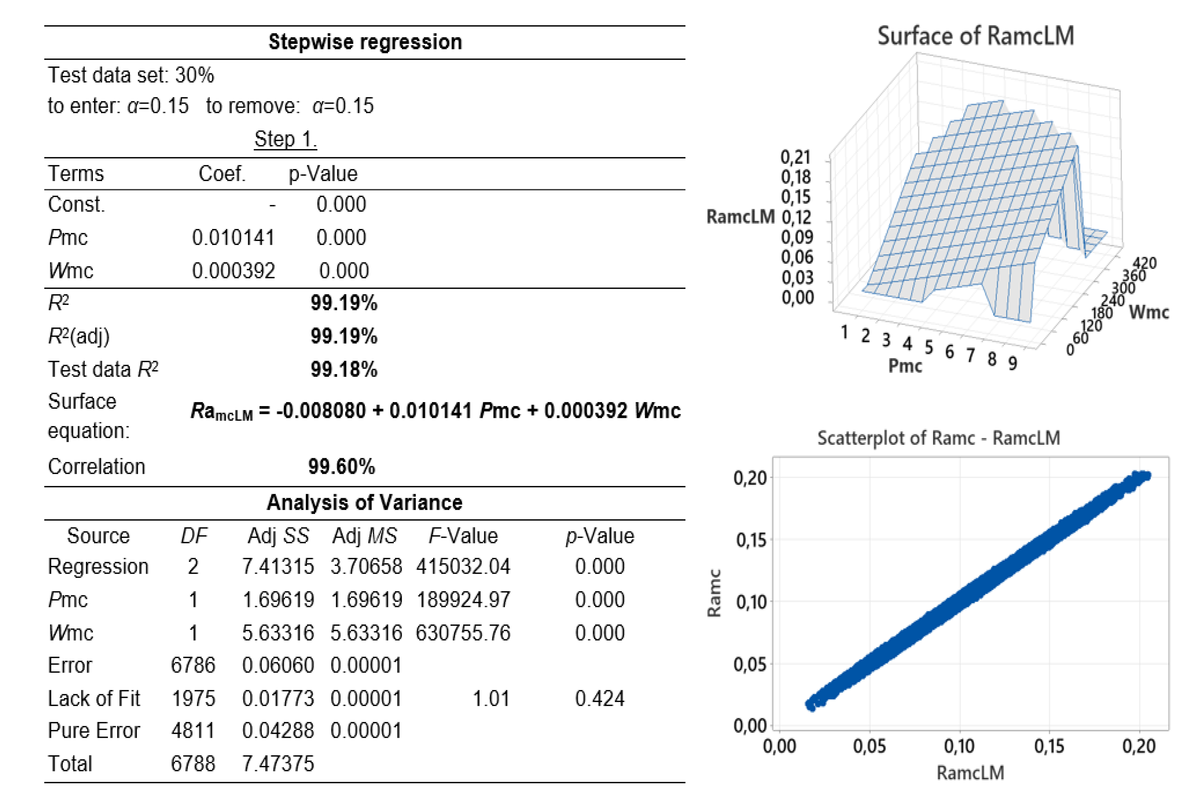
3.3. Monte Carlo Simulation Model

A Monte Carlo simulation was run with approximately 10,000 iterations. The assumed distribution of data for P and W was uniform within the interval of minimum and maximum factor values as indicated in the Section 2.3 Monte Carlo simulation experiment. The coupling of input factors (Pmc, Wmc) with the response variable (Ra) are connected by using Equation (8). The descriptive statistics results are shown in Figure 12 and Figure 13. The AD normality test results for factors Pmc and Wmc show that the distribution of data was not normal because the p-value was <0.005. The Grubbs’ outlier test shows that there were no outliers among the factors (p-value = 1.00). According to the Q1 parameter for factor Pmc, 25% of the value was below 4 passes, and 75% of the value was above 4 passes. According to the Q3 parameter, 75% of the value was below 6 passes, and 25% of the value was above 6 passes. Given the skewness values, both factors had a relatively symmetrical distribution of data (however, not a normal distribution considering their p-values). Pmc had a negatively skewed or left-skewed distribution, and Wmc had a positively skewed or right-skewed distribution. The Kurtosis values for both factors were between −2 and +2 as expected for data with a normal distribution. The figure also shows 95% confidence intervals for the mean and median values.
Figure 13 shows the descriptive statistics results of the Monte Carlo simulation for the response variable Ramc. Considering the foregoing considerations of the descriptive statistics parameters, Ramc had a positively or right-skewed distribution, which means that the distribution of data did not follow a normal distribution. The p-value of the AD normality test, which was <0.005, showed the same. In addition, the distribution of data for Ramc showed no outliers. For subsequent interval optimization of parameters of surface texturing, the consideration of the values of statistical parameters (Min, Max, Q1, and Q3) was of particular importance. The minimum value was 0.0139 mW, and the maximum value was 0.2028 mW. It is logical that the lower the value of roughness for the given P and W, the better, and according to Q3, only 25% of data for Ramc had a value higher than 0.1302 mW. The intervals of input process parameters (P and W) established by optimization gave the lowest value of Ramc.
As stated above, following the Monte Carlo simulation, the multiple regression procedure was performed to obtain a surface roughness prediction model R amcLM = f ( P , W ). As the model fitting procedure, forward stepwise selection was applied, starting with a model containing only a constant, and then adding variables (factors) to the model, provided that once they were added the variables became statistically significant ( p -value = 0.00). The forward stepwise algorithm made it possible to remove variables from or add them to the analysis in one of the following steps if they were no longer statistically relevant (p-value > 0.05). The results of the Monte Carlo regression model are shown in Figure 14. For removing, that is, for adding the variables to the model, the threshold of α   =   0.15 was used. As much as 30% of the total number of datasets was used to test the model during the performance of the forward stepwise procedure. In this case, already in the first step (Step 1) for all the three factors (Const. Pmc, Wmc), the significant effect of the p-value was determined along with the surface equation RamcLM (9).
R amcLM = 0.008080 + 0.010141 P mc + 0.000392 W mc
The significant effect of all three factors on RamcLM was confirmed by the analysis of variance (p-value = 0). Furthermore, it can be observed that the values of R2 = 99.19 and R2(adj) = 99.19 were significantly higher than in the DOE regression model RaLM, which justified the performance of the Monte Carlo simulation following the DOE experiment. The value of the test data R2 = 99.18% is of particular importance, which means that the RamcLM model had a good roughness prediction even for those P and W values which had been omitted from the process of model creation using the stepwise regression fitting algorithm. Typically, the value of the test data for R2 was lower than R2 obtained on training dataset, because the data from the test dataset were not included in the procedure of “learning” the RamcLM model. The robustness of the RamcLM model was also confirmed by a high correlation coefficient RamcLM vs. Ramc = 99.60% as can be seen from the scatterplot in Figure 14.

3.4. Multiple Sample Comparison of Roughness

As can be seen from the multiple comparisons of roughness test in Figure 15, the ANOVA table shows the results of the comparison of means between the groups of factors (row factor) and within the factors themselves (row error). The F-value, which in this case amounted to 10.52, was the ratio obtained by making an intra- and an inter-group assessment. Given that the p-value of the F-test was lower than 0.05, we conclude that the null hypothesis was not true and that there was a significant difference between the means of the indicated factors at a significance level of 5%. As Tukey’s pairwise comparison test at 95% confidence level shows, there was no significant difference in means between the roughness obtained using the DOE experiment and the roughness obtained using the Monte Carlo simulation and the respective LM models (Group A). In addition, there was no significant difference between the preliminarily obtained roughness and the respective LM model (Group B). Tukey’s mean difference plot shows that by two-pairs comparison, all factors in Group A differ from those in Group B. Such a difference in the results of the comparison was expected considering that the values of P and W in the preliminary experiment were intuitively, not randomly selected.

3.5. Optimization of Process Parameters

The optimization intervals of input parameters P and W and the response variable Ra were determined based on the surface and contour plots of Ra as shown in Figure 16. The contour plot shows that higher roughness values were obtained in the Ra = [0.1, 0.15], P = [4,7] and W = [160,270] intervals, and lower in the Ra = [0.05, 0.100], P = [3,4] and W = [52,126] intervals.
In light of the above considerations, final optimization intervals were suggested: Ra = [0.06, 0.09], P = [3,4], W = [52,126]. Figure 17 shows the Monte Carlo simulation results (1000 iterations) for the Ra interval (Ra = 0.06, 0.09) and the non-optimized values of the process parameters (P and W). The Cpk is 0.4957, which is certainly lower than the acceptable value (1.33). In the case of a new experiment, for interval values P = [3,4], W = [52,126], we would have a waste of Ra outside the interval of 31.69%, which is unacceptable.
From the total of 10,000 samples, 1574 samples were below the LSL limit, and 3595 were above the USL limit. Following the Monte Carlo simulation of the non-optimized intervals of process parameters, the first type of parameter interval optimization was performed to obtain the highest possible Cpk and the lowest percentage of samples outside the intervals.
After consecutive optimization iterations where the values of P and W changed, and after conducting the sensitivity analysis where the standard deviations for P and W (−50% do + 50%) were changed, the results for optimized intervals of process parameters P and W for the predefined Ra interval (Ra = [0.06, 0.09]) are shown in Figure 18.
This optimization contributed to achieving a satisfactory value for Cpk (Cpk = 1.5 > 1.33), whereas for the samples out of limits, the value was 0.00%. In the case of a new experiment, the number of passes and intervals P = [3,4] as well as the intensity W = [105,132] would have to be selected. The application of P and W values from the indicated intervals during the experiment would in 95% of cases ensure Ra values within the LSL = 0.06 and USL = 0.09 intervals. The table in Figure 18 shows that the mean = 0.0749, min = 0.0646, and max = 0.0853 values practically correspond to the optimization area of Ra in Figure 16. The second type of optimization is even more important for practical application than the previous one because a certain surface roughness (Ra) of the sample is normally required in practice. Additionally in this case, the obtained process parameters of P and W guaranteed, with a statistical certainty of 95%, that the default Ra would be obtained. Given that a real production process is involved here, achieving the exact default Ra is not possible, but rather a value within the LSL and USL interval range. Figure 19 shows the simulation results for the default RamcLM = 0.08. This latter was chosen because it is in the middle of the predefined interval for Ra as can be seen from the contour plot in Figure 16. In the case of a new experiment, the default value for RamcLM = 0.08 would be achieved if we conducted the experiment with the following intervals of P = [4,4] and W = [111,138]. Moreover, the satisfactory value of Cpk = 1.36 > 1.33 was obtained, whereas the performance capability for the samples out of limits was 0.00%.

4. Conclusions

This study investigates the influence of process parameters (number of passes P and power W) on the average surface roughness values (Ra) of Ti alloys by applying the femtosecond laser texturing technology. The optimization of the P and W process parameters was carried out. To determine the effect of the P and W parameters on Ra, before optimizing the process parameters, three experiments were carried out: a preliminary experiment, a DOE experiment, and a Monte Carlo simulation experiment. Based on these experiments, dependency models of Ra = f (P, W) were generated, and the values of Ra generated by each model were compared. In addition, the preliminary experiment was used to measure the roughness value range Ra = 0.038 ± 0.0025 μm on the untreated sample and the surface was analyzed using SEM. Subsequently, 27 Ti-alloy samples were textured using a femtosecond laser with intuitively chosen process parameters (Po = [3,5,7], Wo = [80,100,128]).
The texturing process was repeated three times for each value of the Po interval with each value of the Wo interval. The descriptive analysis results show a significant variation of roughness (Rao = 91.27%). The AD test shows that the distribution of Rao is not normal. The ANOVA test shows that a change in the Po and Wo parameters significantly affects the change of Rao. The fitting performance of the generated regression model RaoLM (7), R2 = 40.53%, R2(adj) = 33.09%, test data R2 = 60.10%, and correlation RaoRaoLM = 69.60 is relatively low. The preliminary model of RaoLM has a weak prediction performance of Ra. A 2-factor interactions DOE experiment showed a better result. A variation in roughness (Ra) of 39.11% is acceptable and the Ra values have a normal distribution as shown by the AD test (p = 0.3380). The fitting performance of the generated DOE regression model of RaLM (8) is significantly better compared to the preliminary model of RaoLM and is as follows: R2 = 89.31%, R2(adj) = 88.13%, test data R2 = 70.40%, and correlation RaRaLM = 92.40%. The analysis of the roughness values obtained by the DOE shows that the samples textured at lower laser beam power values (e.g., 52 mW) show lower values of parameters (Ra = 0.016 ± 0.0031 μm), even in relation to the non-textured sample (Ra) = 0.038 ± 0.0025 μm.
SEM images of the surface topography of samples for other (higher) laser beam power values show changes in the Ti-alloy surface in the form of ripple patterns, and irregular laser deposition products such as microdroplets. Microdroplets cause changes in the roughness profile in the form of peaks which result in higher values of roughness (Ra = 0.311 ± 0.0413 μm for the sample 270-7).
The objective of the third experiment using MC simulation was to generate a more accurate roughness prediction model compared to the DOE RaLM model. The objective was accomplished. The uniform distribution of data with a and b parameters (Pmc(3, 7), Wmc(52, 270)) was suggested. A total of 10,000 simulation iterations were performed and the coupling function was RaLM. The fitting performance of the generated MC regression model of RamcLM (9) was better compared to the DOE RaLM model and, generally, the values were much higher: R2 = 99.19%, R2(adj) = 99.19%, test data R2 = 99.18%, and correlation RaRaLM = 99.60%. Multiple sample comparison test of roughness (Figure 15) shows no difference in means between the DOE and MC models and displays uniformity of data values as indicated by Tukey’s pairwise comparison plot. It could therefore be concluded that the MC regression model will provide reliable predictions of roughness for any new combination of process parameters given a high value of Test data R2. It can be concluded from Tukey’s difference of means plot (Figure 15) that there is a significant difference in means between the DOE RaLM and the MC RamcLM models in respect of the preliminary RaoLM model. The optimization of process parameters was done based on the RamcLM model and with regard to the method of defining the surface roughness default value. In the first method, the default surface roughness was given within the interval RamcLM = [0.06, 0.09]. The optimized intervals of process parameters that contribute to achieving such an interval were: P = [3,4] and W = [105,132]. In the second method, the default surface roughness was RamcLM = 0.08, and the optimized intervals of process parameters needed to achieve such an interval were P = [4,4] and W = [111,138].
For future research, we suggest optimizing the surface roughness of Ti alloys to achieve the highest wear resistance of the applied layer.

Supplementary Materials

The following supporting information can be downloaded at: https://www.mdpi.com/article/10.3390/coatings13071180/s1. Figure S1. ANOVA sample comparison test of roughness.

Author Contributions

D.L.: conceptualization, methodology, software, visualization, writing; S.J.: investigation, resources, conceptualization, writing; H.S.: validation. All authors have read and agreed to the published version of the manuscript.

Funding

This research was funded by the European Regional Development Fund, grant number KK.01.1.1.07.0031.

Institutional Review Board Statement

Not applicable.

Informed Consent Statement

Not applicable.

Data Availability Statement

Not applicable.

Conflicts of Interest

The authors declare no conflict of interest.

References

  1. Holmberg, K.; Erdemir, A. Influence of tribology on global energy consumption, costs and emissions. Friction 2017, 5, 263–284. [Google Scholar] [CrossRef] [Green Version]
  2. Basiaga, M.; Walke, W.; Paszenda, Z.; Kajzer, A. The effect of EO and steam sterilization on the mechanical and electrochemical properties of titanium Grade 4. Mater. Technol. 2016, 50, 149–154. [Google Scholar] [CrossRef]
  3. Jin, Z.M.; Zheng, J.; Li, W.; Zhou, Z.R. Tribology of medical devices. Biosurface Biotribol. 2016, 2, 173–192. [Google Scholar] [CrossRef]
  4. Dai, F.; Zhang, Z.; Ren, X.; Lu, J.; Huang, S. Effects of laser shock peening with contacting foil on micro laser texturing surface of Ti6Al4V. Opt. Lasers Eng. 2018, 101, 99–105. [Google Scholar] [CrossRef]
  5. Temmler, A.; Liu, D.M.; Drinck, S.; Luo, J.B.; Poprawe, R. Experimental investigation on a new hybrid laser process for surface structuring by vapor pressure on Ti6Al4V. J. Mater. Process. Technol. 2020, 277, 116450. [Google Scholar] [CrossRef]
  6. Chérif, M.; Loumena, C.; Jumel, J.; Kling, R. Performance of Laser Surface Preparation of Ti6Al4 V. Procedia CIRP 2016, 45, 311–314. [Google Scholar] [CrossRef] [Green Version]
  7. Grabowski, A.; Sozańska, M.; Adamiak, M.; Kępińska, M.; Florian, T. Laser surface texturing of Ti6Al4V alloy, stainless steel and aluminium silicon alloy. Appl. Surf. Sci. 2018, 461, 117–123. [Google Scholar] [CrossRef]
  8. Martínez, J.M.; Gomez, J.S.; Ares, P.F.M.; Fernandez Vidal, S.R.; Batista Ponce, M. Effects of Laser Microtexturing on the Wetting Behavior of Ti6Al4V Alloy. Coatings 2018, 8, 145. [Google Scholar] [CrossRef] [Green Version]
  9. Ahuir-Torres, J.I.; Arenas, M.A.; Perrie, W.; de Damborenea, J. Influence of laser parameters in surface texturing of Ti6Al4V and AA2024-T3 alloys. Opt. Lasers Eng. 2018, 103, 100–109. [Google Scholar] [CrossRef]
  10. Zhou, J.; Sun, Y.; Huang, S.; Sheng, J.; Li, J.; Agyenim-Boateng, E. Effect of laser peening on friction and wear behavior of medical Ti6Al4V alloy. Opt. Laser Technol. 2019, 109, 263–269. [Google Scholar] [CrossRef]
  11. Zhang, L.C.; Chen, L.Y.; Wang, L. Surface Modification of Titanium and Titanium Alloys: Technologies, Developments, and Future Interests. Adv. Eng. Mater. 2020, 22, 1901258. [Google Scholar] [CrossRef]
  12. Moura, C.G.; Carvalho, O.; Gonçalves, L.M.V.; Cerqueira, M.F.; Nascimento, R.; Silva, F. Laser surface texturing of Ti-6Al-4V by nanosecond laser: Surface characterization. Ti-oxide layer analysis and its electrical insulation performance. Mater. Sci. Eng. C 2019, 104, 109901. [Google Scholar] [CrossRef]
  13. Zaifuddin, A.; Aiman, M.; Quazi, M.; Ishak, M.; Shamini, J. Influence of Laser Surface Texturing (LST) Parameters on the Surface Characteristics of Ti6Al4V and the Effects Thereof on Laser Heating. Lasers Eng. 2021, 51, 355–367. [Google Scholar]
  14. Vázquez Martínez, J.M.; Salguero Gómez, J.; Batista Ponce, M.; Botana Pedemonte, F.J. Effects of Laser Processing Parameters on Texturized Layer Development and Surface Features of Ti6Al4V Alloy Samples. Coatings 2018, 8, 6. [Google Scholar] [CrossRef] [Green Version]
  15. Pfleging, W.; Kumari, R.; Besser, H.; Scharnweber, T.; Majumdar, J.D. Laser surface textured titanium alloy (Ti–6Al–4V): Part 1—Surface characterization. Appl. Surf. Sci. 2015, 355, 104–111. [Google Scholar] [CrossRef]
  16. Rajan, S.S.; Manivasagam, G.; Ranganathan, M.; Swaroop, S. Influence of laser peening without coating on microstructure and fatigue limit of Ti-15V-3Al-3Cr-3Sn. Opt. Laser Technol. 2019, 111, 481–488. [Google Scholar] [CrossRef]
  17. Kumari, R.; Scharnweber, T.; Pfleging, W.; Besser, H.; Majumdar, J.D. Laser surface textured titanium alloy (Ti–6Al–4V)—Part II—Studies on bio-compatibility. Appl. Surf. Sci. 2015, 357, 750–758. [Google Scholar] [CrossRef]
  18. Wang, Z.; Song, J.; Wang, T.; Wang, H.; Wang, Q. Laser Texturing for Superwetting Titanium Alloy and Investigation of Its Erosion Resistance. Coatings 2021, 11, 1547. [Google Scholar] [CrossRef]
  19. Xu, Y.; Li, Z.; Zhang, G.; Wang, G.; Zeng, Z.; Wang, C.; Wang, C.; Zhao, S.; Zhang, Y.; Ren, T. Electrochemical corrosion and anisotropic tribological properties of bioinspired hierarchical morphologies on Ti-6Al-4V fabricated by laser texturing. Tribol. Int. 2019, 134, 352–364. [Google Scholar] [CrossRef]
  20. Ma, Z.; Song, J.; Fan, H.; Hu, T.; Hu, L. Preparation and Study on Fretting Tribological Behavior of Composite Lubrication Structure on the Titanium Alloy Surface. Coatings 2022, 12, 332. [Google Scholar] [CrossRef]
  21. Yang, C.; Mei, X.; Tian, Y.; Zhang, D.; Li, Y.; Liu, X. Modification of wettability property of titanium by laser texturing. Int. J. Adv. Manuf. Technol. 2016, 87, 1663–1670. [Google Scholar] [CrossRef] [Green Version]
  22. Kubiak, K.J.; Wilson, M.C.T.; Mathia, T.G.; Carval, P. Wettability versus roughness of engineering surfaces. Wear 2011, 271, 523–528. [Google Scholar] [CrossRef] [Green Version]
  23. Salguero, J.; Del Sol, I.; Vazquez-Martinez, J.M.; Schertzer, M.J.; Iglesias, P. Effect of laser parameters on the tribological behavior of Ti6Al4V titanium microtextures under lubricated conditions. Wear 2019, 426–427, 1272–1279. [Google Scholar] [CrossRef]
  24. Maalouf, M.; Abou Khalil, A.; Di Maio, Y.; Papa, S.; Sedao, X.; Dalix, E.; Peyroche, S.; Guignandon, A.; Dumas, V. Polarization of Femtosecond Laser for Titanium Alloy Nanopatterning Influences Osteoblastic Differentiation. Nanomaterials 2022, 12, 1619. [Google Scholar] [CrossRef] [PubMed]
  25. Kumar, D.; Nadeem Akhtar, S.; Kumar Patel, A.; Ramkumar, J.; Balani, K. Tribological performance of laser peened Ti–6Al–4V. Wear 2015, 322–323, 203–217. [Google Scholar] [CrossRef]
  26. Kümmel, D.; Hamann-Schroer, M.; Hetzner, H.; Schneider, J. Tribological behavior of nanosecond-laser surface textured Ti6Al4V. Wear 2019, 422–423, 261–268. [Google Scholar] [CrossRef] [Green Version]
  27. Bai, H.; Zhong, L.; Kang, L.; Liu, J.; Zhuang, W.; Lv, Z.; Xu, Y. A review on wear-resistant coating with high hardness and high toughness on the surface of titanium alloy. J. Alloys Compd. 2021, 882, 160645. [Google Scholar] [CrossRef]
  28. Bonse, J.; Krüger, J.; Höhm, S.; Rosenfeld, A. Femtosecond laser-induced periodic surface structures. J. Laser Appl. 2012, 24, 042006. [Google Scholar] [CrossRef]
  29. Rajab, F.H.; Liauw, C.; Benson, P.; Li, L.; Whitehead, K. Production of hybrid macro/micro/nano surface structures on Ti6Al4V surfaces by picosecond laser surface texturing and their antifouling characteristics. Colloids Surf. B Biointerfaces 2017, 160, 688–696. [Google Scholar] [CrossRef] [Green Version]
  30. Bhaduri, D.; Batal, A.; Dimov, S.; Zhang, Z.; Dong, H.; Fallqvist, M.; M’Saoubi, R. On Design and Tribological Behaviour of Laser Textured Surfaces. Procedia CIRP 2017, 60, 20–25. [Google Scholar] [CrossRef]
  31. Dumas, V.; Rattner, A.; Vico, L.; Audouard, E.; Dumas, J.C.; Naisson, P.; Bertrand, P. Multiscale grooved titanium processed with femtosecond laser influences mesenchymal stem cell morphology, adhesion, and matrix organization. J. Biomed. Mater. Res. A 2021, 100, 3108–3116. [Google Scholar] [CrossRef]
  32. Kuczyńska, D.; Kwaśniak, P.; Pisarek, M.; Borowicz, P.; Garbacz, H. Influence of surface pattern on the biological properties of Ti grade 2. Mater. Charact. 2018, 135, 337–347. [Google Scholar] [CrossRef]
  33. Schnell, G.; Staehlke, S.; Duenow, U.; Nebe, B.; Seitz, H. Femtosecond Laser Nano/Micro Textured Ti6Al4V Surfaces—Effect on Wetting and MG-63 Cell Adhesion. Materials 2019, 12, 2210. [Google Scholar] [CrossRef] [Green Version]
  34. Bonse, J.; Kirner, S.V.; Griepentrog, M.; Spaltmann, D.; Krüger, J. Femtosecond Laser Texturing of Surfaces for Tribological Applications. Materials 2018, 11, 801. [Google Scholar] [CrossRef] [Green Version]
  35. Li, B.; Li, H.; Huang, L.; Ren, N.; Kong, X. Femtosecond pulsed laser textured titanium surfaces with stable superhydrophilicity and superhydrophobicity. Appl. Surf. Sci. 2016, 389, 585–593. [Google Scholar] [CrossRef]
  36. Jalil, S.A.; Akram, M.; Bhat, J.A.; Hayes, J.J.; Singh, S.C.; El Kabbash, M.; Guo, C. Creating superhydrophobic and antibacterial surfaces on gold by femtosecond laser pulses. Appl. Surf. Sci. 2020, 506, 144952. [Google Scholar] [CrossRef]
  37. Romano, J.M.; Garcia-Giron, A.; Penchev, P.; Dimov, S. Triangular laser-induced submicron textures for functionalising stainless steel surfaces. Appl. Surf. Sci. 2018, 440, 162–169. [Google Scholar] [CrossRef] [Green Version]
  38. Montgomery, D.C. Introduction to Statistical Quality Control; John Wiley & Sons: Hoboken, NJ, USA, 2013. [Google Scholar]
  39. Pan, X.; He, W.; Cai, Z.; Wang, X.; Liu, P.; Luo, S.; Zhou, L. Investigations on femtosecond laser-induced surface modification and periodic micropatterning with anti-friction properties on Ti6Al4V titanium alloy. Chin. J. Aeronaut. 2022, 35, 521–537. [Google Scholar] [CrossRef]
Figure 1. Overview of research steps and methods.
Coatings 13 01180 g001
Figure 2. Pictorial representation of surface roughness; Ra Rz and Rmax.
Coatings 13 01180 g002
Figure 3. (a) The roughness profile and (b) SEM image of reference sample RS.
Coatings 13 01180 g003
Figure 4. Uniform distribution.
Coatings 13 01180 g004
Figure 5. Descriptive statistics of the preliminary experiment for Po and Wo.
Coatings 13 01180 g005
Figure 6. Descriptive statistics of the preliminary experiment for Rao.
Coatings 13 01180 g006
Figure 7. Analysis of preliminary regression model, RaoLM.
Coatings 13 01180 g007
Figure 8. Descriptive statistics of DOE experiment for P and W factors.
Coatings 13 01180 g008
Figure 9. Descriptive statistics of DOE experiment for Ra response variable.
Coatings 13 01180 g009
Figure 10. Analysis of DOE RaLM regression model.
Coatings 13 01180 g010
Figure 11. (a1,b1,c1) Surface topography and (a2,b2,c2) SEM images of samples S52, S186, S270.
Coatings 13 01180 g011aCoatings 13 01180 g011bCoatings 13 01180 g011c
Figure 12. Descriptive statistics of Monte Carlo simulation for Pmc and Wmc factors.
Coatings 13 01180 g012
Figure 13. Descriptive statistics of Monte Carlo simulation of Rmc response.
Coatings 13 01180 g013
Figure 14. Analysis of Monte Carlo regression model, RmcLM.
Coatings 13 01180 g014
Figure 15. Results of multiple sample comparison of roughness, Ra.
Coatings 13 01180 g015
Figure 16. Determination of process parameters optimization interval.
Coatings 13 01180 g016
Figure 17. Unoptimized intervals of process parameters P and W for predefined Ra interval.
Coatings 13 01180 g017
Figure 18. Optimized intervals of process parameters P and W for predefined Ra interval.
Coatings 13 01180 g018
Figure 19. Optimized intervals of process parameters P and W for predefined Ra value.
Coatings 13 01180 g019
Disclaimer/Publisher’s Note: The statements, opinions and data contained in all publications are solely those of the individual author(s) and contributor(s) and not of MDPI and/or the editor(s). MDPI and/or the editor(s) disclaim responsibility for any injury to people or property resulting from any ideas, methods, instructions or products referred to in the content.

