Compressive Strength Estimation of Waste Marble Powder Incorporated Concrete Using Regression Modelling

Abstract

A tremendous volumetric increase in waste marble powder as industrial waste has recently resulted in high environmental concerns of water, soil and air pollution. In this paper, we exploit the capabilities of machine learning to compressive strength prediction of concrete incorporating waste marble powder for future use. Experimentation has been carried out using different compositions of waste marble powder in concrete and varying water binder ratios of 0.35, 0.40 and 0.45 for the analysis. Effect of different dosages of superplasticizer has also been considered. In this paper, different regression algorithms to analyse the effect of waste marble powder on concrete, viz., multiple linear regression, K-nearest neighbour, support vector regression, decision tree, random forest, extra trees and gradient boosting, have been exploited and their efficacies have been compared using various statistical metrics. Experiments reveal random forest as the best model for compressive strength prediction with an R2 value of 0.926 and mean absolute error of 1.608. Further, shapley additive explanations and variance inflation factor analysis showcase the capabilities of the best achieved regression model in optimizing the use of marble powder as partial replacement of cement in concrete.

1. Introduction

Concrete is considered as the second most used material on earth, with cement comprising the primary source of its binder material. Cement production is the source of about 8% of the world’s carbon dioxide production. It is also the most expensive concrete component. This forces engineers to choose carefully between high strength and affordability. Numerous studies have been performed in order to introduce newer materials as a replacement for cement. However, the conventional approach of relying solely on laboratory test data is quite costly and inefficient. One requires impractically huge number of controlled testing to reach a reasonable conclusion and thus roll out innovations in the construction industry. In times of computing advancements, it becomes imperative to introduce newer technologies in concrete testing. Marble is another extensively used construction material, representing the most used natural stone in the world [1]. About 500 million metric tons of the material is mined annually [2] out of which, approximately 10% originates from India [3]. The Rajasthan state alone accounts for 85–90% of Indian marble production. The marble industry produces marble dust every year which bears essentially no utility, resulting in:

• Damage to soil due to dumping of waste;
• Degradation of groundwater

There is a lack of codal provisions to use marble dust in concrete. Consequently, this has prevented any large-scale commercial use. Well-documented research on the use of a certain amount of marble dust in concrete can significantly reduce costs. Its importance becomes quite evident given the losses that the industry has suffered from the COVID-19 pandemic, damage that will take several years to recover from. Cost reductions can help to bridge the gap. Further, large quantities of solid waste generated from the marble industry also need to be recycled to boost environment protection and economy.

With the advancement of various soft computing techniques, data handling capabilities of researchers have increased and are more efficient now over conventional ways. As a result, many algorithms have gained popularity in the due course of time. However, a detailed comparison between these algorithms still remains less explored and need further study. Use of machine learning (ML) algorithms can provide a reliable mix design for industry. In the long run, the Indian Standard codes can also be updated with marble dust parameters. ML is being increasingly used in civil engineering for the purpose of strength prediction. Elyas Asadi Shamsabadi et al. [4] studied marble-dust-incorporated concrete for strength predictions. Extreme Gradient Boosting (XGB) and ANN were found to be appropriate models, while XGB had fewer errors in prediction, on the other hand, Artificial Neural Network ANN was deemed to be more sensitive to marble dust content. The study also confirmed the non-pozzolanic nature of marble dust incorporated in concrete. Further, Karimipour et al. [5] conducted a soft-computing-based study involving marble dust in steel-fiber-reinforced self-consolidation concrete. In addition, other ingredients such as granite, red mud and limestone were also used. ANN, GMDH-NN and GMDH-Combi models were exploited to predict split tensile strength as well as compressive correction factors. It was observed that ANN using 4 neurons and 1 hidden layer gave better performance than other 2 models. Of the other two, GMDH-NN (neural networks group method of data handling) performed better than GMDH-Combi (combinatorial algorithm group method of data handling). Further, Hong-Hu Chu et al. [6] explored gene-expression programming (GEP) and multi-expression programming (MEP) to predict the compressive strength of geopolymer concrete. Various parameters such as curing regime, silica and superplasticizer content, curing period and age of the sample were related to compressive strength. However, GEP resulted in higher correlation coefficient, minimal statistical error and simplicity. In addition, it covered the impact of each independent parameter, as it was utilized for parametric study and sensitivity as well. Swaidani et al. [7] discussed the use of scoria as a partial replacement for cement in making environmentally friendly concrete. Concrete strength and durability were studied for the same purposes. It was inferred that ANN model was well suited for concrete strength prediction at different curing times for different mix ingredients. Further, it was also observed that compressive strength prediction for concrete comprising ground granulated blast furnace slag could also be achieved using ANN. A Multiple Regression Analysis (MRA) and an ANN model were constructed for comparing the predicted compressive strength of high-performance concrete using nano silica and copper slag as partial replacement and fine aggregate replacement, respectively, [8], by collecting data from laboratory experiments. Levenberg–Marquardt (LM) algorithm was used for generating the ANN model. Models for predicting compressive strength on 22 mixes were generated using MRA analysis and ANN, with ANN resulting in higher accuracy and correlation values. Further, Naddaf et al. [9] proposed an ANN and GEP model to train and study 640 different mix designs and predict various properties by partially replacing cement with nano silica and micro silica by weight. Kazemi et al. [9] presented an ANN model for compressive strength prediction of mortar mixes containing cement of different strengths. The study predicted good accuracy and higher R value in predicting the compressive strength of the mortar. Later, Naderpour et al. [10] exploited ANN to predict the compressive strength of environmentally friendly concrete, comprising recycled aggregate material. The data used for developing the ANN Model were prepared from the literature. Back propagation network was used in the study, resulting in efficient predictions. An Adaptive Neuro Fuzzy Inference System (ANFIS) model was provided by Nejadi et al. [11] that established a relationship between the compressive strength of self-compacting concrete (SCC) and slump flow and mix proportion. In past studies, SCC has proved advantageous in achieving sustainable characteristics, reduction in the overall structural costs, increase in construction rate, quality of casted structure and increase in construction productivity. Poon et al. [12] aimed to predict the compressive strength of concrete comprising recycled aggregate, using ANN. The model constituted 14 different properties of the constituents to predict the 28-day compressive strength of the concrete. Soft computing has been found to have applications in recycled concrete, where deep-learning-based techniques have been found to outperform traditional neural networks in terms of precision, generalization and efficiency [13]. A deep neural network was designed by Ly et al. [14] for predicting compressive strength of concrete with rubber content, resulting in high accuracy. Further, Nunez et al. [15] studied and analysed different ML models predicting the compressive strength of concrete. It was observed that ANN was the best-suited method for prediction, but was accompanied by a lack of clarity in the prediction process with high computational costs. Fuzzy-logic-based models had similar accuracy, but were of higher complexity. Furthermore, Support Vector Machine (SVM)-based models were considered to have lower computational costs than ANN but with comparable accuracy. Hybrid models were found to be the most promising due to the presence of a secondary model to obtain hyperparameters for the main model. Mansouri et al. [16] explored the usage of 4 types of soft computing techniques, viz., ANN, ANFIS, MARS (Multivariate Adaptive Regression Splines) and M5Tree (M5 Model Tree), to predict FRP-confined concrete. These models were found to outperform the existing models, with ANN resulting in the best estimation of strain enhancement ratio. Sahoo et al. [17] studied fly-ash-based concrete using ANN modelling by considering two different replacement levels, i.e., one at Low-25%, the other at High-40%. Fly ash concrete resulted in a better performance than control concrete over long periods of sulphate exposure. The ANN model was developed by minimization of mean square error. Furthermore, the R${}^2$ values ranged from 0.953 to 1.00, depicting high accuracy and reliability of the model. Recently, Khan et al. [18] discussed the performance of ANN, ANFIS and GEP models in order to estimate compressive strength of geopolymer concrete based on fly ash, with ANFIS giving the best performance of all.

As can be observed, there are only a handful of studies regarding the effects on compressive strength for partial replacement of cement by marble dust. Although a huge number of experimental studies have been carried out for investigating possible effects of waste marble powder (WMP) on concrete, there is still a lack of in-depth understanding on use of WMP in concrete. Regarding the use of soft computing, it remains in its infancy in civil engineering applications. As discussed above, soft computing has been largely applied in materials other than marble dust, such as fly ash, FRP and rubber, to name a few. This study aims to contribute by filling this gap and thus, pave the way for further research and eventual codification of marble dust in concrete. The soft computing approach makes use of various algorithms to arrive at its conclusions. There exists a relentless lack of a comprehensive understanding related to the dosage level of WMP so as to intensify the engineering properties of concrete. The WMP characteristics vary based on geological and weather conditions, and also on the methods for production of marble sheets for construction industries. In addition, thermogravimetric results along with various phases in cement paste containing WMP in cement and concrete exhibited the benign nature of the product [19,20]. Various alterations in experimentation make it difficult to generalise and hence, achieve a standard mixture design for WMP-incorporated concrete. Exploiting ML techniques can help in achieving cost- and time-effective simulation of the same, thus maximising the application of WMP in concrete industry by complementing the outcomes acquired from the already existing experimental investigations.

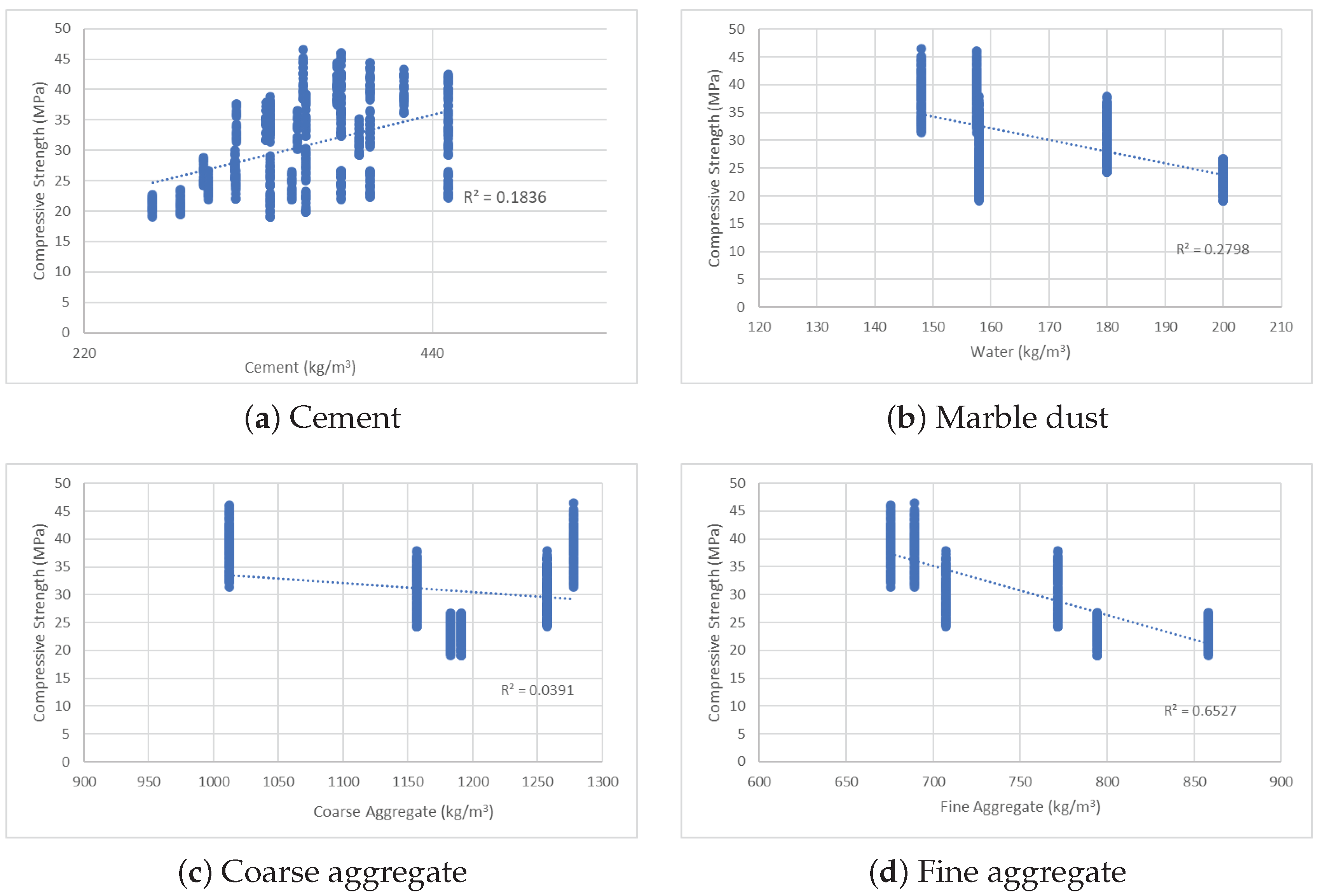
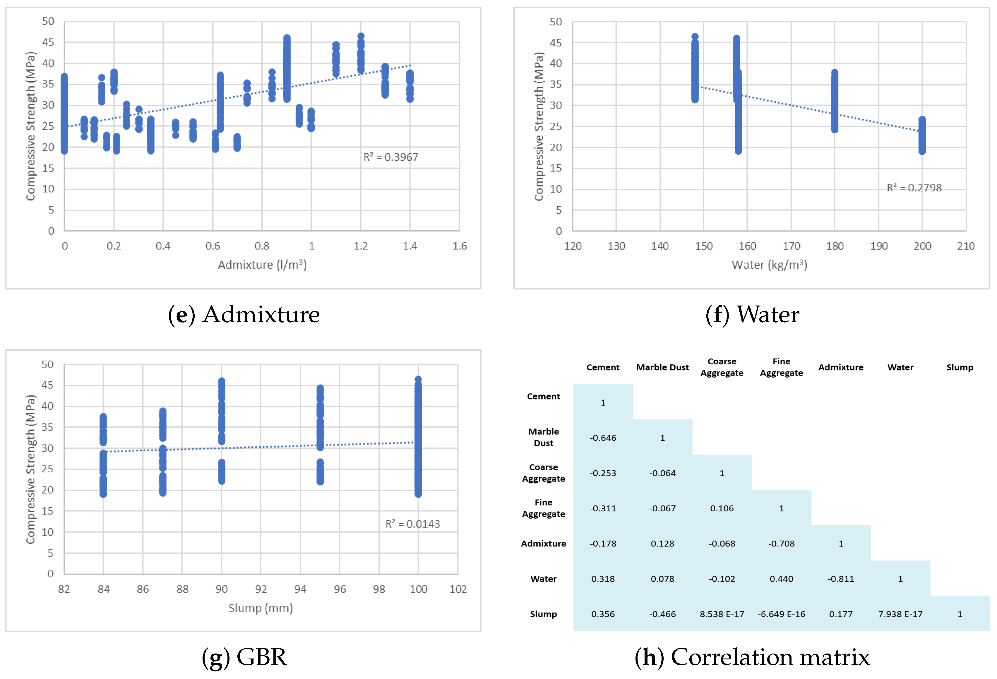
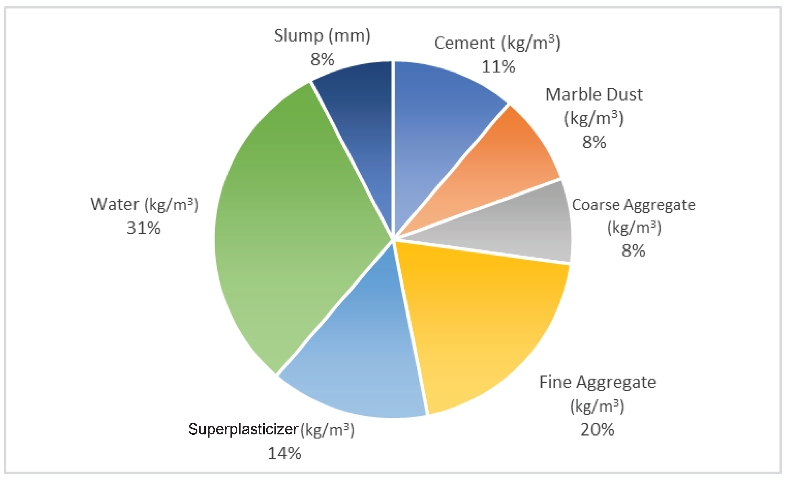
2. Data Collection and Modelling

Data for the present study were collected from experimental trials previously conducted by Singh et al. [21].

Table 1. Physical and chemical properties of cement and marble dust.

Chemical Composition	OPC (%)	Marble Dust (%)	Physical Properties	OPC (%)	Marble Dust (%)
SiO${}_2$	20.27	3.86
Al${}_2$O${}_3$	5.32	4.62
Fe${}_2$O${}_3$	3.56	0.78	Specific gravity	3.15	2.67
CaO	60.41	28.63
MgO	2.46	16.9	Fineness (m${}^2$/kg)	313	250
SO${}_3$	3.17	-
LOI	3.55	43.3

shows the physical and chemical properties of cement and dried marble slurry, respectively.

Different mix design proportions for the combinations are presented in

Table 2. Proportions of concrete mixtures.

Water–Binder Ratio	Cement (kg/m${}^3$)	Marble Dust (%)	Marble Dust (kg/m${}^3$)	Coarse Aggregate (kg/m${}^3$)	Fine Aggregate (kg/m${}^3$)	Superplasticizer (L/m${}^3$)	Water (kg/m${}^3$)
0.35	422	0	0	1278	689	0.9	148
0.35	400.9	5	21.1	1278	689	1	148
0.35	379.8	10	42.2	1278	689	1.1	148
0.35	358.7	15	63.3	1278	689	1.2	148
0.35	337.6	20	84.4	1278	689	1.3	148
0.35	316.5	25	105.5	1278	689	1.4	148
0.4	394	0	0	1257.2	707.2	0.63	158
0.4	374.3	5	19.7	1257.2	707.2	0.67	158
0.4	354.6	10	39.4	1257.2	707.2	0.74	158
0.4	334.9	15	59.1	1257.2	707.2	0.84	158
0.4	315.2	20	78.8	1257.2	707.2	0.95	158
0.4	295.5	25	98.5	1257.2	707.2	1	158
0.45	351	0	0	1183	858	0.35	158
0.45	333.45	5	17.5	1183	858	0.39	158
0.45	315.9	10	35.1	1183	858	0.45	158
0.45	298.35	15	52.6	1183	858	0.52	158
0.45	280.8	20	70.2	1183	858	0.61	158
0.45	263.25	25	87.7	1183	858	0.7	158

. Due the decrease in slump with the increase in dosage of marble dust a superplasticizer was used to keep a constant slump of 100 ± 10 mm. 12 different mix designs were designated for different variations in dosage of marble dust at 5 different replacement levels and superplasticizer. Thus, the data comprises of 60 instances with one associated real-value target, viz., compressive strength. We further augmented the data by replicating each instance 12 times and introducing an error to the target within the range of −10% to +10%. Thus, a total of 720 instances were considered for the experiment. 12 concrete cube samples for each variation were casted and tested thus generating a data set of 720 values.

Table 3. Range of parameters used for Modelling.

Variables	Minimum	Maximum
Cement (kg/m3)	263.25	450
Marble dust (kg/m${}^3$)	0	112
Water (kg/m${}^3$)	148	200
Superlasticizer (kg/m${}^3$)	0	1.4
Slump (mm)	84	199
Aggregate (kg/m${}^3$)	1011.9	1278
Sand (kg/m${}^3$)	675	858
Compressive strength (MPa)	21.23	42.67

shows the range of parameters used for developing the model.

Relationship of all input parameters with compressive strength is shown in Figure 1. Fine aggregate and waste marble powder had the strongest correlation with CS, followed by superplasticizer, water and cement. However, cement showed a weak linear relationship with CS, which is not generally the case observed in concrete. This can be owed to the poor distribution of the machine to learn from the data and that is where the expert opinion and experimental results play an important role.

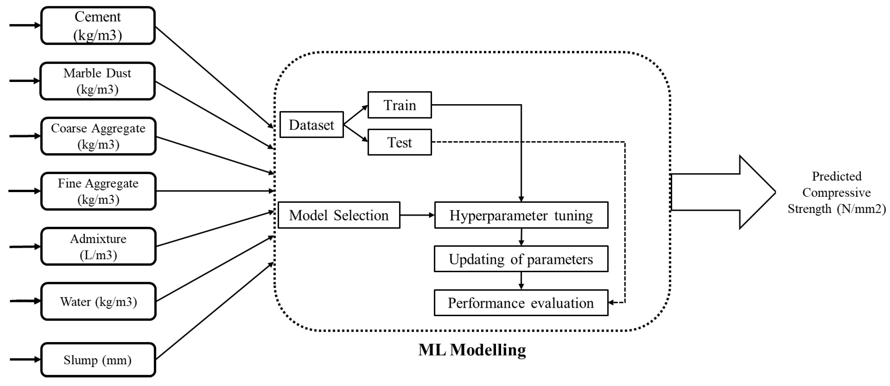
3. Machine Learning Modelling

Different feature compositions contribute to the strength of concrete in different ways. Since the present work aims for estimating the compressive strength of concrete with partial replacement of cement by WMP at various compositions, hence, the problem is treated as that of regression. In the proposed work, we have selected different regression algorithms to analyse the effect of WMP on concrete, viz., Multiple Linear Regression (MLR), K-Nearest Neighbour (KNN), Support Vector Regression (SVR), Decision Tree (DT), Random Forest (RF), Extra Trees (ET) and Gradient Boosting (GB) [22]. For evaluating and comparing efficacy of the applied models, various statistical metrics have been used. These include R${}^2$ Score, MAE, MSE, RMSE, MAPE, MBE which are directly computed using the first and second power of the error in prediction values. The lower value of MAE, MSE, MAPE, MBE and RMSE implies higher accuracy of a regression model. However, a higher value of R square is considered desirable. Another parameter, known as T${}_{stat}$ is also evaluated to analyse the uncertainty level during the prediction.

Considering the total number of samples as N, let y${}_i$ be the original value of ith sample with y${}_i^{{}^{\prime }}$ being its corresponding predicted value. Taking $\overline{y}$ as the average of all the true values, the performance parameters can be calculated as shown in

Table 4. Performance parameters used in the proposed method.

Metric	Formula	Description
R${}^2$	$1-\frac{{\sum }_{i=1}^N{(y_i-y_i^{{}^{\prime }})}^2}{{\sum }_{i=1}^N{(y_i-{\overline{y}}_i)}^2}$	Coefficient of determination: Measure of goodness of the fit
MSE	$\frac{1}{N}{\sum }_{i=1}^N{(y_i-y_i^{{}^{\prime }})}^2$	Mean squared error: Measures closeness of the fitted line to the data points
RMSE	$\sqrt{\frac{1}{N}{\sum }_{i=1}^N{(y_i-y_i^{{}^{\prime }})}^2}$	Root mean squared error: Measures spread of the residuals
MAE	$\frac{1}{N}{\sum }_{i=1}^N\mid y_i-y_i^{{}^{\prime }}\mid$	Mean absolute error: Measures average of absolute differences between true and predicted values
MAPE	$\frac{1}{N}{\sum }_{i=1}^N\mid \frac{y_i-y_i^{{}^{\prime }}}{y_i}\mid$	Mean absolute percentage error: Measures average of absolute percentage differences between true and predicted values
MBE	$\frac{1}{N}{\sum }_{i=1}^N(y_i-y_i^{{}^{\prime }})$	Mean bias error: Measures average of differences between true and predicted values
T${}_{stat}$	$\sqrt{\frac{(N-1)MB{E}^2}{RMS{E}^2-MB{E}^2}}$	t-statistic test: Measures significance of the differences between true and predicted values

. Each modelling technique was performed using in the Python programming language in i5 processor. A generalised process flow for each ML model is shown in Figure 2.

Tuning of hyperparameters for any ML algorithm is considered as a fundamental task for any ML algorithm. Manually estimating the performance of an ML algorithm can be challenging. Additionally, formation of different pairs of hyperparameters is also challenging. Hence, in our work, we have selected a Grid Search Strategy (GSS) so as to automate parameter tuning. GSS accepts manual sets of hyperparameters based on experience to form all exhaustive pairs of different hyperparametes. In order to evaluate performance of one specific pair of hyperparameters, a subset of data, known as validation data, is selected from the training data. Based on the performance on validation data, a set of hyperparameter is selected. GSS is used for all the algorithms mentioned above to generate the best combination of hyperparameters. The following section discusses the applied algorithms for the present work in detail.

3.1. Multiple Linear Regression Model

Multiple Linear Regression MLR model assumes data points, i.e., inputs, to have a liner relationship with the outcome to be estimated. Thus, the model aims to learn a linear dependence of the output variables (compressive strength in our case) on the independent (features) variables, giving the best-fit regression line for the data. Taking into consideration Occam’s razor rule [23], MLR model is applied initially to study the need of exploiting more complex data-driven regression modelling techniques. The output (i.e., concrete strength) is weighted sum of the features used. Weights used in this model are optimized using ordinary least-squares method on the estimated and actual outcomes of training data. This helps in predicting the target values such that the error difference between the predicted and true value is minimum.

3.2. K-Nearest Neighbour

K-nearest neighbour KNN [24] is a non-parametric regression method that is used to approximate the relation between input features and out variable by averaging the observations in the same neighbourhood. It exploits ‘feature similarity’ to predict values of any new data points. In this algorithm, all the training data is stored in memory and similarity between each test instance with the training data is calculated. The most similar K instances are chosen for prediction. The size of the neighbourhood is chosen such that the predicted value is in close proximity to the target value, resulting in minimum errors. In the present work, the KNN regression algorithm takes the number of neighbors (K) and distance metric (d) as its parameters, and considers uniform weights for all the features. In this model, similarity between a test instance with all the training instances is measured using Euclidean distance. The instances with the highest similarity, i.e., minimum distance, are chosen as the K neighbors. The value of K is chosen as 1, 3, 5, 10 and 15% of the total data, thus resulting in K = 8, 22, 36, 72, 108 and 144, respectively.

The model can be very complex for large training data, and may be infeasible to predict when there a large amounts of data.

3.3. Support Vector Regression

Support Vector Regression SVR [25] tries to learn a function that approximates the given input instance to a discrete value output. SVR aims to learn a hyperplane that can distinguish the data points with different outcomes. It is possible that data points may not be separable in lower dimensions. Therefore, a kernel function is used in order to map the data to a higher dimension. Further, there may be multiple hyperplanes that could separate the data points. However, only one particular hyperplane that demonstrate the maximum separation between the outcomes is selected. The separation margin around the hyperplane is termed as boundary. Different parameter in SVR are the type of kernel, regularization parameter (C) and regularization parameter penalty (epsilon) as its parameters. Since the strength of regularization in inversely proportional to C, hence, the value of C has been experimentally chosen to be 10. Further, the regularization parameter penalty helps the optimisation function to obtain optimal solutions by imposing a cost during the training process.

In the present work, L2-loss is used as the type of penalty. Thus, if the error value is less than 0.2 (epsilon), no penalty is associated during regularization. Further, RBF kernel is taken into consideration which assumes non-linearity in separating the training data points.

3.4. Decision Tree

Decision tree DT is a non-linear algorithm, that makes use of tree representation to solve the regression problem. DT employs a “divide and conquer” approach, where a complex task is divided into simpler, regional tasks. A tree is composed of decision nodes (features) and leaves (outcome). Commencing from the root node, each decision node applies a splitting test to the input. Based on the outcome of the test, one of the branches is chosen. The search stops upon reaching a leaf. Each path from the root to a leaf corresponds to a conjunction of different conditions in the decision nodes on the path and such a path can be written as an if–then rule. Thus, a tree can be converted to a rule base of if–then rules that are easy to interpret.

The size of the DT depends on the complexity of the problem underlying the data. Selecting an optimum size of the tree is the major hyper-parameter that can affect the efficiency of the model. Trees with less depth can lead to under-fitting, failing to reach an optimum decision owing to under-training, whereas deeper trees result in models with high complexities.

In the present work, the model considers compressive strength as its leaf node, and the input parameters as its internal nodes. The depth of the tree and splitting criteria are considered as two critical parameters that need to be tuned for best results. In this model, squared error has been selected as the splitting criteria. Tree depths of 1, 2, 3, 4, 5, and 6 have been chosen so as to search for the best parameter.

3.5. Random Forest

Random forest RF is also a non-linear model. As an improvement to the DT algorithm, RF [26] algorithm for regression was introduced, which takes into account the decision of multiple DTs. RF performs bootstrapping to construct multiple subsets of the dataset for each tree. Here, bootstrapping implies sample selection from dataset without replacement. RF is a supervised learning regression algorithm that makes use of ensemble learning by combining predictions from multiple trees so as to make more accurate predictions compared to a single model. Each tree runs individually and in parallel to each other during training time so as to make predictions. The model estimates the compressive strength based on majority voting of multiple trees.

However, similar to DT, optimum choice of tree depths is an important factor for efficient performance. Furthermore, the number of trees in a forest have to be chosen accurately so as to avoid the problem of overfitting.

In the proposed work, 100 trees are considered in the forest. Similar to DT, results for RF model have been studied for tree depths of 1, 2, 3, 4, 5, and 6. This implies that each tree in the forest bears depth.

3.6. Extra Trees

The function of Extra-trees ET regressor [27] is the same as RF, but differs in two ways, viz., selection of the splitting method and bootstrapping. A DT and RF choose the best split whereas ET chooses a random split. Moreover, unlike RF, ET does not perform bootstrapping to construct multiple subsets of the dataset.

3.7. Gradient Boosting

Gradient boosting GB algorithm [28] uses sequence of N number of DTs. A regression model is developed sequentially in order to obtain a strong regression model. First, a DT regression model is trained on using available features and real-valued regression output. Further, the residual to true and estimated real-valued regression output is used for training a new regression model but features remain unchanged. Further, the residual of second model work as the label for the third model. This process is continued until all the trees are trained. During real-time deployment, when a test instance arrives, it is fed to all the trained regression models for estimating the output values. Further multiple outputs are converted to single output values using the parameter `shrinkage’.

4. Experimental Section and Results

The experiments using different ML algorithms were performed and analysed. Results are described in two parts. The first part helps in deciding the regression model that can be used for best prediction of compressive strength of concrete incorporated with WMP. In the latter part, the best chosen regression model is further analysed to study the relevance of each component used in manufacturing of concrete. Further, it would also help in deciding the best proportion of WMP that can replace cement in order to achieve best compressive strength.

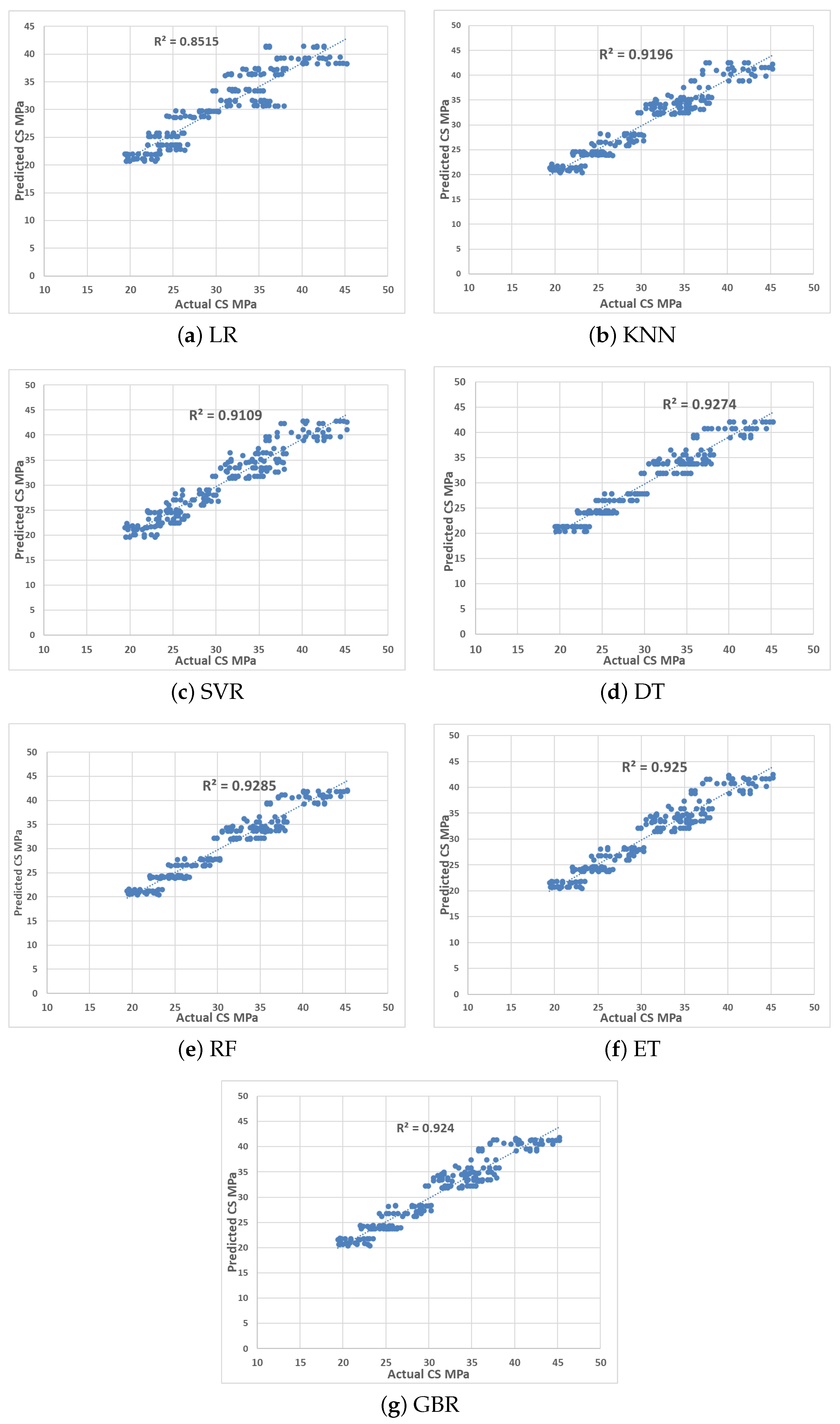
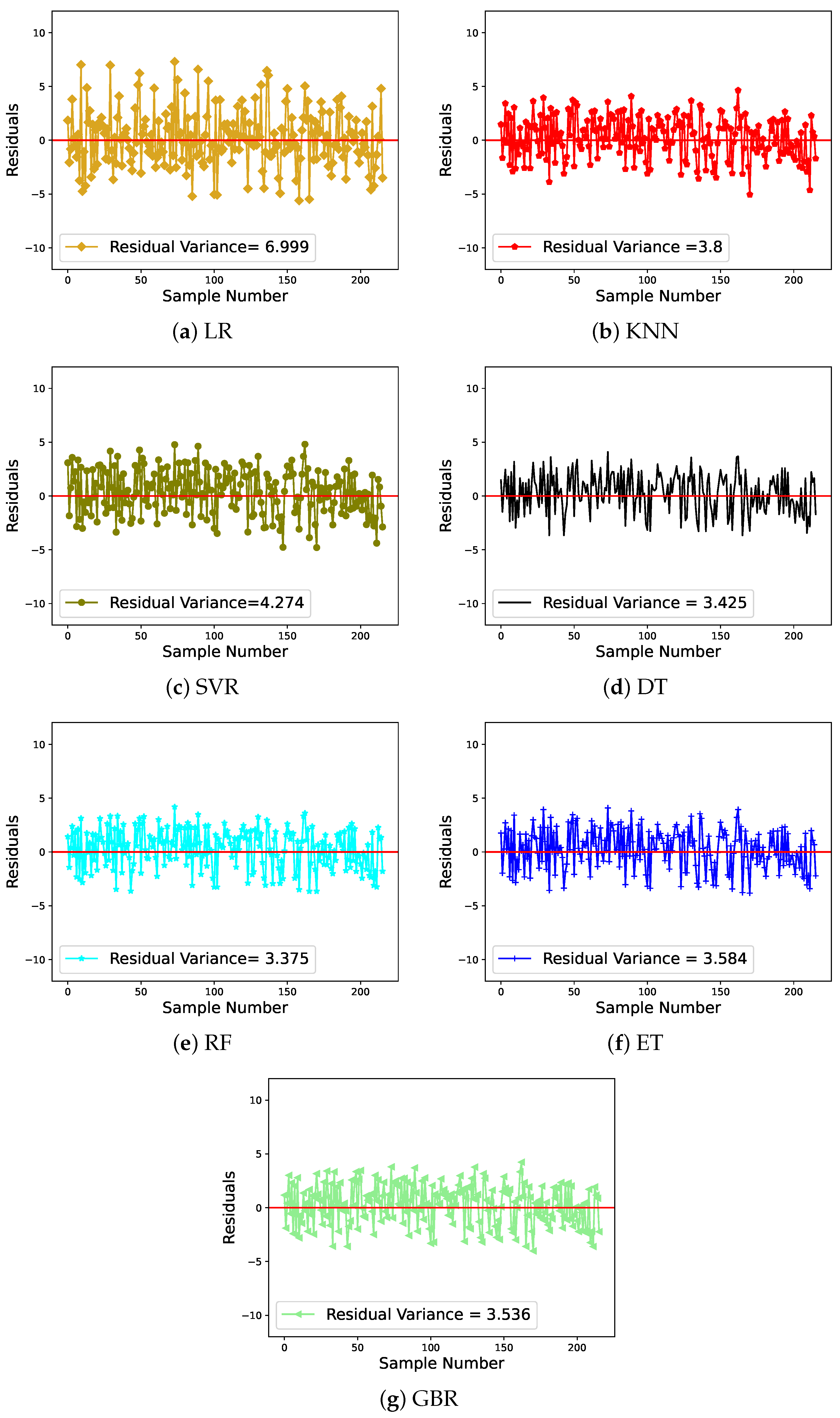
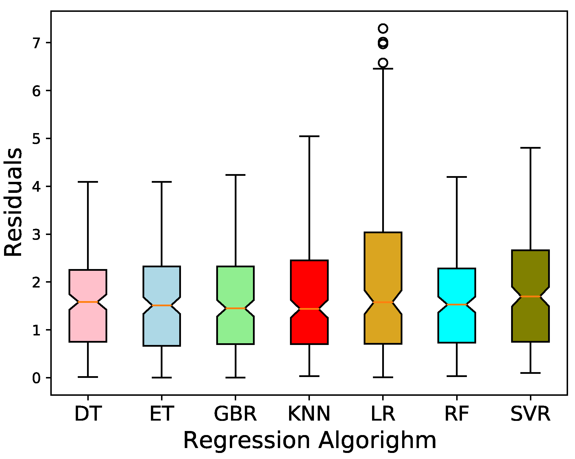
4.1. Results Using Various Regression Models

In order to evaluate the performance of each regression model, the dataset is initially standardized in a manner such that each feature has unit variance zero mean. As described earlier, the data for the current work were collected experimentally by Singh et al. for 12 different sets of design mixes, with each mix considering 5 different marble slurry percentage replacement levels, resulting in 60 variations. A set of 720 data points was generated by casting 12 concrete cubes for each of the 60 variations [21]. From the entire data of 720 samples, 70% is considered for training, while the remaining 30% is used for testing purposes. Further, the experiment on each setup is repeated five times so as to remove any biases from the results and average results have been reported.

Figure 3, Figure 4 and Figure 5 depict the relationships between the true and predicted values for different models. Since a higher R${}^2$ score indicates more perfectly fit data, hence, R${}^2$ values of each regression model have been plotted in the figure. Owing to the lowest R${}^2$ value of 0.852 for the test data, MLR is the least-suited model for predicting compressive strength of cement incorporated with WMP. Furthermore, the model results in maximum fluctuations in prediction (Figure 4), leading to maximum error values as can be seen in Figure 5. Thus, although Occam’s razor rule prioritizes simpler models, in cases where simpler models are unable to perform efficiently, complex ML models prove useful in explaining the variation of dependent variables.

From the figures, it can further be observed that RF algorithm gives the best performance out of all the models with an R${}^2$ value of 0.926. Keeping in mind the increasing complexity of the model with increasing tree depths, a depth of 3 was found to give the best performance. Further, being flexible in nature, it is more convenient for the model to handle larger datasets more efficiently, hence, the method can be efficiently chosen for prediction applications. Moreover, the error graphs (Figure 4 and Figure 5) show that the RF model provides the highest level of accuracy in prediction of compressive strength when compared to the other models. Similarly, for regression analysis using DT model, it was observed that a tree depth of 4 gave the best performance, taking in consideration the saturation in parametric values with increasing tree depths thereafter. For the same, the R${}^2$ value was computed to be 0.924. However, in case of DT, a minute change in data might manifest in the structure of the tree, leading to instability. Moreover, RF algorithm solves the problem of overfitting that might occur in the case of the DT algorithm. Hence, the method is not much preferred to predict compressive strength of concrete from a given set of features.

Although ET and RF algorithms are very similar, the performance of the latter is slightly better than that of the former. Rather, in our case, performance of ET is quite similar to that of DT, with a similar R${}^2$ value of 0.924. However, from Figure 5, it can be seen that predictions vary more from the true compressive strength values in case of ET as compared to RF algorithm. Further, for ET, best results were obtained for a tree depth of 6, which adds to the complexity of the algorithm in comparison to RF and DT, where optimal results were obtained for a tree depth of 3.

While considering GB algorithm, it was observed that the algorithm produces results in performance that is quite similar to ET algorithm with very minute difference of 0.001 in their R${}^2$ values. Although GB is considered as one of the most powerful algorithm for regression applications, the presence of noise in the data makes it difficult for the algorithm to perform well. On the other hand, RF algorithm works efficiently even if data are missing or high noise content is present.

Further, in the case of KNN model, using GSS, the results are best obtained for 1% of neighbours (K), i.e., for K = 8 with R${}^2$ value of 0.919. Since the model finds it difficult to handle noisy data and is sensitive to outliers, thus, with increasing number of neighbours, i.e., with increasing values of K, the error values are also increased. However, being a lazy learner owing to instance-based learning, the model requires all available data in order to make a prediction, thus making it even slower and costly for larger datasets. The results obtained for KNN are comparable to those obtained using SVR algorithm in terms of R${}^2$. It can be observed from Figure 3 that the results for SVR model are better than the MLR model by 6.92%, but underperforms when compared with the rest of the algorithms. Moreover, SVR model requires extensive feature scaling of variables prior to its application, thus making it computationally expensive.

Thus, the results show that the RF model is best suited to predict the compressive strength of concrete, followed by DT models. RF, being a powerful ML algorithm, can result in more accurate predictions when compared to the other algorithms, as can be seen in Figure 4. Furthermore, Figure 5 shows that the RF model gives the least variation in compressive strength values from their true values when compared with other algorithms. Further, it can handle missing data more efficiently and is usually robust to outliers.

Table 5. Performance measures of applied models.

Method	R${}^2$ Score	MAE	MSE	RMSE	MAPE	MBE	t-Stat
MLR	0.852	2.095	7.152	9.455	6.819	0.007	0.191
KNN	0.919	1.655	3.914	9.692	5.427	0.028	0.155
SVR	0.911	1.747	4.380	9.660	5.761	0.048	0.175
DT	0.924	1.632	3.679	9.685	5.370	0.050	0.130
RF	0.926	1.608	3.561	9.679	5.291	0.051	0.126
ET	0.924	1.612	3.668	9.649	5.315	0.017	0.149
GB	0.923	1.621	3.719	9.650	5.333	0.037	0.100

shows different performance measures on the applied models. From the above table, it can be observed that different performance measures consider different ML models as the best performing. The R${}^2$ score, MAE, MSE and MAPE values are the best for RF model. On the other hand, RMSE and MBE values are best shown for MLR, whereas T${}_{stat}$ is best for GB modelling technique. Higher R${}^2$ score for RF indicates that the model best fits the dataset compared to the rest. Further, the model shows least fluctuation in errors, as is indicated by MSE, MAE and MAPE values. This shows that there is minimal variance in residuals for RF model in comparison to the other ML models. Since the RF model is best for the majority of the performance parameters, and the other three parameters, i.e., RMSE, MBE and T${}_{stat}$ do not show any significant best performing model, hence RF was considered for further analysis. Thus, it can be seen that MLR is the least preferred model for regression since all the performance measures except RMSE and MBE are least preferred, thus leading to the need of more complex models for prediction. Furthermore, with exponentially increasing data in the current scenario, the applicability of MLR becomes minimal. Further, RF model gives the best estimation of compressive strength of concrete with partial replacement of cement by WMP. The overall performance of RF is higher when compared to the rest of the models. Other methods, compared to the rest of the methods, such as DT and ET can be considered as the next choice, but only in cases where data complexity is low.

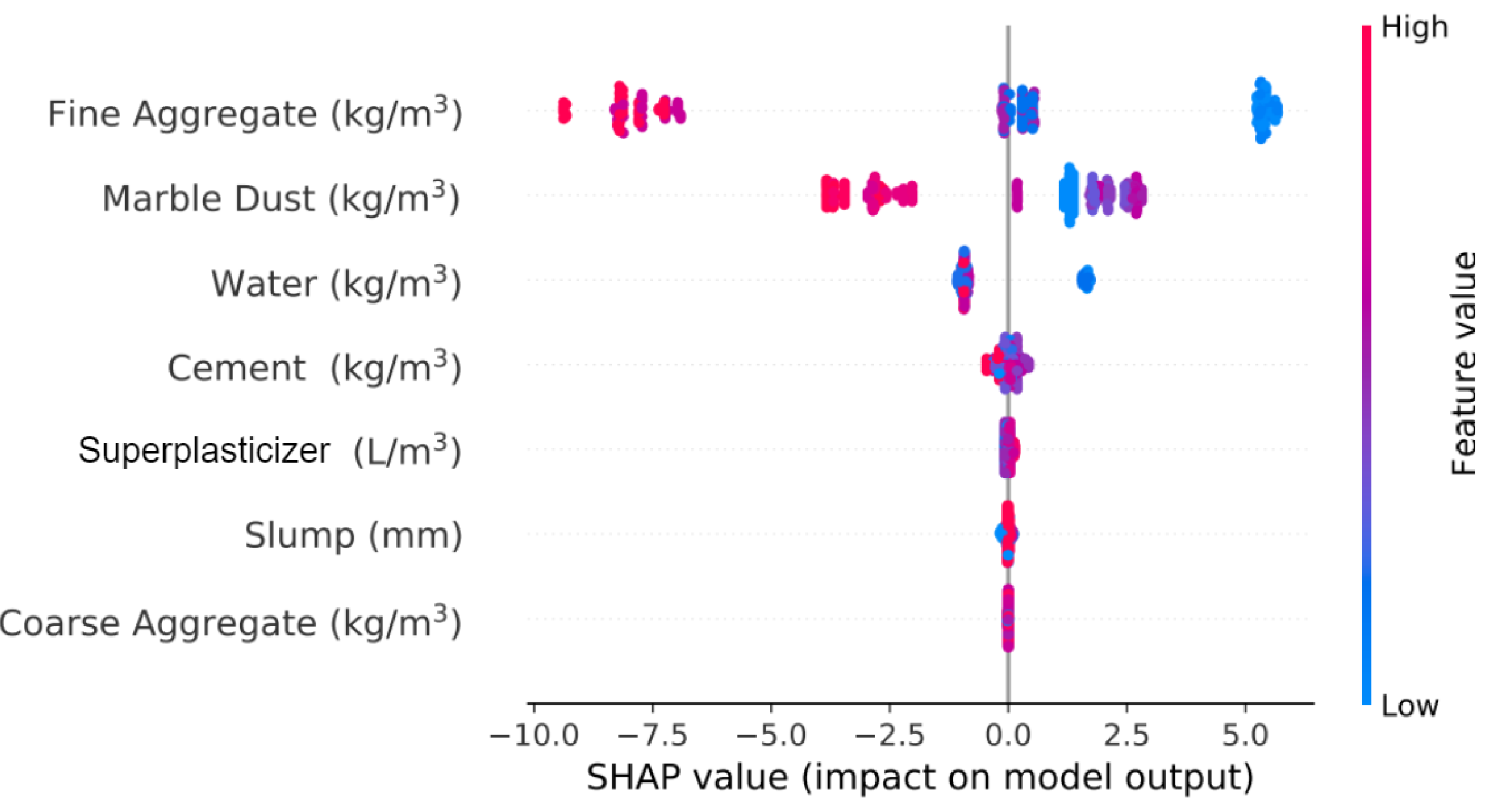
4.2. Analysis of the Best Model

Each independent variable has its own contribution in deciding its effect on the compressive strength of concrete. Since RF regression technique exhibited best performance among all the models tested, the importance of features was analysed using the same. Average results are shown in the form of Variance Inflation Factor (VIF) in Figure 6. A VIF of 1 indicates that the corresponding feature has no correlation with any of the other features. Typically, a VIF value exceeding 5 or 10 is deemed too high. Any feature with such high VIF value is likely to be contributing to multicollinearity. As has been discussed in the literature and also shown by Singh et al. [21], marble dust does not explicitly affect the hydration process. Rather, it mainly works as a filler by also providing nucleation sites for enhanced hydration products. Accordingly, the contribution of marble dust on compressive strength has been found lesser as compared to the other input variables, although not entirely negligible (8%).

SHapley Additive exPlanations (SHAP) is used further for explaining the compound learned decision functions used by RF Technique as shown in Figure 7, where y-axis shows features used for the model, while the x-axis shows the impact of the corresponding feature on the model output. The position of feature between the peak and lowest values is indicated by the colour. Overlapping points show the density of Shapley values per feature. According to the figure, the RF technique is highly sensitive to WMP and fine aggregate content. Overall, mainly water, marble dust and fine aggregate contents are being used for prediction, followed by cement, superplasticizer admixture and Slump content.

Thus, from the overall analysis, it can be said that marble-slurry-incorporated concrete results in an improvement in mechanical properties at 15% replacement by weight of cement as compared to control mix for lower water–binder ratio of 0.35 and 0.40. For the water–binder ratio of 0.45, compressive strength is improved only up to a maximum replacement of 10%. Further, with the simultaneous increment in the dosage ofsuperplasticizer and marble slurry, higher strength magnitude is observed as compared to constant dosage, owing to compactive power of superplasticizer admixture. This improvement is observed from the acceleration effect of WMP on the hydration process, which is further related to the formation of calcium carboaluminate hydrates. Furthermore, the improvement in binding capacity of carboaluminate is likely due to its compact structure as described by Bonavetti et al. [29]. Singh et al. [21] demonstrated the compaction and decreased porosity of concrete on use of marble powder using Scanning Electron Microscopy (SEM) images. Further, SHAP dependency plots help to obtain a deeper insight into the spread and variation of the predicted CS values with respect to the content of WMP as well as fine aggregate and water content being the main ingredients.

5. Conclusions

On replacing cement with marble dust, there may be a dilution effect causing a reduction in the strength of concrete for varying water–binder ratios [21]. Thus, optimizing the content of marble dust is key. In this study, the compressive strength of concrete incorporated with WMP has been predicted using different ML algorithms. The estimation of compressive strength for different compositions of concrete is considered to be a regression problem. Data were collected from experimental trials using Ordinary Portland cement (OPC 43) replaced with WMP in different proportions. Performances using different regression models, viz., KNN, SVR, DT, RF, ET, GB and MLR, have been analysed and reported. Results show that the RF model is best suited to predict the compressive strength of concrete, followed by ET and DT models. Thus, RF can help in efficiently calculating the amount of WMP that can replace cement without affecting the compressive strength of concrete for practical applications. Further, on analysing the best obtained model, it can be concluded that WMP contributes approximately 8% to the total compressive strength of concrete. The data-driven models may help in predicting the strength based on input and output variables and also apply them to a large-scale dataset. However, there is no guarantee that they will explain the causality of the relationships accurately in prediction. The error may be significantly lower; however, the chemical reactions and changes taking place may not be completely predictable. These models may be used to understand the complex behaviour of marble dust which in turn would help to maximize its benefits in the construction industry. Notwithstanding, model robustness when faced with entirely new samples should be taken into consideration in this type of analysis as a calibrated model on a data point with a different structure.

References

1. Kore, S.D.; Vyas, A. Impact of marble waste as coarse aggregate on properties of lean cement concrete. Case Stud. Constr. Mater. 2016, 4, 85–92. [Google Scholar] [CrossRef] [Green Version]
2. Pappu, A.; Thakur, V.K.; Patidar, R.; Asolekar, S.R.; Saxena, M. Recycling marble wastes and Jarosite wastes into sustainable hybrid composite materials and validation through Response Surface Methodology. J. Clean. Prod. 2019, 240, 118249. [Google Scholar] [CrossRef]
3. Rana, A.; Kalla, P.; Csetenyi, L.J. Sustainable use of marble slurry in concrete. J. Clean. Prod. 2015, 94, 304–311. [Google Scholar] [CrossRef]
4. Shamsabadi, E.A.; Roshan, N.; Hadigheh, S.A.; Nehdi, M.L.; Khodabakhshian, A.; Ghalehnovi, M. Machine learning-based compressive strength modelling of concrete incorporating waste marble powder. Constr. Build. Mater. 2022, 324, 126592. [Google Scholar] [CrossRef]
5. Karimipour, A.; Jahangir, H.; Eidgahee, D.R. A thorough study on the effect of red mud, granite, limestone and marble slurry powder on the strengths of steel fibres-reinforced self-consolidation concrete: Experimental and numerical prediction. J. Build. Eng. 2021, 44, 103398. [Google Scholar] [CrossRef]
6. Chu, H.H.; Khan, M.A.; Javed, M.; Zafar, A.; Khan, M.I.; Alabduljabbar, H.; Qayyum, S. Sustainable use of fly-ash: Use of gene-expression programming (GEP) and multi-expression programming (MEP) for forecasting the compressive strength geopolymer concrete. Ain Shams Eng. J. 2021, 12, 3603–3617. [Google Scholar] [CrossRef]
7. al Swaidani, A.M.; Khwies, W.T. Applicability of artificial neural networks to predict mechanical and permeability properties of volcanic scoria-based concrete. Adv. Civ. Eng. 2018, 2018, 1–16. [Google Scholar] [CrossRef]
8. Chithra, S.; Kumar, S.S.; Chinnaraju, K.; Ashmita, F.A. A comparative study on the compressive strength prediction models for High Performance Concrete containing nano silica and copper slag using regression analysis and Artificial Neural Networks. Constr. Build. Mater. 2016, 114, 528–535. [Google Scholar] [CrossRef]
9. Eskandari-Naddaf, H.; Kazemi, R. ANN prediction of cement mortar compressive strength, influence of cement strength class. Constr. Build. Mater. 2017, 138, 1–11. [Google Scholar] [CrossRef]
10. Naderpour, H.; Rafiean, A.H.; Fakharian, P. Compressive strength prediction of environmentally friendly concrete using artificial neural networks. J. Build. Eng. 2018, 16, 213–219. [Google Scholar] [CrossRef]
11. Vakhshouri, B.; Nejadi, S. Prediction of compressive strength of self-compacting concrete by ANFIS models. Neurocomputing 2018, 280, 13–22. [Google Scholar] [CrossRef]
12. Duan, Z.H.; Kou, S.C.; Poon, C.S. Using artificial neural networks for predicting the elastic modulus of recycled aggregate concrete. Constr. Build. Mater. 2013, 44, 524–532. [Google Scholar] [CrossRef]
13. Deng, F.; He, Y.; Zhou, S.; Yu, Y.; Cheng, H.; Wu, X. Compressive strength prediction of recycled concrete based on deep learning. Constr. Build. Mater. 2018, 175, 562–569. [Google Scholar] [CrossRef]
14. Ly, H.B.; Nguyen, T.A.; Tran, V.Q. Development of deep neural network model to predict the compressive strength of rubber concrete. Constr. Build. Mater. 2021, 301, 124081. [Google Scholar] [CrossRef]
15. Nunez, I.; Marani, A.; Flah, M.; Nehdi, M.L. Estimating compressive strength of modern concrete mixtures using computational intelligence: A systematic review. Constr. Build. Mater. 2021, 310, 125279. [Google Scholar] [CrossRef]
16. Mansouri, I.; Ozbakkaloglu, T.; Kisi, O.; Xie, T. Predicting behavior of FRP-confined concrete using neuro fuzzy, neural network, multivariate adaptive regression splines and M5 model tree techniques. Mater. Struct. 2016, 49, 4319–4334. [Google Scholar] [CrossRef]
17. Sahoo, S.; Mahapatra, T.R. ANN Modeling to study strength loss of Fly Ash Concrete against Long term Sulphate Attack. Mater. Today: Proc. 2018, 5, 24595–24604. [Google Scholar] [CrossRef]
18. Khan, M.A.; Zafar, A.; Farooq, F.; Javed, M.F.; Alyousef, R.; Alabduljabbar, H.; Khan, M.I. Geopolymer concrete compressive strength via artificial neural network, adaptive neuro fuzzy interface system, and gene expression programming with K-fold cross validation. Front. Mater. 2021, 8, 621163. [Google Scholar] [CrossRef]
19. Aliabdo, A.A.; Abd Elmoaty, M.; Auda, E.M. Re-use of waste marble dust in the production of cement and concrete. Constr. Build. Mater. 2014, 50, 28–41. [Google Scholar] [CrossRef]
20. Santos, T.; Gonçalves, J.P.; Andrade, H. Partial replacement of cement with granular marble residue: Effects on the properties of cement pastes and reduction of CO2 emission. SN Appl. Sci. 2020, 2, 1–12. [Google Scholar] [CrossRef]
21. Singh, M.; Srivastava, A.; Bhunia, D. An investigation on effect of partial replacement of cement by waste marble slurry. Constr. Build. Mater. 2017, 134, 471–488. [Google Scholar] [CrossRef]
22. Alpaydin, E. Introduction to Machine Learning; MIT Press: Cambridge, MA, United States, 2020. [Google Scholar]
23. Witten, I.H.; Frank, E.; Hall, M.A.; Pal, C.J.; DATA, M. Practical machine learning tools and techniques. In Proceedings of the Data Mining; Elsevier International Publishing: Amsterdam, The Netherlands, 2005; Volume 2. [Google Scholar]
24. Altman, N.S. An introduction to kernel and nearest-neighbor nonparametric regression. Am. Stat. 1992, 46, 175–185. [Google Scholar]
25. Cortes, C.; Vapnik, V. Support-vector networks. Mach. Learn. 1995, 20, 273–297. [Google Scholar] [CrossRef]
26. Breiman, L. Random forests. Mach. Learn. 2001, 45, 5–32. [Google Scholar] [CrossRef] [Green Version]
27. Basu, V. Prediction of Stellar Age with the Help of Extra-Trees Regressor in Machine Learning. In Proceedings of the International Conference on Innovative Computing & Communications (ICICC), West Bengal, India, 29 March 2020. [Google Scholar]
28. Zhang, Y.; Haghani, A. A gradient boosting method to improve travel time prediction. Transp. Res. Part Emerg. Technol. 2015, 58, 308–324. [Google Scholar] [CrossRef]
29. Bonavetti, V.; Rahhal, V.; Irassar, E. Studies on the carboaluminate formation in limestone filler-blended cements. Cem. Concr. Res. 2001, 31, 853–859. [Google Scholar] [CrossRef]
Figure 1. (ag) Correlation between input variables and compressive strength; (h) Correlation between various input variables.
Coatings 13 00066 g001aCoatings 13 00066 g001b
Figure 2. Process flow for various ML algorithms.
Coatings 13 00066 g002
Figure 3. Performance of various ML models in CS prediction.
Coatings 13 00066 g003
Figure 4. Fluctuations in errors, the model showing the least fluctuations represents the desirable outcome.
Coatings 13 00066 g004
Figure 5. Error bound analysis, where the residuals are computed by taking absolute difference of true and estimated values.
Coatings 13 00066 g005
Figure 6. VIF analysis for RF.
Coatings 13 00066 g006
Figure 7. SHAP analysis.
Coatings 13 00066 g007