Machining of Carbon Steel under Aqueous Environment: Investigations into Some Performance Measures

Abstract

In this study, a new machining approach (aqueous machining) is applied for mill machining and its performance is compared with traditional wet machining. AISI 1020 steel is employed as the test material and Taguchi statistical methodology is implemented to analyze and compare the performance of the two machining approaches. The cutting speed, feed rate, and depth of cut were the machining parameters used for both types of machining, while the selected response variables were surface roughness and hardness. Temperature variations were also recorded in aqueous machining. Compared with wet machining, aqueous machining resulted in lower surface roughness (up to 13%) for the same operating conditions and about 14% to 16% enhancement in hardness due to the formation of finer pearlite, as revealed by the microstructure analysis. Compared to the parent unmachined surface, the hardness of machined surfaces was 24% to 31% higher in wet machining and 44% to 51% higher in aqueous machining. Another benefit of aqueous machining was the energy gain, which ranged from 718 to 8615.96 J. This amount of heat energy can be used as waste heat for preheating domestic hot water, running the organic Rankine cycle with waste heat and preheating the inlet saline water for desalination, vacuum desalination, etc. If successfully implemented in the future, this idea will provide a step towards achieving sustainable machining by saving lubricants and toxic wastes in addition to saving energy for secondary applications.

1. Introduction

The machining process has been an essential part of the industry since the industrial revolution [1,2]. Milling is a broadly used machining process in various manufacturing industries [3]. It is famous for its flexibility and capacity to accomplish exact output compared to other processes. It produces a machined surface by removing a pre-defined amount of thickness of material from the workpiece [4]. End milling is extensively employed in manufacturing, particularly in the automotive sector. In the end milling process, due to the friction of the workpiece and tool, a considerable quantity of heat is produced, which results in a change in the properties of the material. Hence, the intense tool-to-workpiece contact may create significant temperatures in the process zone in milling processes [5]. Therefore, researchers have employed new coolant and machining strategies to remove the amount of heat from the process zone generated in machining processes [6,7,8,9]. Similarly, various cutting fluids have been proposed to remove friction, which is directly applied at the interface of the workpiece and tool during the machining process [10]. Therefore, problems such as dimensional variance, surface roughness, poor finishing, temperature, etc., need further investigation [11].

For instance, Al Hazza et al. [12] established multiple regression prediction models to foresee surface quality in end milling. The factors selected for the study are depth of cut, feed rate, and spindle speed. When this model was applied, the result was impressive and predicted surface roughness with 90% accuracy. Out of the remaining input parameters, the feed rate was the most important factor noticed in this model. Cutting speed, feed rate, and a milling depth of cut were tested experimentally to compare conventional and ultrasonic vibration-assisted milling, to evaluate the efficacy in raising the value of machined surface roughness for hardened AISI H11 tool steel by Mejbel et al. [13]. Up to 89% lower roughness was achieved using axial ultrasonic-assisted vibration in milling compared to the traditional milling method with the same cutting conditions, resulting in better surface finish and quality. Raju and Gedela [14] examined three basic parameters, feed rate, spindle speed, and depth of cut, as input factors and surface roughness and material removal rate (MRR) as output parameters. It was observed that for Aluminum 6063, the most effective parameter on surface roughness was spindle speed, with 31% contribution, and that of material removal rate was feed rate, with 35.99% contribution. Similarly, for Aluminum A380, the feed rate with a 34.78% contribution was the most effective parameter on surface roughness. Additionally, the feed rate was the most effective parameter (34.30%) in the material removal rate. Philip et al. [15] employed the response surface methodology (RSM) to study the effects of the spindle speed, axial depth of cut, and feed rate of duplex stainless steel. After applying the response surface methodology, it was concluded that the feed rate was the most prominent factor affecting the output. The axial depth of cut was the second most effective parameter and spindle speed was the last parameter that affected the output parameters. Rawangwong et al. [16] used semi-solid AA7075 for experimentation with a carbide tool on CNC milling vertical machine. A factorial design was employed in this research. The outcomes of the runs showed that feed rate and speed were the factors that affect the output parameters, whereas the effects of the depth of cut remain negligible. Similarly, Tian et al. [17] used a carbide cutting tool for milling Titanium alloy TC-17. The purpose of this was to see the behavior of milling parameters on surface hardness.

The process by which coolant is provided by an external source such as pumps and motors is called wet machining. Another new type of machining proposed in this study is aqueous machining, in which the workpiece is completely dipped into coolant and machining takes place in an aqueous environment, providing an opportunity to reduce friction and heat generation directly. The present study focuses on the comparative analysis of aqueous machining vs. wet machining for surface quality and hardness of the machined components. Additionally, optimization of parameters for reduced surface roughness and desirable hardness values were carried out using mean effect plots employing the Taguchi approach. After wet and aqueous machining, the hardness of the finished part has been compared to check essential alterations in its properties. The effect of the cooling environment on the microstructure of AISI 1020 steel is also examined using an optical microscope. The study also focuses on the recovery of waste heat generated during the aqueous machining by workpiece and chip production. More specifically, the amount of energy recovered during this machining process puts stress on the sustainability of the machining process.

2. Materials and Methods

2.1. Material and Machine

AISI 1020 steel was chosen for this study due to its low cost, availability, and wide industrial applications. The chemical composition of AISI 1020 steel, as provided by the supplier, is shown in

Table 1. Chemical composition of AISI 1020 steel.

Chemical Composition wt.%
C	Si	Mn	S	P	Mo
0.17	0.12	0.48	0.031	0.014	0.018

. The mechanical and physical properties of the tested workpiece are given in

Table 2. Mechanical and physical properties of AISI 1020 steel.

Properties of AISI 1020 Steel
Young’s modulus (GPa)	186
Density (kg/m3)	7.87
Modulus of rigidity (GPa)	72
Yield strength (N/mm2)	384
Poisson’s ratio	0.29
Thermal conductivity (W/km)	51.9
Coefficient of thermal expansion (µm/m-°C)	11.7
Specific heat capacity (J/g-°C)	0.486

. The dimensions of the sample prepared were 15 mm × 90 mm × 50 mm. The Bridgeport Series 1 CNC milling was employed for conducting the tests.

2.2. Tool and Coolants

For cutting the material, a 4-flute flat-end HSS (High-Speed Steel) mill cutter coated with TiAIN (diameter 8 mm) was utilized for both types of machining. The coolants in machining were mainly aimed at cooling and/or lubricating the area of interaction of the tool and the material being machined. Soluble oils need to be mixed with water to effectively provide lubrication and heat removal purpose. Cutting fluids are generally the mixture of water and oil in a predefined ratio ranging from 10:1 to 50:1. In this research, vegetable-based cutting fluid (VBCF) was mixed with water at a ratio of 15:1 and was used in experiments. In the case of wet machining, flood cooling with a flow rate of 0.48 mL/min was exercised. However, in the case of submerged machining, a tank made up of acrylic sheets (280 mm × 170 mm × 150 mm) was prepared and utilized, as shown in Figure 1. Moreover, to fasten the tank firmly onto the bed of the CNC mill, two holes were created at the bottom and were sealed using an industrial-grade sealant. The volume of the coolant was 280 mm × 30 mm × 170 mm = 1,428,000 mm³.

2.3. Surface Roughness Measurement

The surface roughness was measured across the tool travel direction, as it is believed to be larger in this direction. For this purpose, Surftest SJ-201 (Mitutoyo, USA) portable surface roughness tester was used, and its stylus was made to travel over the machined surface by 5 mm. This is because the mean roughness is assumed to be a good indicator of surface finish in machining. The surface roughness (Ra) tests were repeated at eight different locations on the surface to obtain precise results, and the average (R_a) was analyzed.

2.4. Hardness Measurement

The microhardness of the machined and unmachined surfaces was measured using the Vickers Hardness (HV) Tester, Tukon 300. The indentations were performed by applying the pressure of 1 kg. Before performing hardness tests, the surfaces were gently cleaned with fine abrasive sandpaper to remove the machining asperities. Then, hardness was measured at five different points of the machined area and an average of all the measured values to obtain a more accurate result.

2.5. Temperature Measurement

In the present study, temperature measurements were restricted to the coolant in the tank in aqueous machining. The purpose was to find the energy gain that one can realize due to machining for onward use in any secondary processing (say water heating etc.). For this purpose, DS18B20 Waterproof Temperature Sensor and Arduino Mega 2560 were used to record the temperature variation(s). The accuracy of the DS18B20 is ±0.5 °C in the temperature range of −10 °C to +85 °C.

2.6. Design of Experimental Plan

The two machining processes, i.e., aqueous machining and wet machining, were conducted with varying parameters. The Design of Experiments (DoE) approach with Taguchi design was employed. Taguchi’s approach requires less tests than the conventional full factorial design. This method has been functional in the production industries to identify the effect of the machining parameters on performance. The selection of input parameters and the number of levels is the most important stage in Taguchi’s approach, based on which an orthogonal array is selected to conduct experimental runs [18]. For the milling process, the main variables are the depth of cut, feed rate, and spindle speed, as shown in

Table 3. Selection of levels.

Parameters	Level 1	Level 2	Level 3
Depth of cut (mm): A	0.2	0.3	0.4
Feed rate (mm/min): B	300	500	800
Spindle speed (rpm): C	1200	1500	1800

.

The first step of Taguchi’s design was done by selecting the orthogonal array (L₉) that includes nine experimental runs to examine the effect of three input parameters on the output variables. The orthogonal array of nine experimental runs was generated Using Minitab software. Based on the Taguchi design, the complete test plan is presented in

Table 4. Taguchi orthogonal array.

Run	Depth of Cut: A	Feed Rate: B	Spindle Speed: C
1	1	1	1
2	1	2	2
3	1	3	3
4	2	1	2
5	2	2	3
6	2	3	1
7	3	1	3
8	3	2	1
9	3	3	2

.

3. Results

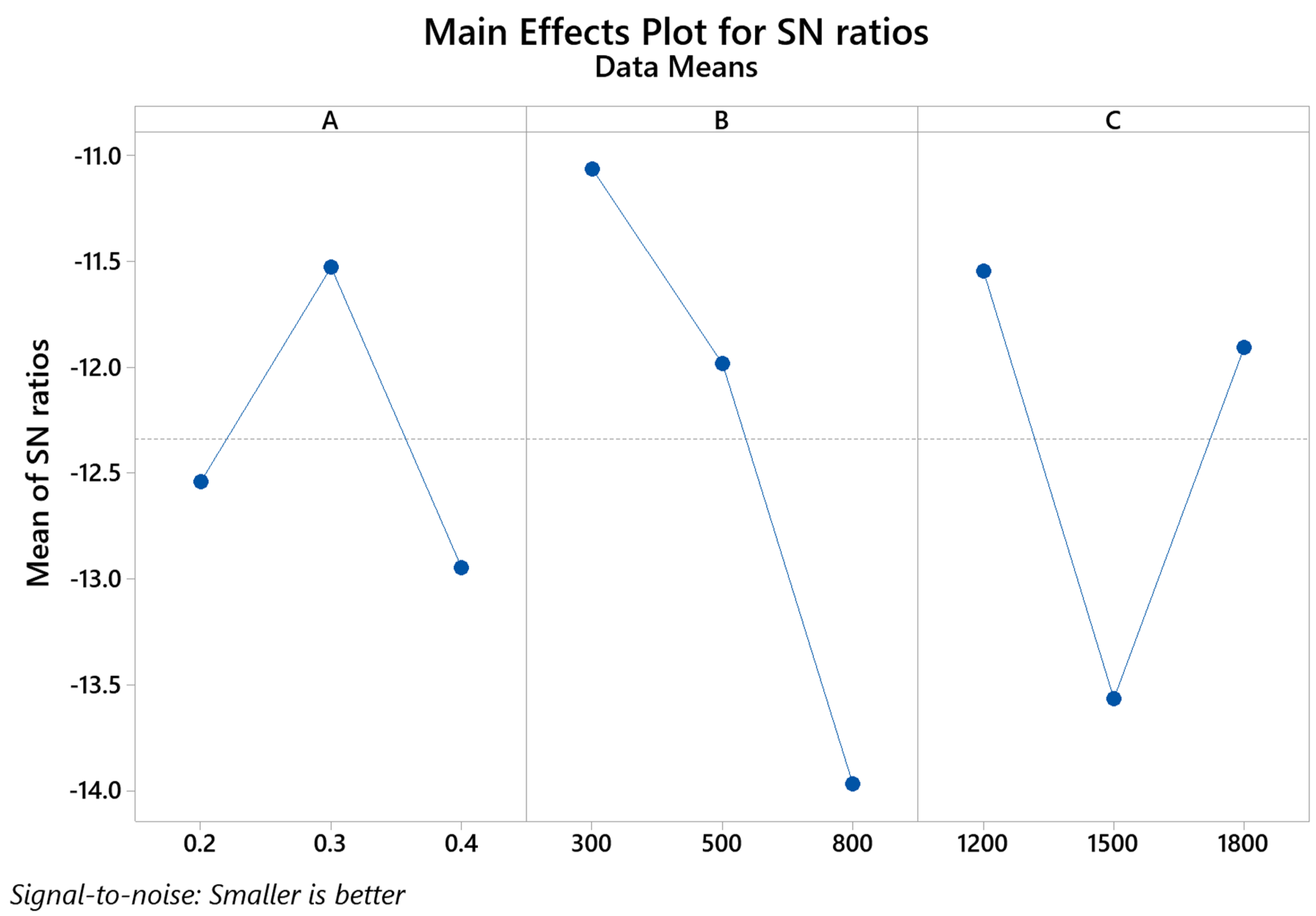
3.1. Analysis of Surface Roughness in Aqueous and Wet Machining

In this study, statistical analysis using Minitab software was performed to identify the effect of parameters on roughness in each machining method, and the Signal/Noise (S/N) ratios were estimated. As lower values of surface roughness are required, the “smaller the better” was employed as a criterion in this case, as given in Equation (1):

$$\mathsf{\eta }=-10\times \log \left[\frac{1}{n}\left({\displaystyle \sum }{Y}^2\right)\right]$$

(1)

where Y is the result for factor-level assigned for runs and n is the number of results for factor-level assigned for runs [19].

Table 5. Experimental mean and S/N values of surface roughness.

Roughness Values (µm)
Parameters				Wet Machining		Aqueous Machining
Run	A	B	C	Mean Values	S/N Values	Mean Values	S/N Values
1	0.2	300	1200	3.402	−10.63	3.328	−10.44
2	0.2	500	1500	4.887	−13.78	5.371	−14.6
3	0.2	800	1800	4.575	−13.21	4.305	−12.68
4	0.3	300	1500	3.527	−10.95	3.469	−10.8
5	0.3	500	1800	3.508	−10.9	3.445	−10.74
6	0.3	800	1200	4.332	−12.73	3.356	−10.52
7	0.4	300	1800	3.804	−11.61	3.682	−11.32
8	0.4	500	1200	3.659	−11.27	3.556	−11.02
9	0.4	800	1500	6.285	−15.97	5.272	−14.44

A—Depth of cut (mm), B—Feed rate (mm/min), C—Spindle speed (rpm).

shows the experimental mean values and the S/N values for surface roughness during wet and aqueous machining.

Figure 2 shows the main effects plots for surface roughness of wet machined surfaces. The plot shows that the feed rate is one of the most important parameters affecting the roughness because it largely deviates from the mean compared to other parameters. The second and third essential parameters include spindle speed and depth of cut, respectively. The main effect plots for the surface roughness of the aqueous machined surfaces are given in Figure 3. The spindle speed was one of the most important parameters affecting roughness in aqueous machining, contrary to the feed rate in wet machining. At the same time, the depth of cut was found to be the second influential parameter, followed by feed rate.

Table 6. Optimal parameters for surface roughness.

Surface Roughness: Wet Machining
	Depth of cut: A	Feed rate: B	Spindle speed: C
Level	2	1	1
Values	0.30 (mm)	300 (mm/min)	1200 (rpm)
Surface Roughness: Aqueous Machining
	Depth of cut: A	Feed rate: B	Spindle speed: C
Level	2	1	1
Values	0.30 (mm)	300 (mm/min)	1200 (rpm)

shows the optimized parameters for the surface roughness in the wet and aqueous machining processes. Hence, the optimum condition minimizing the roughness is the same in both methods. However, the order of significance of parameters affecting the surface roughness was slightly different.

As the parameters selected for experiments in wet machining and aqueous machining were the same, a comparative analysis can therefore be carried out, as given in Figure 4. The mean roughness in wet machining ranges from 3.4 μm to 6.29 μm, and that in aqueous machining ranges from 3.33 μm to 5.27 μm. The results show that aqueous machining offers improved surface quality as the mean roughness of the related machined surfaces is generally lower. As estimated from the shown data, the former method can reduce the roughness by up to 13%. Hence, aqueous machining offers better surface quality than the conventional wet machining method.

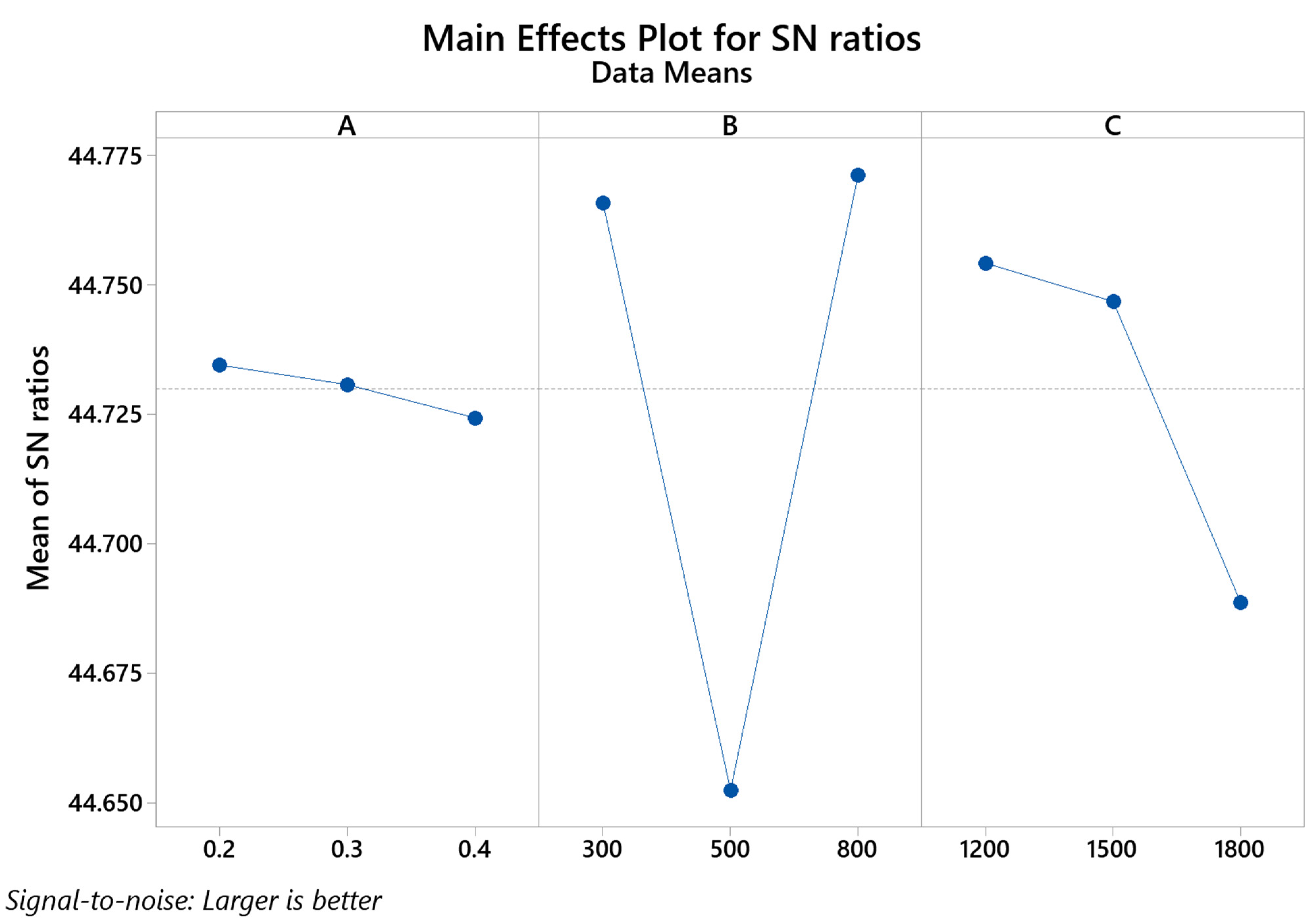
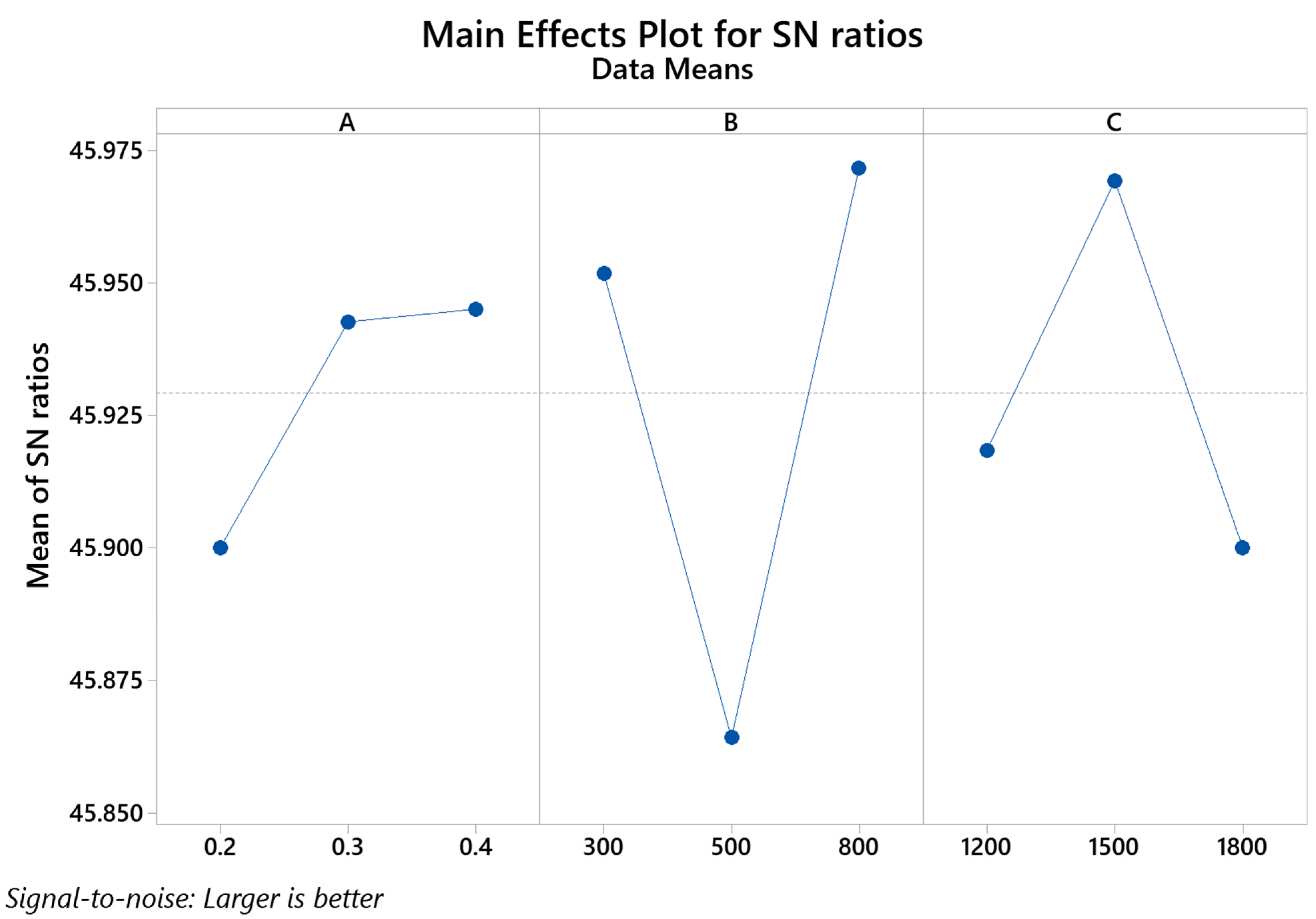
3.2. Analysis of Hardness in Aqueous and Wet Machining

The experimental mean values for hardness values during the wet and aqueous machining are given in

Table 7. Experimental mean and S/N values of hardness.

Hardness Values (HV)
Parameters				Wet Machining		Aqueous Machining
Run	A	B	C	Mean Values	S/N Values	Mean Values	S/N Values
1	0.2	300	1200	170.96	44.6579	201.26	46.0751
2	0.2	500	1500	173.30	44.7760	196.86	45.8831
3	0.2	800	1800	173.18	44.7700	193.68	45.7417
4	0.3	300	1500	174.16	44.8190	195.74	45.8336
5	0.3	500	1800	167.40	44.4751	199.80	46.0119
6	0.3	800	1200	175.76	44.8984	199.12	45.9823
7	0.4	300	1800	174.20	44.8210	198.30	45.9465
8	0.4	500	1200	171.92	44.7065	192.70	45.6976
9	0.4	800	1500	170.72	44.6457	203.96	46.1909

A—Depth of cut (mm), B—Feed rate (mm/min), C—Spindle speed (rpm).

. For the hardness analysis, the “larger-the-better” criterion for hardness was used and the S/N ratio was estimated using Equation (2) [19]:

$$\mathsf{\eta }=-10\times \log {\displaystyle \sum }\left[\frac{1/Y^2}{n}\right]$$

(2)

where Y is the result for factor-level assigned for runs and n is the number of results for factor-level assigned for runs. Table 7 also shows the S/N values of the hardness in wet and aqueous machining surfaces.

Figure 5 shows the main effect plot for the hardness of the wet machined surfaces, whereas the main effect plot for hardness of the aqueous machine surface is shown in Figure 6. It is evident from the plots that feed rate was the most prominent factor on the hardness, followed by spindle speed and depth of cut in both machining processes. It is worth pointing out that the two machining methods follow the same order of significance of parameters. The optimized parameters giving the highest hardness for the wet machining are somehow different from the aqueous machining, as shown in

Table 8. Optimal parameters for hardness.

Hardness: Wet Machining
	Depth of cut: A	Feed rate: B	Spindle speed: C
Level	1	3	1
Values	0.20 mm	800 mm/min	1200 rpm
Hardness: Aqueous Machining
	Depth of cut: A	Feed rate: B	Spindle speed: C
Level	3	3	2
Values	0.40 mm	800 mm/min	1500 rpm

.

Hardness is an essential property of steel. As the workpieces were machined under the cooling environment, the hardness of the machined surfaces is likely to change with respect to the parent metal. The hardness of the parent unmachined metal was recorded to be 134.6 HV. After machining, the hardness of wet machined surfaces varies from 167.4 HV to 175.8 HV and the hardness of aqueous machined surfaces varies from 194 HV to 204 HV. This represents the fact that hardness increased by 24% to 31% in wet machining and 44% to 51% in aqueous machining. Figure 7 compares the hardness of the two machining methods. As estimated, the hardness of aqueous machined surfaces is greater (l4% to 16%) than that of the wet machined surfaces throughout the range of investigation. Therefore, the aqueous machining method offers better hardness than the conventional wet machining method.

3.3. Microstructure Analysis

To study the effect of the cooling environment on the microstructure of steel, samples were cut section-wise and grounded using abrasive water paper up to 2400 grit, followed by mechanical polishing using 1-micron diamond suspension paste. The samples were then etched for a few seconds using a solution composed of 2 mL nitric acid in 98 mL ethanol. Finally, the samples were studied under Olympus BH2-UMA optical microscope. In addition, the metallographic examination has been carried out for two samples showing maximum hardness results after both types of machining.

Figure 8a–d shows the optical micrographs of thickness sections of S9 (Aqueous machining experiment no. 09) and W6 (Wet machining experiment no. 06) samples, respectively. The dark areas represent the pearlite matrix, while the bright areas signify the ferrite (indicated with arrows). The examination of these micrographs reveals that the pearlite phase is denser at the machined edge in comparison to the core of the material, thereby revealing that the surface layers of the material underwent phase transformation during machining. Further, the pearlite and ferrite on edge are relatively finer due to the rapid cooling of ferrite (pre-eutectoid) and austenite (γ). This explains why the hardness of the machined surfaces, as found earlier, is greater than the unmachined surface. It was also noted that the portion of fine phases (ferrite and pearlite) on the edge is greater in S9 than that in W6, thus indicating that the phase transformation rate was higher in the former than in the latter, which leads us to reason that the former was aqueous in a bulk quantity of coolant compared to the latter. This explains why the aqueous machining series of samples shows greater hardness than the wet machining series. While machining, the surface also experiences work hardening by the cutter. Therefore, it is possible to say that the increase in the hardness is a combined effect of metallurgical changes and work hardening.

3.4. Energy Gain in Aqueous Machining

In a machining operation, heat generation takes place, which is lost to the environment as waste heat. This heat can be utilized for secondary purposes by using waste heat recovery concepts such as domestic heating, generating power using low-grade heat, water distillation, etc. To recover waste heat, tise study focuses on capturing this waste heat by using the concept of aqueous machining in which the workpiece was aqueous in the coolant container. The temperature rise occurs in the coolant because of extensive friction at the contact point between the tool and the machining part, and the chips dispersed during the machining process also possess a considerable amount of heat energy. Temperature distribution relies upon the heat conductivity and specific heat capacity of the cutter, the machining part, and the coolant used.

Heat capacity is a quantifiable physical amount equivalent to the proportion of the heat added to an item to the successive temperature alteration. Using the principle of the mixture, the heat capacity of the cutting fluid can be calculated. The heat capacity relies upon the extent of every portion, which can be determined from mass or volume. $C_{p }$ (heat capacity) of the mixture can be determined using Equation (3) [20].

$$C_{p mixture}=\left(\frac{m_1}{m_{mixture}}\right)C_{p1}+\left(\frac{m_2}{m_{mixture}}\right)C_{p2}$$

(3)

where $m_1$ = mass of water, $m_2$ = mass of oil, $m_{mixture}$ = mass of the mixture, $C_{p1}$ = Heat capacity of water, $C_{p2}$ = Heat capacity of oil. By putting values in Equation (3), the $C_p$ of mixture can is found as:

$$C_{p mixture}=\left(\frac{1338.75}{1423.5375}\right)4.18+\left(\frac{84.785}{1423.5375}\right)1.80$$

$$C_{p mixture}=4035\mathrm{J}/\mathrm{kg}·\mathrm{K}$$

The amount of heat dissipated by each experiment can be calculated using Equation (4):

$$\mathrm{Q}=m_{mixture}\times C_{pmixture}\times \Delta T$$

(4)

Table 9. Heat gain in aqueous machining.

S/N	A	B	C	Min Temp (°C)	Max Tem (°C)	Diff (°C)	Heat Gain (J)
1	0.20	300	1200	31.94	32.94	1.00	5743.97
2	0.20	500	1500	32.81	33.19	0.38	2153.99
3	0.20	800	1800	31.25	32.50	1.25	7179.97
4	0.30	300	1500	31.50	32.44	0.94	5386.57
5	0.30	500	1800	31.69	33.19	1.50	8615.96
6	0.30	800	1200	31.06	31.19	0.13	718.00
7	0.40	300	1800	30.94	31.31	0.37	2153.99
8	0.40	500	1200	30.94	31.13	0.19	1075.40
9	0.40	800	1500	31.81	33.06	1.25	7179.97

A—Depth of cut (mm), B—Feed rate (mm/min), C—Spindle speed (rpm).

shows the temperatures and the heat gains of the coolant during the aqueous procession at each run. The temperature variation of coolant was noticed from the point where machining starts till the end of machining. During the aqueous machining process, mechanical energy dissipates into the cutting fluid in the tank. Because of the friction between the tool and a workpiece, and chips produced during the machining process, a temperature rise occurs within the tank. Before the experiment, the temperature distribution was uniform throughout the tank, as the source is the same when the coolant is transferred into the tank. Moreover, a new aqueous machining experiment was performed after a break, draining the existing coolant and cleaning the tank. Additional coolant was poured into the tank up to the level already marked after washing the tank to ensure that the temperature of the system remained the same for all the experiments. Temperature distribution relies upon the heat conductivity and specific heat capacity of the cutter, the number of chips produced, the machining part, and lastly, the measure of heat dissipation by conduction and convection. The potential benefit of aqueous machining over conventional machining is that it can accumulate the amount of heat dispersed within the tank which can be used later by utilizing the concept of waste heat recovery.

The observable temperature rise was related to the speed of the cut and the depth of the cut. With higher speed, more friction is generated than was released in the form of heat and absorbed by the coolant. In case of a larger depth of cut, the machine is operated for a larger period, resulting in a higher number of chip generations and higher operating time. The greater the amount of chip generation and longer the operation time, the longer the length of time the workpiece is aqueous for, allowing the coolant to absorb waste heat.

Figure 9 shows the energy gain during the experimental runs. The highest energy gain was 8615.96 J, recorded in experiment No 5, and the minimum energy gain recorded in experiment no. 6 was 718.00 J. The change in energy gain value shows that the heat recovery is highly dependent on the experimental parameters.

4. Conclusions

In the current study, a new machining technique (aqueous machining) was applied during the milling of AISI 1020 Steel, and the results were compared with traditional wet machining. The following conclusions can be made from this study.

• Aqueous machining results in up to 13% lower surface roughness and offers up to 16% greater hardness than wet machining. Moreover, the hardness of the machined surfaces was much higher than that of the parent unmachined surfaces. The rise ranges from 24% to 31% in wet machining and 44% to 51% in aqueous machining. This is because the pearlite fraction increases, due to the cooling effect, upon machining.
• Spindle speed appears as the most influential parameter with respect to hardness in both methods. However, the feed rate was found to be the most important one in the case of roughness in wet machining and spindle rotation in the case of aqueous machining. The best parameters in the two methods are found to be the same for minimizing the roughness but different for maximizing the hardness.
• Another advantage of aqueous machining is that the heat dissipation from the chips, tools, and workpiece raises the water temperature in the tank, thereby showing an energy gain ranging from 718 J to 8615.96 J. This amount of heat energy generated during the process can be used as waste heat, as temperature gain was noticed during the machining process.
• The waste heat can be utilized for preheating domestic hot water, which can help to reduce the energy bill of domestic users and help towards lowering the use of fossil fuels for the provision of heating. This waste heat can also be utilized for preheating the working fluid of the Organic Rankine Cycle. Moreover, this waste heat can also be used in preheating the inlet saline water for flash desalination, which can help reduce the load on other fuels providing necessary heating. However, further investigations in these directions are set as future work to determine what efficiencies and cost benefits can be achieved by utilizing the heat generated during the process and its correlation with the number of passes.

References

1. Aamir, M.; Giasin, K.; Tolouei-Rad, M.; Ud Din, I.; Hanif, M.I.; Kuklu, U.; Pimenov, D.Y.; Ikhlaq, M. Effect of cutting parameters and tool geometry on the performance analysis of one-shot drilling process of AA2024-T3. Metals 2021, 11, 854. [Google Scholar] [CrossRef]
2. Habib, N.; Sharif, A.; Hussain, A.; Aamir, M.; Giasin, K.; Pimenov, D.Y.; Ali, U. Analysis of hole quality and chips formation in the dry drilling process of Al7075-T6. Metals 2021, 11, 891. [Google Scholar] [CrossRef]
3. Imran, M.; Muhammad, R.; Ahmed, N.; Silberschmidt, V. Design and construction of dynamometer for cutting forces measurement in milling operation. J. Eng. Appl. Sci. 2009, 28, 25–32. [Google Scholar]
4. Pimenov, D.Y.; Abbas, A.T.; Gupta, M.K.; Erdakov, I.N.; Soliman, M.S.; El Rayes, M.M. Investigations of surface quality and energy consumption associated with costs and material removal rate during face milling of AISI 1045 steel. Int. J. Adv. Manuf. Technol. 2020, 107, 3511–3525. [Google Scholar] [CrossRef]
5. Akhtar, W.; Sun, J.; Sun, P.; Chen, W.; Saleem, Z. Tool wear mechanisms in the machining of Nickel based super-alloys: A review. Front. Mech. Eng. 2014, 9, 106–119. [Google Scholar] [CrossRef]
6. Singh, G.; Gupta, M.K.; Mia, M.; Sharma, V.S. Modeling and optimization of tool wear in MQL-assisted milling of Inconel 718 superalloy using evolutionary techniques. Int. J. Adv. Manuf. Technol. 2018, 97, 481–494. [Google Scholar] [CrossRef]
7. Muaz, M.; Choudhury, S.K. Experimental investigations and multi-objective optimization of MQL-assisted milling process for finishing of AISI 4340 steel. Measurement 2019, 138, 557–569. [Google Scholar] [CrossRef]
8. Iqbal, A.; Suhaimi, H.; Zhao, W.; Jamil, M.; Nauman, M.M.; He, N.; Zaini, J. Sustainable milling of Ti-6Al-4V: Investigating the effects of milling orientation, cutter′ s helix angle, and type of cryogenic coolant. Metals 2020, 10, 258. [Google Scholar] [CrossRef]
9. Muhammad, R. A Fuzzy Logic Model for the Analysis of Ultrasonic Vibration Assisted Turning and Conventional Turning of Ti-Based Alloy. Materials 2021, 14, 6572. [Google Scholar] [CrossRef] [PubMed]
10. Salur, E.; Kuntoğlu, M.; Aslan, A.; Pimenov, D.Y. The effects of MQL and dry environments on tool wear, cutting temperature, and power consumption during end milling of AISI 1040 steel. Metals 2021, 11, 1674. [Google Scholar] [CrossRef]
11. Joshua, O.S.; David, M.O.; Sikiru, I.O. Experimental investigation of cutting parameters on surface roughness prediction during end milling of aluminium 6061 under MQL (Minimum Quantity Lubrication). J. Mech. Eng. Autom. 2015, 5, 1–13. [Google Scholar]
12. Al Hazza, M.H.F.; Seder, A.M.; Adesta, E.Y.; Taufik, M.; Bin Idris, A.H. Surface roughness prediction in high speed end milling using adaptive neuro-fuzzy inference system. Adv. Mater. Res. 2015, 1115, 122–125. [Google Scholar] [CrossRef]
13. Mejbel, A.; Khalaf, M.M.; Kwad, A.M. Improving the machined surface of AISI H11 tool steel in milling process. J. Mech. Eng. Res. Dev. 2021, 4, 58–68. [Google Scholar]
14. Raju, M.; Gedela, S.K. Experimental Investigation of Machining Parameters of CNC Milling for Aluminum Alloys 6063 and A380. Int. J. Eng. Manag. Res. (IJEMR) 2016, 6, 185–197. [Google Scholar]
15. Philip, S.; Chandramohan, P.; Rajesh, P. Prediction of surface roughness in end milling operation of duplex stainless steel using response surface methodology. J. Eng. Sci. Technol. 2015, 10, 340–352. [Google Scholar]
16. Rawangwong, S.; Chatthong, J.; Boonchouytan, W.; Burapa, R. Influence of cutting parameters in face milling semi-solid AA 7075 Using Carbide tool affected the surface roughness and tool wear. Energy Procedia 2014, 56, 448–457. [Google Scholar] [CrossRef]
17. Tian, W.J.; Li, Y.; Yang, Z.C.; Yao, C.F.; Ren, J.X. The Influence of Cutting Parameters on Machined Surface Microhardness during High Speed Milling of Titanium Alloy TC17. Adv. Mater. Res. 2012, 443, 127–132. [Google Scholar] [CrossRef]
18. Hanif, M.I.; Aamir, M.; Ahmed, N.; Maqsood, S.; Muhammad, R.; Akhtar, R.; Hussain, I. Optimization of facing process by indigenously developed force dynamometer. Int. J. Adv. Manuf. Technol. 2019, 100, 1893–1905. [Google Scholar] [CrossRef]
19. Unal, R.; Bush, L.B. Engineering design for quality using the Taguchi approach. Eng. Manag. J. 1992, 4, 37–47. [Google Scholar] [CrossRef]
20. Thermtest Instruments: Introducing the Rule of Mixtures Calculator. Available online: https://thermtest.com/rule-of-mixtures-calculator (accessed on 12 March 2022).
Figure 1. The acrylic tank used for aqueous machining.
Coatings 12 01203 g001
Figure 2. Main effects plots—Roughness wet machining.
Coatings 12 01203 g002
Figure 3. Main effects plots—Roughness aqueous machining.
Coatings 12 01203 g003
Figure 4. Roughness: Wet machining versus aqueous machining.
Coatings 12 01203 g004
Figure 5. Main effects plots—Hardness wet machining.
Coatings 12 01203 g005
Figure 6. Main effects plots—Hardness aqueous machining.
Coatings 12 01203 g006
Figure 7. Hardness: Wet machining versus aqueous machining.
Coatings 12 01203 g007
Figure 8. Optical Micrographs of cross-sections showing Ferrite and pearlite: (a) Core of S9 sample, (b) Machined edge of S9 sample, (c) Core of W6 sample, and (d) Machined edge of W6 sample.
Coatings 12 01203 g008
Figure 9. Heat gain in aqueous machining.
Coatings 12 01203 g009