Deflection Prediction of Rehabilitation Asphalt Pavements through Deep Forest

Abstract

The deep forest is a powerful deep-learning algorithm that has been applied in certain fields. In this study, a deep forest (DF) model was developed to predict the central deflection measured by a falling weight deflectometer (FWD). In total, 11,075 samples containing information related to pavement structure, traffic conditions, and weather conditions were extracted from the LTPP dataset. The performance of the DF model with custom backend settings was compared with that of models random forest (RF), multilayer perceptron (MLP), and DF built on the sklearn backend. All four deep-learning algorithms could identify the complex relationship between central deflection and relevant feature variables with high accuracy and stability. The learning and generalization abilities of DF was stronger than those of MLP and RF. The predictive performance and computation time of DF (custom) were better than those of DF (sklearn), indicating that the custom model was superior to the highly encapsulated model with sklearn as the backend. Feature importance analysis indicated that the drop load of FWD was the key factor influencing deflection. In addition, structural number, annual precipitation, and annual kilo equivalent standard axle load (kESAL) are very important features related with deflection. The feature importance of rehabilitation improvement thickness was less than the drop load, climatic factors, kESAL, structural number, and layer thickness.

1. Introduction

A falling weight deflectometer (FWD) is a test apparatus used to evaluate pavement bearing capacity and layer stiffness by dropping a load from a certain height and measuring the resulting pavement deflections [1]. The FWD device consists of an impulse generator, a loading plate, and sensors. The impulse generator in the vehicle can apply various weights on the pavement. The loading plate underneath the vehicle uniformly passes the force across the pavement layer surface [2]. Sensors distributed at different distances from the measuring points can detect the deformation of the pavement structural layer to measure the dynamic deflection and deflection basin under the action of dynamic load.

Besides FWD, the Beckman beam deflection meter is also a widely used device to measure the elastic deflection of pavement surfaces under static loading or very slow speed loading, and it can reflect the overall strength of the pavement well. The basic principle of the Beckman beam is the lever principle. A truck is used to load the pavement, and the rebound deformation of the pavement is measured through the dial indicator. Generally, only the single point rebound deflection value of the pavement under static vehicle load is measured. Therefore, it does not reflect the dynamic characteristics of the pavement structure under the driving load and the shape of the whole deflection basin.

Among the deflection values measured by different devices, FWD data are commonly used to backcalculate the pavement structural parameters [3]. Generally, central deflection can characterize the overall strength of asphalt pavement. Distal deflection can characterize the subgrade strength, and the difference between the maximum deflection and distal deflection can characterize the tensile stress of the bottom structural layers of asphalt pavement [4].

FWD measurements are influenced by the testing conditions, traffic, climate, geography, pavement layer thickness, etc. Elshaer, et al. [5] estimated the pavement deflection response by incorporating the stress level and moisture variation in the resilient modulus of unbound materials. Muslim, et al. [6] analyzed Long-Term Pavement Performance (LTPP) Seasonal Monitoring Program (SMP) data, and the results showed that seasonal and diurnal variations affected the derived parameters of rigid pavements in different climatic regions. Zheng, et al. [7] analyzed the effect of pavement temperature change on the asphalt pavement deflection basin and built the temperature correction relations of deflection basin. Thus, analyzing the importance of those factors on deflection, and improving the prediction accuracy are necessary.

2. Literature Review

With the development of big data, artificial intelligence algorithms have been applied to the field of pavement performance in recent years. Previous studies have demonstrated the good prediction ability of machine-learning algorithms. Sollazzo, et al. [8] used an artificial neural network (ANN) model to establish the relationship between the asphalt pavement roughness and structural performance, and found that ANN was superior to classical linear regression. Gong, et al. [9] used random forest regression (RFR) to predict the International Roughness Index (IRI) of asphalt pavements, and showed that the RFR model significantly outperformed the linear regression model. Gong, et al. [10] developed a neural network model with logical activation to estimate the dynamic modulus of hot mix asphalt mixtures from the data of binder properties, mix volume, and aggregate gradation. Karballaeezadeh, et al. [11] used machine-learning methods to test the relationship between the IRI and Pavement Condition Index (PCI). Barua, et al. [12] developed two independent gradient boosting approaches to estimate the PCI of runways and taxiways, and the results showed that the approaches were superior to linear regression, nonlinear regression, artificial neural networks, and random forest. Guo, et al. [13] used LightGBM to build an integrated-learning-based model to predict asphalt pavement performance metrics, and the analytical results proved that LightGBM achieved better predictive performance than those of ANN and RFR. Issa, et al. [14] built a cascade structure consisting of three classical machine-learning models (random forest, linear regression, and neural network) to predict six common pavement defects and proved that the model is highly accurate in estimating PCI. Majidifard, et al. [15] proposed new pavement condition indices based on the input crack classification model (you only look once, YOLO), density model (UNet), and a hybrid model based on machine learning that could be easily used to assess the pavement condition and make effective decisions on road rehabilitation or reconstruction at the right time. Ziari, et al. [16] employed five kernel types of the SVM algorithm to predict the IRI of the asphalt pavement, and the results indicated that the Pearson VII universal kernel could accurately predict the pavement performance in its life cycle. Todkar, et al. [17] used support vector machines (SVMs) to detect the horizontally stratified debonding between the top layers of pavement structure and monitor the debonding over various loading stages on the basis of radar data; results showed that SVM could identify both strong and weak debonding with great accuracy, robustness, and effectiveness.

Machine-learning algorithms can also be used to investigate the pavement structural performance. Abd El-Raof, et al. [18] developed a simplified procedure to backcalculate pavement layer moduli on the basis of collected data including various layer properties, climate regions, and traffic levels. Karballaeezadeh, et al. [19] predicted the pavement structural number on the basis of surface deflection and temperature using three machine-learning methods, and the result indicated that the prediction accuracy of the random forest was the highest. Han, Ma, Chen and Fan [2] applied a hybrid neural network to backcalculate the dynamic modulus through using the nine constant FWD deflections.

Among those various machine-learning methods, the deep forest algorithm is an optimized integration algorithm built on the random forest algorithm that is regarded as a superior algorithm that can construct nonlinear prediction models with a small amount of missing data and unbalanced distribution [20]. The multigranularity scanning of deep forest can analyze the spatial–temporal relationships among variables and enhance the model’s ability to characterize features. Guo, et al. [21] used the deep forest model for the rock-burst prediction problem, and concluded that deep forest showed better performance, faster training speed, and easier application than those of deep neural networks (DNNs), and it can adapt to different training set sizes. Yin, et al. [22] proposed a deep forest regression method for short-term load forecasting in power systems. Compared with other random forest and neural networks algorithms, the performance of the deep forest was the best.

Since pavement deflection is influenced by many factors, and the measurement of deflection is important to the evaluation of rehabilitation pavement structural performance, in this study, the deep forest method that inherits the properties of random forest and neural network is proposed to evaluate the feature importance of pavement structure, traffic conditions, and weather conditions on deflection measurements, and predict the pavement surface deflection on the basis of the LTPP database. This paper is organized as follows: Section 3 presents the LTPP database and data preprocessing. In Section 4, the methodology of random forest and deep forest is introduced. Then, the results of MLP, RF, and DF are discussed and compared in Section 5. Section 6 presents the conclusions and future work.

3. Data Acquisition and Preprocessing

3.1. LTPP Database

The Long-Term Pavement Performance (LTPP) program was established as a part of the Strategic Highway Research Program (SHRP) to collect pavement performance data. It has monitored more than 2500 asphalt and Portland cement concrete pavement test sections throughout the United States and Canada. The data of pavement structural characteristics, monitoring, rehabilitation, maintenance, material, climate, and traffic are stored in the LTPP database. LTPP data are widely used by researchers all over the world to analyze pavement performance.

In this study, the deflection measurements of pavement rehabilitation sections were extracted from the table MON_DEFL_DROP_DATA. The central deflection was denoted as d₀. The rehabilitation projects were the pavement sections with the improvement types of 19, 43, 45, 51 and 56. The following features were analyzed for the prediction of deflection.

(1)

Improvement thickness was used to indicate the rehabilitation level.

(2)

The annual kilo equivalent standard axle load (ESAL) was chosen to represent the traffic level.

(3)

The climatic factors were the annual average precipitation and average freeze index.

(4)

The pavement structural characteristic were the structural number, asphalt layer thickness, base thickness, base type (granular base and treated base), and sub-base thickness.

(5)

The FWD test conditions were drop load, layer temperature, and the depth of the measured temperature.

(6)

Pavement service age.

After linking and merging the tables, 11,075 samples were obtained for analysis. The description of each feature is shown in

Table 1. Brief description of features.

Feature	Description	Feature	Description
drop_load	Peak drop load (plate pressure) (kPa)	annual_kesal	annual kilo equivalent standard axle load.
avg_ann_precip	Annual average precipitation (cm)	avg_freeze_index	The negative of the sum of all average daily temperature below 0 °C in a year.
sn_value	Structural number for AC pavements	layer_thickness	The measured thickness of an individual layer (cm).
subbase_thickness	Thickness of sub-base (cm)	base_thickness	Thickness of pavement base (cm).
base_layer	The type of pavement base including granular base (GB) and treated base (TB)	imp_thickness	Improvement thickness (cm).
layer_temperature_1	Measured layer’s temperature at specified depth layer_temp_depth_1 (°C)	layer_temp_depth_1	Depth of the hole at measurement layer_temperature_1 (mm).
layer_temperature_2	Measured layer’s temperature at specified depth layer_temp_depth_2 (°C)	layer_temp_depth_2	Depth of the hole at measurement layer_temperature_2 (mm).
layer_temperature_3	Measured layer’s temperature at specified depth layer_temp_depth_3 (deg C)	layer_temp_depth_3	Depth of the hole at measurement layer_temperature_3 (mm).
age	Pavement service age

.

3.2. Data Preprocessing

Data preprocessing was conducted to improve the data quality and prediction accuracy. Variables with too many missing values were deleted from the analysis. For variables with some missing values, the nearest-neighbor method was used to fill the missing values with interpolation. K samples closest to the missing data were identified on the basis of Euclidean distance, and missing values were replaced by the weighted average of the K samples.

Previous research found that there is a linear relationship between the logarithms of deflection and layer modulus. The distribution of central deflection d₀ showed skewed normal distribution. After logarithmic transformation, lg(d₀) was basically normally distributed with skewness and kurtosis being −0.10 and −0.26, respectively. As with central deflection d₀, logarithmic transformation was also processed for the feature annual_kesal. After data preprocessing, correlational analysis was performed as shown in Figure 1, where a darker color indicates higher correlation between the variables. The central deflection was highly correlated with drop_load, while variables avg_ann_precip, lg(annual_kesal), layer_thickness, base_thickness, avg_freeze_index, imp_thickness, layer_temperature, age, and sn_value may have important effects on the prediction of central deflection.

4. Methodology

Deep forest (DF) has the advantages of generalization ability, noise immunity, and robustness. Each layer of DF is an integration of random forest. DF was used to predict the central deflection in this study. Meanwhile, multilayer perceptron neural network and random forest models were also utilized for analysis. Their prediction stability and accuracy were compared with those of the DF algorithm.

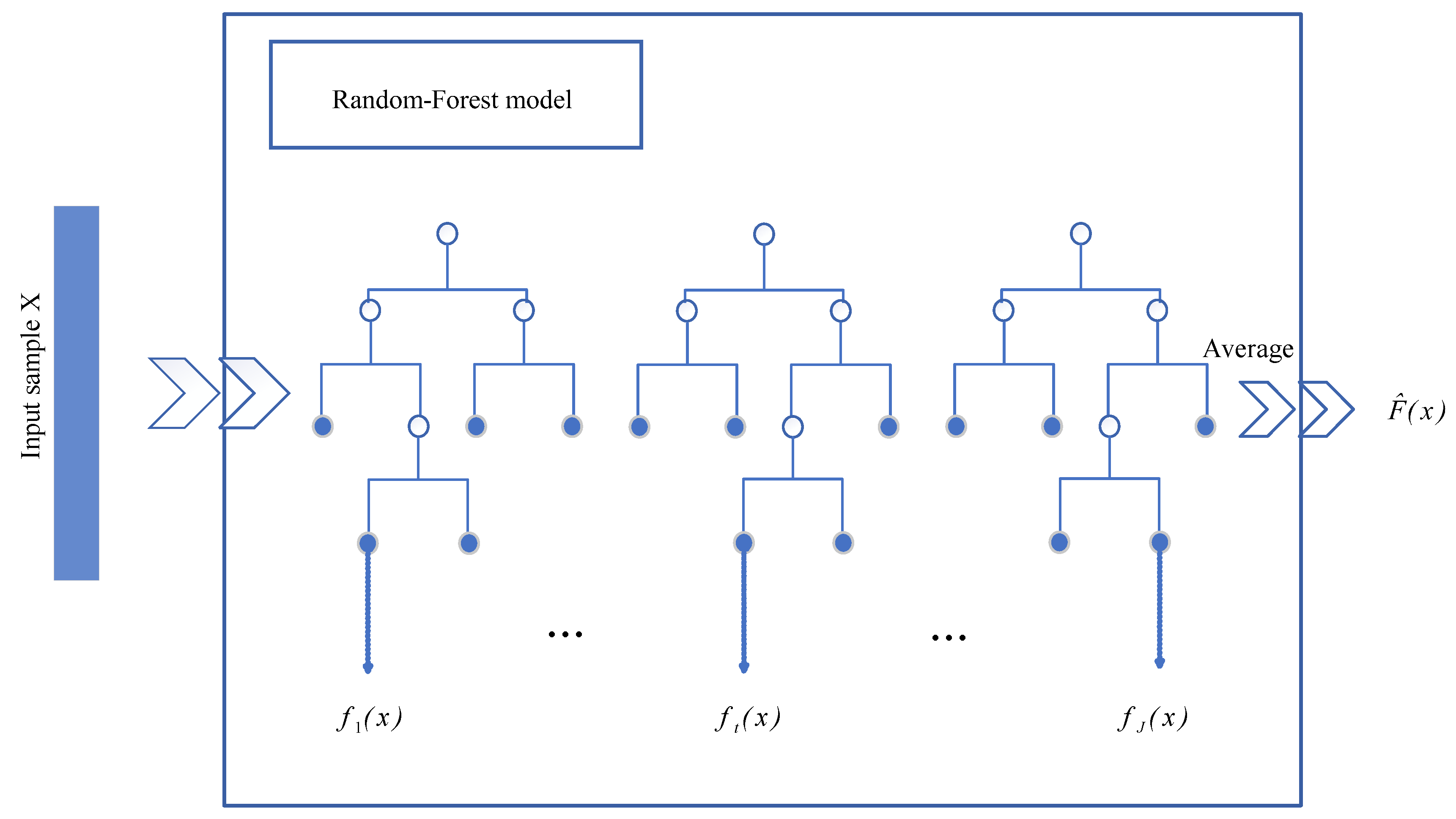
4.1. Random Forest Algorithm

The decision tree (DT) regression algorithm, which consists of a root node, internal nodes, and edges connecting the nodes, is the basis of the random forest algorithm. It is usually divided into three parts: feature selection, tree construction, and pruning. The recursive generation of binomial regression trees by the squared error minimization criterion is briefly described below.

(1)

Specify the training set as $D=\left\{\left(x_1,y_1\right),\left(x_2,y_2\right),\cdots ,\left(x_n,y_n\right)\right\}\in {\mathrm{R}}^{N\times M}$, where N represents the number of samples and M represents the number of feature dimensions. The minimal loss function is defined as follows.

$$\min [{\displaystyle \sum _{x_i\in {\mathrm{R}}_1(j,\mathrm{z})}{\left(y_i-c_1\right)}^2}+{\displaystyle \sum _{x_i\in {\mathrm{R}}_2(j,\mathrm{z})}{\left(y_j-c_2\right)}^2}]$$

(1)

$$\left\{\begin{array}{l}{\mathrm{R}}_1(j,z)=\left\{\left.x\right|x^j\le z\right\}\\ {\mathrm{R}}_2(j,z)=\left\{\left.x\right|x^j>z\right\}\end{array}\right.$$

(2)

(2)

Iterate through each segmentation node j and the segmentation value z of each node. Select the segmentation point by calculating the minimal damage function to divide the sample space into R₁ and R₂. c₁ and c₂ are the corresponding output values of R₁ and R₂ spaces.

(3)

Find the partition point again until it is impossible to continue to divide the subspace.

(4)

The sample space is lastly divided into M parts, and the model can be represented as $f(x)=c_{m}I,x\in {\mathrm{R}}^M$ ; I is taken as 1 when $x\in {\mathrm{R}}^M$.

RF regression is a nonparametric regression method consisting of a set of regression trees $\left\{f_1(x),f_2(x),\cdots ,f_j(x)\right\}$, and this integration obtains the final output by calculating the average of all tree predictions. The procedure is shown in Figure 2 and described in detail as follows:

(1)

J training sets of same size are extracted by the bagging method (BM) and treated as inputs of the tree model. M features are randomly selected as candidate features to participate in the traversal when the tree model is split. Then, J independent regression trees are born.

(2)

Allow each regression tree to grow to its maximal height without pruning.

(3)

The average value of all samples falling on each leaf node is used as the prediction value of the leaf node, and Step (2) is repeated to finish building the J-tree regression tree.

(4)

The RF regression algorithm integrates J regression trees and can be represented as:

$$F(x)=\frac{1}{J}{\displaystyle \sum _{i=1}^J{f}_i}(x)$$

(3)

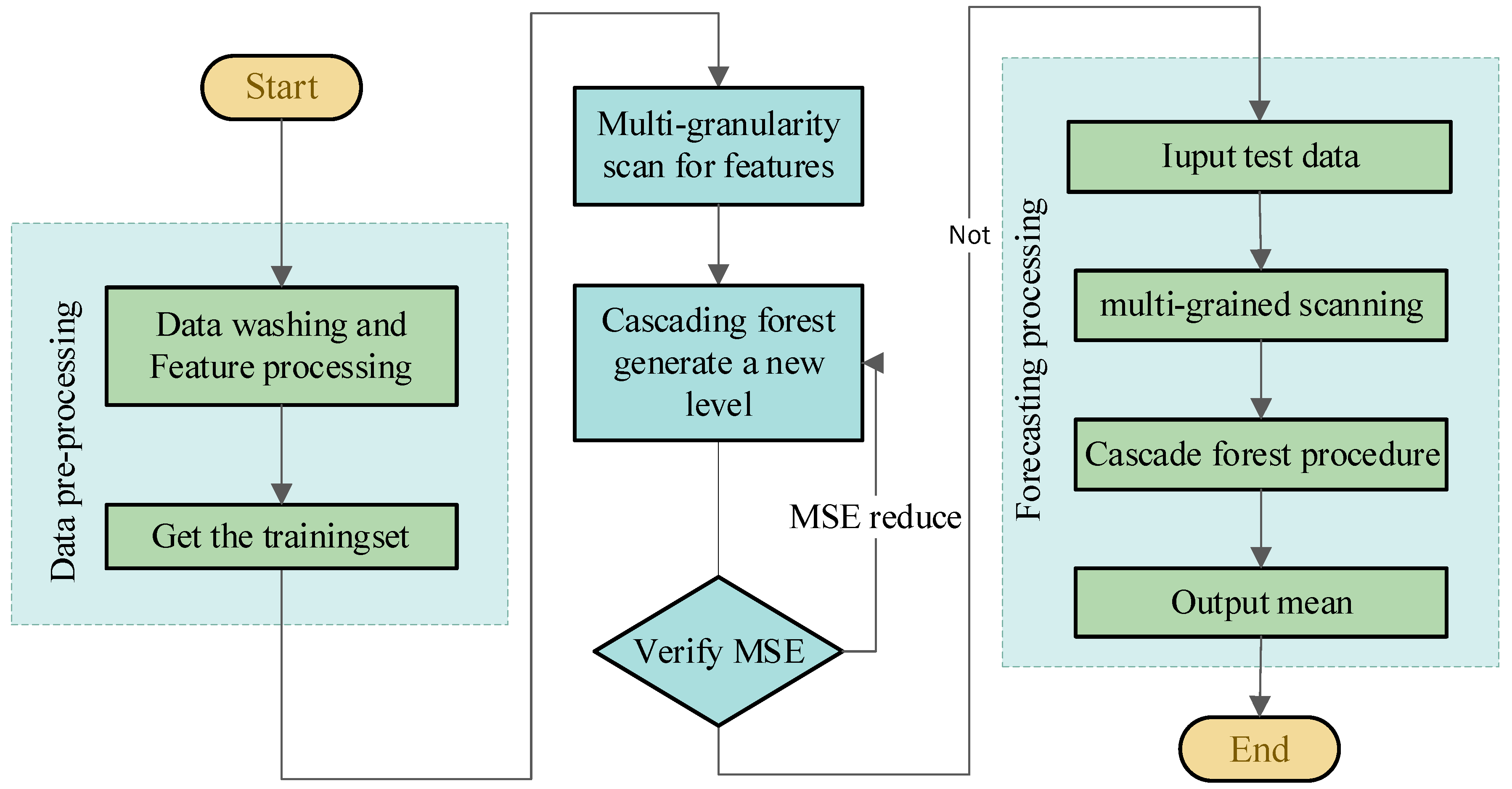
4.2. Deep Forest Algorithm

The integrated deep forest was proposed by Zhou and Feng [23] to solve the complex hyperparameters of deep neural networks (DNNs) through drawing on the successful factors of DNN. The deep forest (DF) model is insensitive to hyperparameters, and achieves better performance on small and medium data. It inherits the DNN’s layer-by-layer stacking structure and can generate new features in the model through which the training set information can be fully utilized.

The prediction process can be divided into multigranularity scanning and cascaded forest [24]. Multigranularity scanning can be designed to map the sample data from a low- to a high-dimensional space by using a sliding-window tool, which aims to fully extract feature information from the training samples. Cascaded forest is inspired by the representation learning approach in DNN, where each cascade structure receives the feature information processed by its previous layer and passes its results to the next layer, adaptively adjusting the number of model layers by validation error.

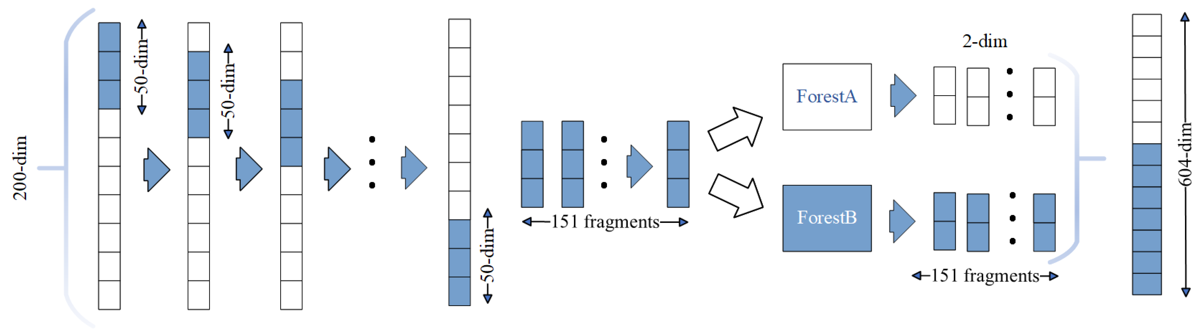
4.2.1. Multigranularity Scanning

The purpose of multigranularity scanning is to convert the original feature vectors into high-dimensional feature vectors, so that the model can overcome the problem of scale variation and fully use the information contained in each sample [25]. Each datum is scanned though multiple granularities to obtain various subsamples. The number of obtained subsamples is calculated with Equation (4).

$$L=(M-h)/\lambda +1$$

(4)

where L represents the number of samples, M is the number of dimension, h is the sliding window length, and $\lambda$ is the sliding step size.

Since the diversity of the integration construct is important for the model’s generalization ability, all acquired vectors were used to train the random forest (Forest A) and the completely random forest (Forest B). The node partitioning of Forest B decision trees is a random selection of all features. Then, each forest training generates a probability vector of length C. L vectors are the input of Forest A (Forest B), and eventually a representation vector of length L * C is produced. For instance, if the 200-dimensional (M = 200) full samples are treated as input, and sliding window length h is set to be 50 with sliding step size $\lambda$ 1, then L = 151, indicating that 151 50-dimensional vectors are generated. Assuming a 2-classification problem, the final synthesis of the base estimators results in a 151 × 2 × 2 dimensional feature vector as the original vector of the cascade forest. Figure 3 shows the whole process of multigranularity scanning.

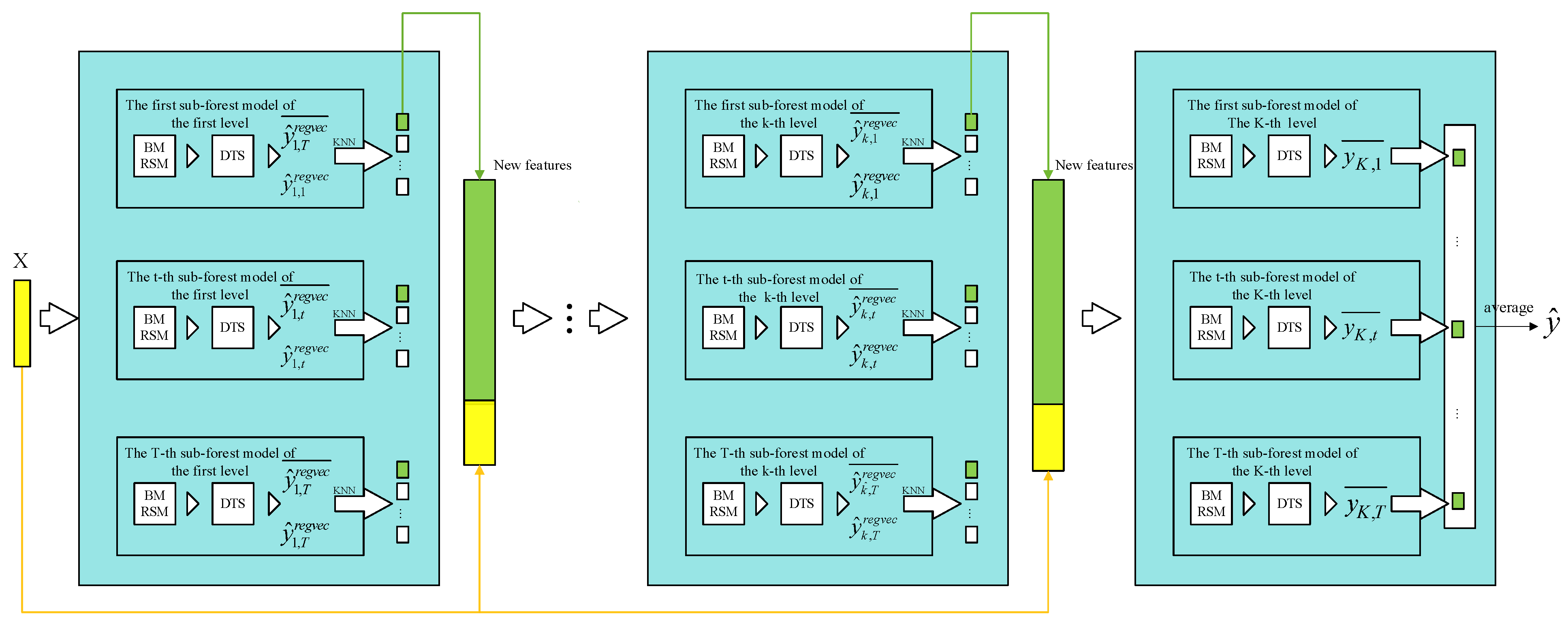
4.2.2. Cascade Forest

In order to fully use the feature information, the random sampling of samples and features through both BM and random subspace method (RSM) was utilized to improve the diversity of training samples for the subforest models [26]. To address the differences between different subforests, two types of forest algorithms, namely, RF and completely random forest (CRF), in the cascade forest structure were used to construct modules for each layer. The two types of forest algorithms have complementary performance between the different submodels, and can improve the overall prediction effectiveness and robustness of the model. Figure 4 shows the process of the cascade forest to process the sample set, with each module consisting of two CRFs and RFs. The flow chart of the deep forest used in this study is shown in Figure 5.

(1)

The transformed feature vectors after multigranularity scanning are used as the original feature vector X at one level in the cascade forest. X through each DTS in the subforest generates the regression vector ${\widehat{y}}_{1,t}^{\mathrm{regvec}}$(where 1 represents the first level of the cascade forest, and t represents the t-th subforest module).

(2)

The adjacent values of the average regression vector ${\overline{\widehat{y}}}_{1,t}^{\mathrm{regvec}}$ are selected by the K-nearest-neighbor method to obtain the augmented layer regression vectors, and then the augmented regression vectors are combined with the initial vectors to obtain new features.

(3)

Using the new features as the input vector of the next level, the output of the second cascade level is obtained in the same way as the input level. The number of born cascade layers is adaptively adjusted by verifying whether mean square error (MSE) decreases. When MSE no longer decreases, the cascade layer stops growing.

(4)

The output layer is the augmented regression vector of the output (K-1)th layer, and the original feature vector is obtained from the multigranularity scanning as input. The final value is the weighted prediction values obtained from the T subforest models in the last layer.

5. Discussion of Results

5.1. Model Evaluation Indicators

Mean square error (MSE), root mean square error (RMSE), mean absolute error (MAE), and correlation coefficient (R²) were used to evaluate the predictive performance of the deep forest and other models. When the values of MSE, RMSE, and MAE are close to 0, it implies better model fitting capability and higher model accuracy. The closer the R² value is to 1, the better the explanatory relationship between the dependent and independent variables is.

$$\mathrm{MSE}=\frac{1}{n}{\displaystyle \sum _{i=1}^n{({\widehat{y}}_i-y_i)}^2}$$

(5)

$$\mathrm{RMSE}=\sqrt{\frac{1}{n}{\displaystyle \sum _{i=1}^n{({\widehat{y}}_i-y_i)}^2}}$$

(6)

$$\mathrm{MAE}=\frac{1}{n}{\displaystyle \sum _{i=1}^n\left|{\widehat{y}}_{\mathrm{i}}-y_{\mathrm{i}}\right|}$$

(7)

$$R^2=1-\frac{{\displaystyle \sum _{i=1}^n{\left({\overline{y}}_i-y_i\right)}^2}}{{\displaystyle \sum _{i=1}^n{\left({\overline{y}}_i-y_i\right)}^2}}$$

(8)

where, ${\widehat{y}}_{\mathrm{i}}$ is the model-predicted value, $y_i$ is the actual value, and ${\overline{y}}_i$ is the mean of the actual value.

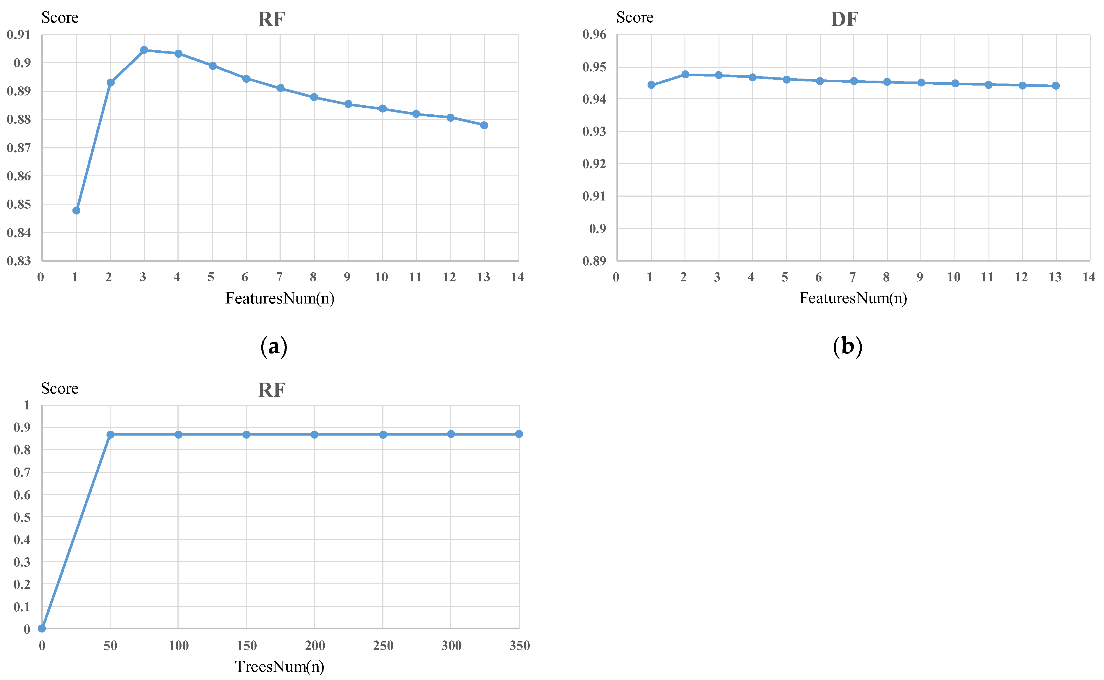
5.2. Forest Model Optimal Parameters

In this study, 75% of the samples were used as the training set, and 25% as the test set. The training set was performed through fivefold cross-validation to obtain more accurate prediction results. The relationships among the number of features, the number of iterations, and score (R²) in the RF and DF models are shown in Figure 6. The R² of RF was the maximal when max_features = 3. Therefore, the number of variables splitting trees in RF was 3. The increase in R² was slower when trees > 250, so that trees = 250. Min_samples_leaf and max_depth had little impact on the model, so they were set to the default values.

Figure 6b shows that the deep forest model is not sensitive to hyperparameters. Thus, the number of trees in each subforest was set to 400. The value of R² reached the peak when max_features = 2. Lastly, for each subforest, max_features = 2, trees = 400, and other parameters were kept as the default values.

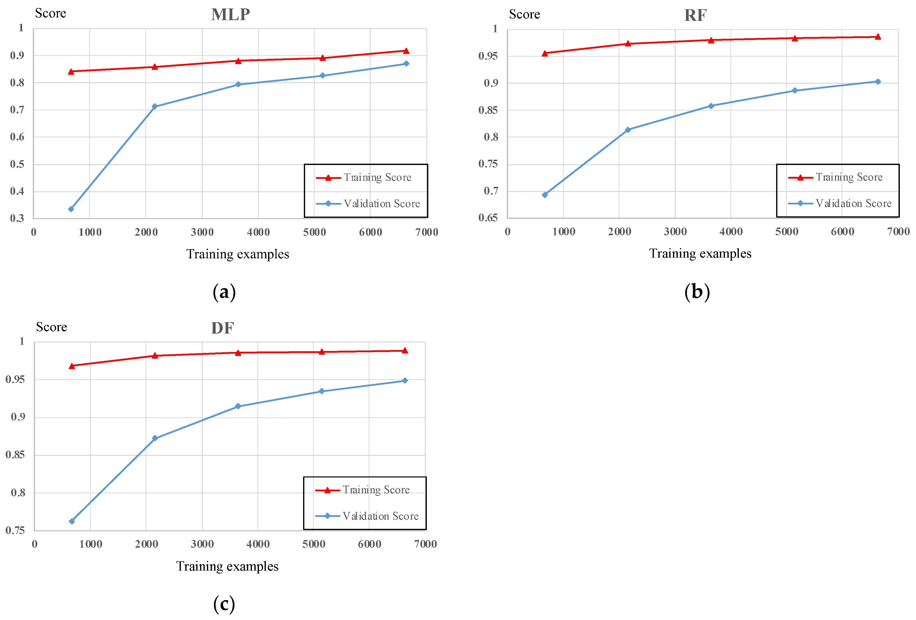
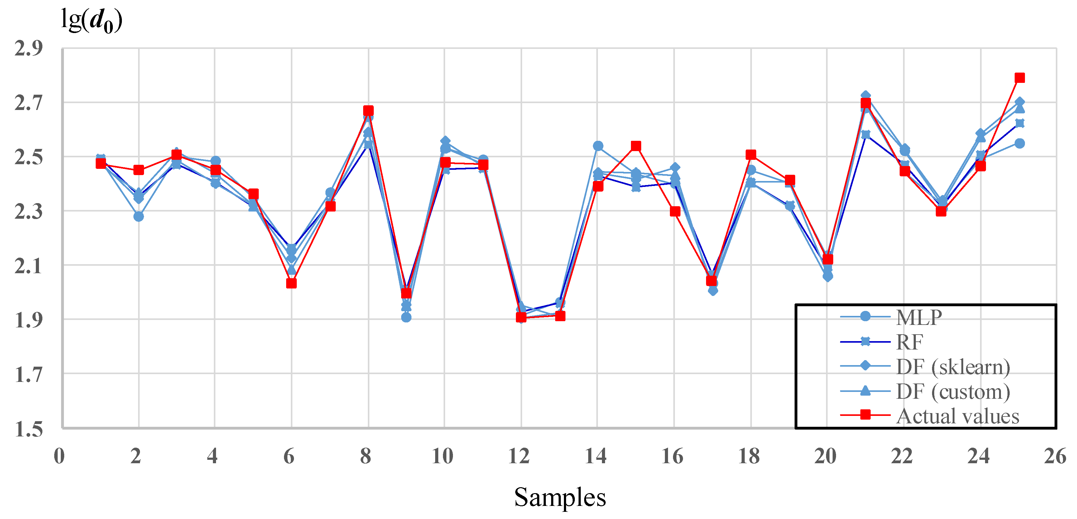
5.3. Method Comparison

On the basis of the same training and test sets, the prediction abilities of MLP, RF, DF (backend: sklearn), and DF (backend: custom) were compared. Different backend programs of DF, including sklearn and custom, have different computational speeds, and the results are different. The corresponding parameters of all models are set as

Table 2. Main parameters of MLP, RF, DF (sklearn), and DF (custom).

Models	Main Parameters	Value
MLP	hidden_layer_size	(92, 46)
	solver	‘relu’
	activation	‘adam’
RF	n_estimatores	250
	max_features	3
DF (sklearn)	n_trees	400
	Max_features	2
DF (custom)	n_trees	400
	max_features	2

.

The learning curves of different models are shown in Figure 7. All curves increased as the number of training examples increased. Among the three methods, the gap of the learning curves between the training and validation sets of MLP was the smallest. The performance of random forest in the training set was much better than that of MLP. The performance of deep forest was as good as that of random forest, and the gap between learning curves was narrow.

The predictive performance of different models is shown in

Table 3. Predictive performance of MLP, RF, DF (sklearn) and DF (custom).

Model	R2	Adjusted R2	MAE	MSE	RMSE	Time	Layer
MLP	0.939	0.908	0.062	0.007	0.082
RF	0.988	0.917	0.060	0.006	0.079
DF (sklearn)	0.992	0.935	0.049	0.005	0.070	4 min 25 s	2
DF (custom)	0.990	0.963	0.038	0.003	0.052	54.3 s	3

. It can be observed that the performance of RF (0.988) in the training set is similar to that of DF (0.990), but the performance of RF in the test set is worse. MLP doesn’t perform as well as RF or DF in the training set, but the performance difference between the test set and training set is slight, which proves MLP had better generalization ability than that of RF in this study. In addition, R² of DF is 0.90 when the training sample is around 3000, which is much better than the RF’s 0.84 and MLP’s 0.76.

The prediction curve of the four models is shown in Figure 8. For Test Samples 2, 9, 14, 22 and 25, MLP’s fitting was poor, and DF could fit the actual value well among the three integrated algorithms because the integrated model achieved better performance, and DF performed better than RF. Some characteristics of the above methods are summarized as follows.

• The MSE, RMSE, MAE, and R² of DF (custom) were better than those of other models, indicating that DF could achieve higher accuracy and better stability in this study.
• The performance of DF is close to RF in learning feature characteristics, but the generalization ability is significantly better than that of RF. MLP’s performance in the training set is significantly inferior to DF and RF, but the generalization capability is good.
• Compared with the highly encapsulated DF (sklearn) model, DF (custom) has certain advantages in terms of computation time and accuracy.

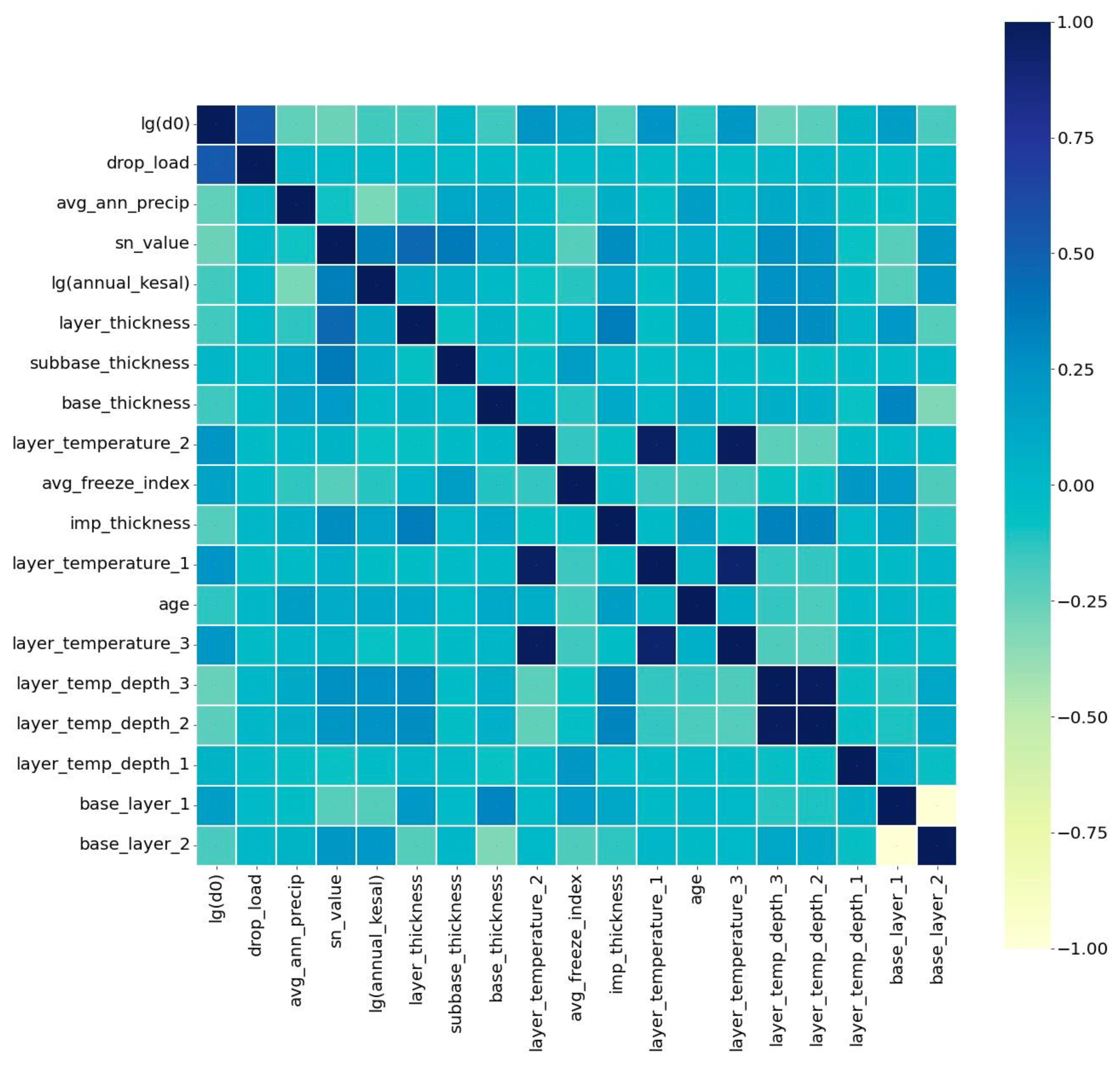
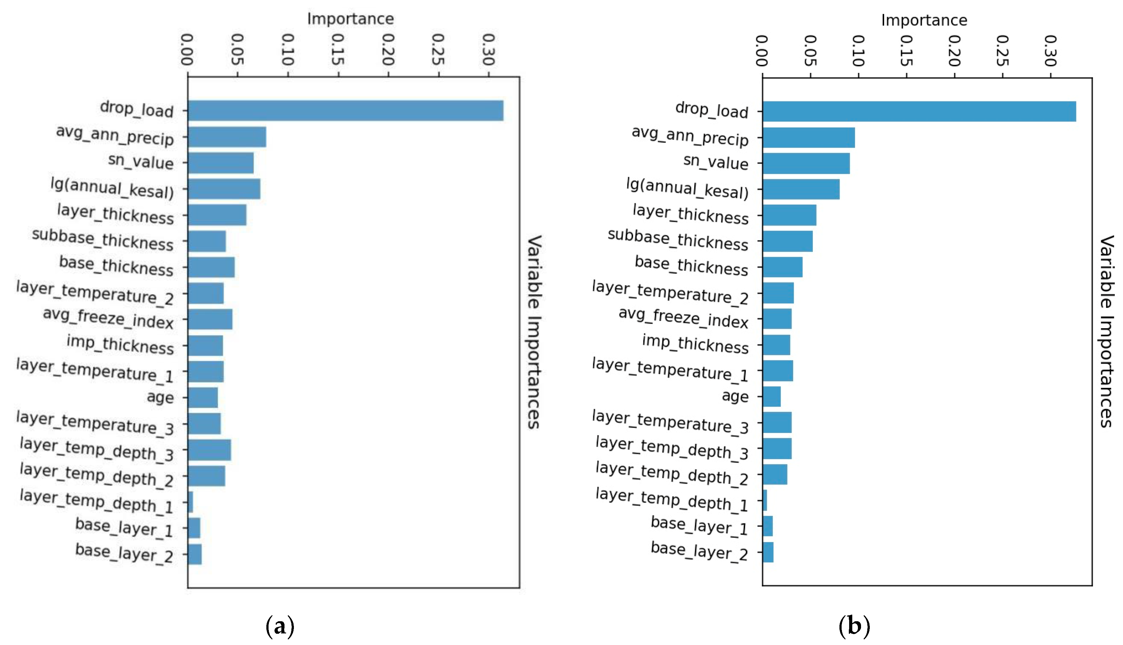
5.4. DF (sklearn) and RF Feature Importance Analysis

In mathematical analysis, the merging of several models with similar prediction results produces a better final output than that of an individual model. The feature importance of DF is defined as the average feature importance values of all base estimators in the cascade layer, which renders it more numerically robust compared to RF. Figure 9b shows the importance scores of 18 feature variables in the first level of DF. lg(d₀) was significantly correlated with drop_load because pavement deformation was directly caused by each load. The average annual traffic volume and average annual precipitation significantly impact central deflection, which is consistent with previous research that greater precipitation and traffic can increase the deflection measurement. The importance of features (sn_value, layer_ thickness, layer_depth, base_thickness, subbase_thickness, and base_layer) related with the pavement structure cannot be ignored. The feature importance of rehabilitation improvement thickness imp_thickness is less than drop_load, avg_ann_precip, sn_value, annual_kesal, avg_freeze_index, and layer_thickness. The layer temperature and pavement age are also related with pavement deflections.

6. Conclusions and Future Work

FWD deflection is an important pavement measurement that can represent a pavement’s structural ability. FWD measurement is related with many influencing factors. In this paper, a new method, DF, was proposed to predict FWD deflection using information related to pavement structures, and traffic and climatic conditions in the LTPP dataset. The regularized MLP, RF, the custom DF model, and the DF model built on the basis of the sklearn backend were used to evaluate and predict pavement deflection.

The results of this study show that all four deep-learning algorithms could identify the complex relationship between FWD deflection lg(d₀) and relevant feature variables with high accuracy and stability. Compared with MLP and RF, the learning and generalization ability of DF was stronger, with MSE, RMSE, MAE and R² better than other models. Between the two deep forest methods, the prediction effect and training time of DF (custom) were better than those of DF (sklearn), indicating that the custom model was superior to the highly encapsulated model with sklearn as the backend. Feature importance analysis in the DF model indicated that drop_load was the key factor affecting lg(d₀). In addition, avg_ann_precip, annual_kesal, and sn_value were very important features related with deflection. Pavement layer thickness, layer depth, and layer temperature were not negligible for the deflection. The feature importance of rehabilitation improvement thickness imp_thickness was less than that of drop_load, avg_ann_precip, sn_value, annual_kesal, avg_freeze_index, and layer_thickness.

In this study, the hyperparameters of machine-learning algorithms were manually tuned. In our future work, the machine-learning methods combined can be used with the optimization algorithms for automatic hyperparameter tuning. In addition, the backcalculation of pavement layer moduli through deep learning will be investigated.

References

1. Mabrouk, G.M.; Elbagalati, O.S.; Dessouky, S.; Fuentes, L.; Walubita, L.F. Using ANN modeling for pavement layer moduli backcalculation as a function of traffic speed deflections. Constr. Build. Mater. 2021, 315, 125736. [Google Scholar] [CrossRef]
2. Han, C.; Ma, T.; Chen, S.; Fan, J. Application of a hybrid neural network structure for FWD backcalculation based on LTPP database. Int. J. Pavement Eng. 2021, 1–14. [Google Scholar] [CrossRef]
3. Plati, C.; Loizos, A.; Gkyrtis, K. Integration of non-destructive testing methods to assess asphalt pavement thickness. NDT E Int. 2020, 115, 102292. [Google Scholar] [CrossRef]
4. Cao, M.; Huang, W.; Zou, Y.; Liu, G. Modulus Inversion Layer by Layer of Different Asphalt Pavement Structures. Adv. Civ. Eng. 2021, 2021, 1–10. [Google Scholar] [CrossRef]
5. Elshaer, M.; Ghayoomi, M.; Daniel, J.S. The role of predictive models for resilient modulus of unbound materials in pavement FWD-deflection assessment. Road Mater. Pavement Des. 2020, 21, 374–392. [Google Scholar] [CrossRef]
6. Muslim, H.B.; Haider, S.W.; Chatti, K. Influence of seasonal and diurnal FWD measurements on deflection-based parameters for rigid pavements. Int. J. Pavement Eng. 2021, 1–12. [Google Scholar] [CrossRef]
7. Zheng, Y.; Zhang, P.; Liu, H. Correlation between pavement temperature and deflection basin form factors of asphalt pavement. Int. J. Pavement Eng. 2019, 20, 874–883. [Google Scholar] [CrossRef]
8. Sollazzo, G.; Fwa, T.; Bosurgi, G. An ANN model to correlate roughness and structural performance in asphalt pavements. Constr. Build. Mater. 2017, 134, 684–693. [Google Scholar] [CrossRef]
9. Gong, H.; Sun, Y.; Shu, X.; Huang, B. Use of random forests regression for predicting IRI of asphalt pavements. Constr. Build. Mater. 2018, 189, 890–897. [Google Scholar] [CrossRef]
10. Gong, H.; Sun, Y.; Dong, Y.; Han, B.; Polaczyk, P.; Hu, W.; Huang, B. Improved estimation of dynamic modulus for hot mix asphalt using deep learning. Constr. Build. Mater. 2020, 263, 119912. [Google Scholar] [CrossRef]
11. Karballaeezadeh, N.; Mohammadzadeh, S.D.; Moazemi, D.; Band, S.S.; Mosavi, A.; Reuter, U. Smart Structural Health Monitoring of Flexible Pavements Using Machine Learning Methods. Coatings 2020, 10, 1100. [Google Scholar] [CrossRef]
12. Barua, L.; Zou, B.; Noruzoliaee, M.; Derrible, S. A gradient boosting approach to understanding airport runway and taxiway pavement deterioration. Int. J. Pavement Eng. 2021, 22, 1673–1687. [Google Scholar] [CrossRef]
13. Guo, R.; Fu, D.; Sollazzo, G. An ensemble learning model for asphalt pavement performance prediction based on gradient boosting decision tree. Int. J. Pavement Eng. 2021, 1–14. [Google Scholar] [CrossRef]
14. Issa, A.; Sammaneh, H.; Abaza, K. Modeling Pavement Condition Index Using Cascade Architecture: Classical and Neural Network Methods. Iran. J. Sci. Technol. Trans. Civ. Eng. 2021, 46, 483–495. [Google Scholar] [CrossRef]
15. Majidifard, H.; Adu-Gyamfi, Y.; Buttlar, W.G. Deep machine learning approach to develop a new asphalt pavement condition index. Constr. Build. Mater. 2020, 247, 118513. [Google Scholar] [CrossRef]
16. Ziari, H.; Maghrebi, M.; Ayoubinejad, J.; Waller, T. Prediction of Pavement Performance: Application of Support Vector Regression with Different Kernels. Transp. Res. Rec. J. Transp. Res. Board 2016, 2589, 135–145. [Google Scholar] [CrossRef]
17. Todkar, S.S.; Le Bastard, C.; Baltazart, V.; Ihamouten, A.; Dérobert, X. Performance assessment of SVM-based classification techniques for the detection of artificial debondings within pavement structures from stepped-frequency A-scan radar data. NDT E Int. 2019, 107, 102128. [Google Scholar] [CrossRef]
18. El-Raof, H.S.A.; El-Hakim, R.A.; El-Badawy, S.M.; Afify, H.A. Simplified Closed-Form Procedure for Network-Level Determination of Pavement Layer Moduli from Falling Weight Deflectometer Data. J. Transp. Eng. Part B Pavements. 2018, 144, 04018052. [Google Scholar] [CrossRef]
19. Karballaeezadeh, N.; Tehrani, H.G.; Shadmehri, D.M.; Shamshirband, S. Estimation of flexible pavement structural capacity using machine learning techniques. Front. Struct. Civ. Eng. 2020, 14, 1083–1096. [Google Scholar] [CrossRef]
20. Bonissone, P.; Cadenas, J.M.; Garrido, M.C.; Díaz-Valladares, R.A. A fuzzy random forest. Int. J. Approx. Reason. 2010, 51, 729–747. [Google Scholar] [CrossRef] [Green Version]
21. Guo, D.; Chen, H.; Tang, L.; Chen, Z.; Samui, P. Assessment of rockburst risk using multivariate adaptive regression splines and deep forest model. Acta Geotech. 2022, 17, 1183–1205. [Google Scholar] [CrossRef]
22. Yin, L.; Sun, Z.; Gao, F.; Liu, H. Deep Forest Regression for Short-Term Load Forecasting of Power Systems. IEEE Access 2020, 8, 49090–49099. [Google Scholar] [CrossRef]
23. Zhou, Z.-H.; Feng, J. Deep forest. arXiv 2017, arXiv:1702.08835. [Google Scholar]
24. Zhou, Z.-H.; Feng, J. Deep forest. National Science Review 2019, 6, 74–86. [Google Scholar] [CrossRef]
25. Yao, Y.; Gu, Y.; Bao, W.; Zhang, L.; Zhu, Y. Golgi Protein Prediction with Deep Forest. In International Conference on Intelligent Computing; Springer: Berlin/Heidelberg, Germany, 2021; pp. 647–653. [Google Scholar]
26. Tang, J.; Xia, H.; Zhang, J.; Qiao, J.; Yu, W. Deep forest regression based on cross-layer full connection. Neural Comput. Appl. 2021, 33, 9307–9328. [Google Scholar] [CrossRef]
Figure 1. Pearson’s correlation coefficient of features.
Coatings 12 01057 g001
Figure 2. Diagram of random forest process.
Coatings 12 01057 g002
Figure 3. Diagram of multigranularity scanning process.
Coatings 12 01057 g003
Figure 4. Diagram of cascade forest module structure.
Coatings 12 01057 g004
Figure 5. Flow chart of deep forest model.
Coatings 12 01057 g005
Figure 6. Tuning curves of (a) RF with different feature numbers, (b) DF with different feature numbers, an (c) RF with different tree numbers.
Coatings 12 01057 g006
Figure 7. Learning curves of MLP, RF, and DF. (a) Learning curves of MLP; (b) Learning curves of RF; (c) Learning curves of DF.
Coatings 12 01057 g007
Figure 8. Prediction curves of MLP, RF, DF (sklearn), and DF (custom).
Coatings 12 01057 g008
Figure 9. Feature importance obtained through RF and DF. (a) Feature importance of RF; (b) feature importance of DF level 1.
Coatings 12 01057 g009