Measurements of Carbon Diffusivity and Surface Transfer Coefficient by Electrical Conductivity Relaxation during Carburization: Experimental Design by Theoretical Analysis

Abstract

The diffusion coefficient (D) and surface transfer coefficient (β) of carbon are important parameters governing the kinetics of carburization, and some other heat treatment processes accompanied by redistribution of carbon in steel. Here, we propose to use an electrical conductivity relaxation (ECR) method for the in situ measurement of D and β of carbon. The feasibility of the method is discussed by the theoretical modeling of carburization for an infinitely long rectangular sample. The synthetic ECR data for the carburization is simulated by tracking the relaxation of electrical conductivity upon a sharp or a gradual change of carbon potential. Then, by Fourier transform, the synthetic ECR data is transformed to an impedance spectroscopy, which is used for estimation of D and β by fitting with a one-dimensional equivalent circuit model. The effects of the width-to-thickness ratio of the sample and the duration of carbon potential buildup on the accuracy of the estimated D and β are studied. The feasibility of the ECR method is verified, and rational guidance for experimental design is proposed.

1. Introduction

Thermochemical treatments, such as carburization can significantly improve the surface properties of metallic materials by diffusion of alloying elements into the surface layer. Among the carburization technologies, gas carburization is a versatile and widely used technology with well-controlled gas composition and temperature. It is recognized that the carburizing process can be divided into three steps: (1) the reactions in gas phase for the build-up of carbon potential; (2) the reactions on steel/gas interface for the transfer of carbon; and (3) the diffusion of carbon into the bulk of steel [1]. A rational design of the carburizing process depends on both the equilibrium thermodynamic parameters (e.g., carbon potential and temperature), and the kinetic parameters (e.g., durations of heating, holding, and cooling, and the flow rates of gases). The thermal equilibrium parameters can be monitored and controlled by the maturely developed probes for O₂, H₂O, and CO₂, and thermal couples, while the kinetic parameters should be designed based on the properties of the steels and the interactions on the steel/gas interface. By linear non-equilibrium thermodynamics, the kinetics of carburizing is governing by the so-called duration of carbon potential build-up (τ_CP, s), the surface transfer coefficient of carbon (β, cm·s⁻¹), and the bulk diffusion coefficient of carbon (D, cm²·s⁻¹). It is usually pre-assumed that the build-up of carbon potential is relatively fast by rational design of convective flow of gases, while the surface transfer and bulk diffusion of carbon are considered as the rate-limiting steps [2,3,4,5,6]. Therefore, β and D are vital to the rational design of carburizing process of specific steels.

From the textbook knowledge [7], the evolution of carbon concentration C(x,t) during carburizing can be descripted based on Fick’s diffusion law by assuming constant values of β and D. This solution has been verified by experimental data. For example, Yan et al. [8] used the analytical solution of Fick’s second law to simulate the carbon concentration distribution of 20 steel with constant diffusion coefficient which was carburized for 4 h at 920 °C and 1 wt.% carbon potential. The simulation results were in general agreement with the experimental results. Some studies show that the C(x,t) can become non-Fickian if β and/or D changes with carbon content and stress. For example, Peng et al. [9] used Fick’s first law with composition-dependent diffusivity to simulate the carbon-content profile of AISI 316L carburized at 743 K and the simulation results matched the experimental results. Christiansen et al. [10] calculated the diffusion coefficient for stress effects in the form of a system wherein diffusion occurs under self-induced chemical stress. To simulate the diffusion profiles, they combined the equations for stress-influenced diffusion into a numerical finite-difference model that handled concentration-dependent diffusion coefficients and incorporated the equilibrium solubility product K, determining the concentration for the onset of precipitation or the trapping of solute atoms. The carbon concentration distribution of carbon steel at 1127 °C was simulated using this model and the calculated results agreed with the experimental data. The concentration profiles obtained from the simulations by the researchers mentioned above are concave shaped and deviate markedly from the complementary error function profiles obtained from constant diffusion coefficients. Furthermore, during the heat treatment process (e.g., annealing and tempering), the samples will undergo diffusion phase change and carbon atoms will diffuse, causing carbon redistribution that can be predicted to some extent by using the diffusion coefficient of carbon. Liu et al. [11] revealed the effect of annealing and mechanical loading on the redistribution of carbon-depth profiles. Carburized 316L austenitic stainless steel was strained with a four-point bending device and isothermally annealed at the temperature range of 300–500 °C for up to 200 h. The results showed that the carburized layer was thermally stable at 300 °C isothermal annealing up to 200 h. At 400 °C and above, the carbon continued to diffuse inward, leading to an increase in the depth of the carburized layer. While four-point bending during isothermal annealing accelerated the diffusion-controlled redistribution of carbon. The kinetic process of carbon redistribution seemed to be determined by the rate of carbon diffusion in low-carbon austenite, rather than that in high-carbon expanded austenite. Niessen et al. [12] investigated the redistribution of carbon in X4CrNiMo16-5-1 martensitic stainless-steel during tempering at 703 K using in situ synchrotron X-ray diffractometry and atom probe tomography. The experimental results showed that the volume of the martensitic cell decreased continuously during tempering, which was caused exclusively by the biased aggregation of interstitial atoms. Tempering led to a gradual rejection of carbon from the solid solution and a bias mainly at grain boundaries. Till now, a consistent understanding of how the values of β and D correlate to the carbon content and stress, and other potential factors, have not been recognized. Probably the most important issue is how the values of β and D can be measured properly.

The commonly used methods for measuring the values of β and D include the weighing method by in situ thermogravimetric measurement or ex situ weighting after carburizing, and glow discharge spectroscopy (GDS) analysis. For example, Yan et al. [13] measured the surface transfer coefficients β of 20, 20CrMnTi, and 20Cr2Ni4 steels at different carburizing temperatures and carbon potentials by ex situ weighing. The results showed that the value of β increased generally with temperature and carbon potential, and a formula is proposed for modeling this relationship. This method is straightforward but time-consuming and labor-intensive, and it is impossible to avoid errors caused by the heating and cooling operations. Therefore, it has not been applied widely. Somers et al. [14] simulated the thermogravimetric carburization under three different experimental conditions. The results showed that the diffusion coefficients could be obtained by stepwise gaseous carburizing of the iron foils, and the smaller the change of carbon content, the more accurate the diffusion coefficient. Then thermogravimetry was applied to continuously monitor the weight change of thin foils of AISI 316 during carburizing in CO-H₂ gas mixtures at 793 K. The initial rate method in which the diffusion coefficient is proportional to the initial slope in a plot of (M_t/M_∞) vs. (t/l²)^1/2 obtained from experiment was used to determinate the diffusion coefficient, where M_t is the weight at time t, M_∞ is the weight after an infinitely long time, and l is the thickness. The experimental results indicated that the diffusion coefficient of carbon in expanded austenite increased with carbon concentration. Thermogravimetric analysis is limited by the atmospheric tolerance of the instrument and cannot be held in the carburizing atmosphere for long duration. This may be the main reason why this method is currently applied to steel foils under decarburization processes. Gao et al. [15] measured β of AISI 316 in different temperature (910 °C, 930 °C, 950 °C, and 970 °C) and in a mixed atmosphere of natural gas and air at different ratios. The carbon concentration distribution curves of the samples were obtained by GDS. An analytical solution of the mass transfer differential equation was used to fit the carbon concentration curves to obtain the value of β. The experimental results revealed that the surface transfer coefficient increased with increasing temperature and carbon potential. GDS is a non-in situ measurement method. The SIMR method proposed by Bengtson [16] is commonly used to convert elemental intensity versus sputtering time, obtained by GDS, into elemental content versus sputtering depth to obtain the concentration distribution of the sample. However, the crater edge effect [17], argon pressure [18], roughness [17], and other factors all have an effect on the depth resolution, and therefore impacts the concentration distribution. At the same time, the sample is measured after quenching, and the surface of the sample is not flat, which will also affect the depth resolution [19]. Therefore, (β, D) obtained by fitting the concentration distribution curve obtained from the GDS to the corresponding mathematical model typically shows significant errors.

Another method that has potential but has not yet been applied to steel is the so-called electrical conductivity relaxation (ECR). The thermodynamic equilibrium of a steady-state system depends on external parameters (e.g., temperature, pressure, or electric field strength). When an equilibrium system is shifted by external parameters (perturbation signal), the time required to re-establish equilibrium is defined as the relaxation time and the reaction kinetics can be characterized in situ by measuring the change in conductivity inside the system over time (response signal). In the last decade, ECR has been mainly applied to measure in situ the (β, D) of the reaction and diffusion of oxygen in ceramic oxides of ceramic fuel cells, including simple perovskite oxides La_1−xSr_xCo_1−yFe_yO_3−δ, La_1−xSr_xMnO_3−δ, Sm_1−xSr_xCoO_3−δ, and Ba_0.5 Sr_0.5Co_0.8Fe_0.2O_3−δ [20,21,22,23], perovskite-type layered oxides PrBaCo_2−yFe_yO_5+δ and Sr₂Fe_2−yMo_yO_5+δ [24,25], and Ruddlesden–Popper-type oxides such as Nd₂NiO_4+δ [26], and CeO₂-based fluorite-type solid solutions [27], which provide fundamental kinetic parameters for solid-state ionics. Recently, we proposed a model for the in situ measurements of the kinetic parameters of the gas carburizing based on the ECR technique and combined with the electrochemical impedance spectroscopy (EIS) technique [28,29]. The sample can be characterized by the Biot number (Bi), defined as $\mathrm{Bi}=L\beta /D$, which can indicate the mechanism (or rate-limiting step) of carburization. When Bi is much less than 0.1 ($\beta \ll D$), the carburization process is controlled by the surface transfer process, and the surface transfer coefficient β plays a decisive role in the rate. When Bi is much greater than 10 ($\beta \gg D$), the carburization process is controlled by the pure diffusion process, and the bulk diffusion coefficient D is the rate-limiting step. When Bi is about 1, the carburization process is controlled by the mixture of the surface transfer process and the diffusion process. The change of the sample conductivity with time during the thermal diffusion process is used instead of the sample mass change. The conductivity relaxation impedance spectroscopy model is used to determine Bi and the diffusion mechanism. Furthermore, D and β are derived.

However, the above model is established under ideal conditions in which the width and length of the sample are infinite and carbon potential is established instantaneously; whether the model can be used to get accurate (β, D) in practical experiments needs to be discussed. Therefore, the objective of this article is to verify the feasibility of the model to the measurement of (β, D) in realistic experiment. The influence of the sample width-to-thickness ratio and the duration of carbon potential build-up on (β, D) are also discussed in this paper. This can provide some rational guidance for experimental design.

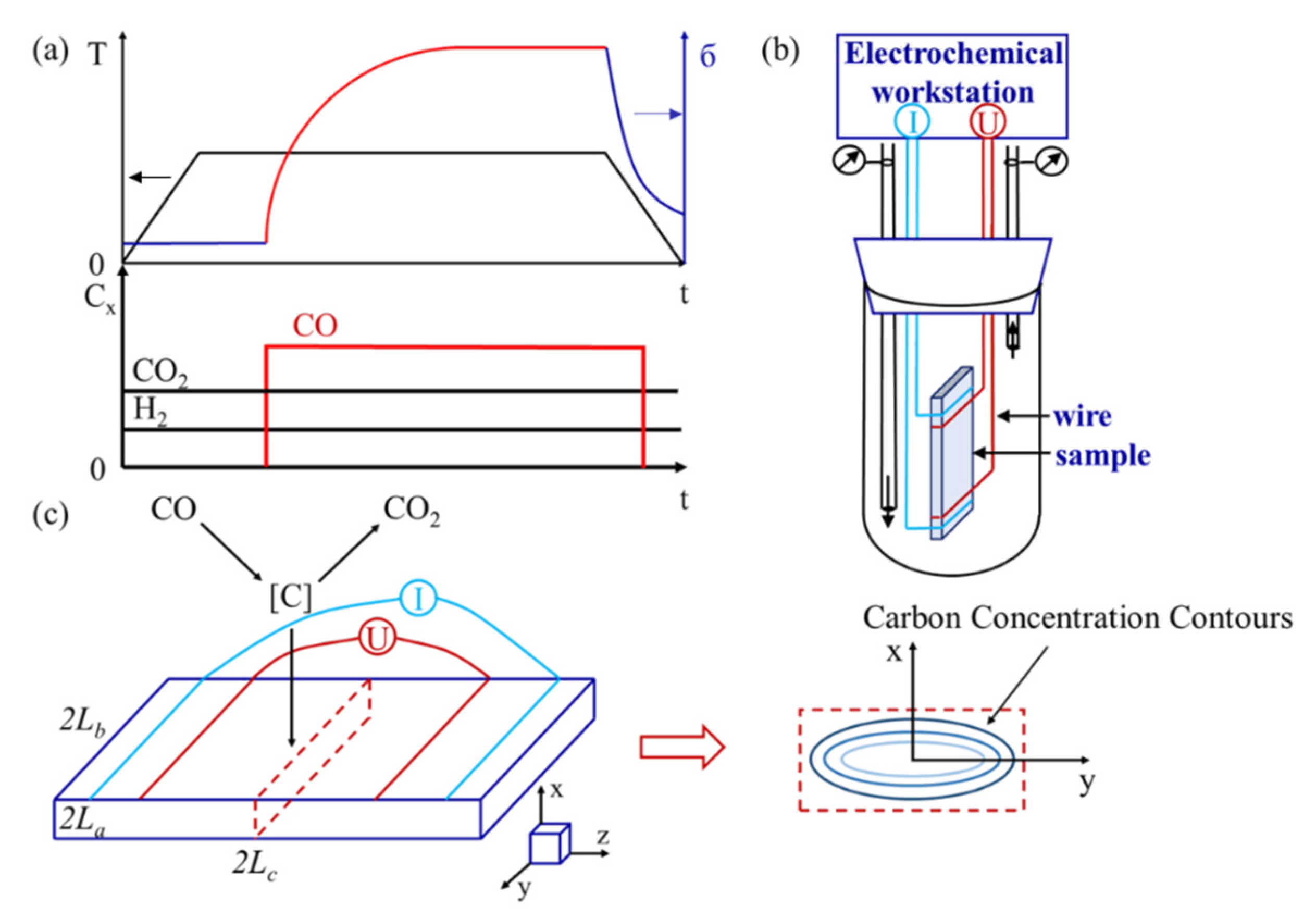
2. Modelling of Gas Carburization

To get (β, D), we design a gas carburization protocol and experimental setup, which can be seen in Figure 1. As shown in Figure 1a, the gas carburization process always keeps the H₂ and CO₂ incoming, and CO is inducted after reaching the carburization temperature. Upon cooling, CO is still applied for a period of time to prevent decarburization of the sample. The red part in б vs. t curve is the data that we may use to obtain (β, D). The experimental setup, which was built by ourselves, is mainly composed of electrochemical workstation, wires, rectangular sample, and inlet and outlet sides. The DC four-terminal method is used to measure the evolution of conductivity with time (Figure 1b). The schematic diagram of the experimental principle is given in Figure 1c. The main reaction of the carburizing atmosphere on the surface of the sample is given by:

$$2CO\rightleftarrows [C]+C{O}_2$$

(1)

The C atoms enter the sample under the driving force. Only the concentration field in the central cross-section of the sample is considered. Due to the long sample, almost all carbon atoms in this cross-section come from the surface of the sample perpendicular to the thickness (x) and width (y) directions. The whole process can be treated as a two-dimensional carburization model.

Due to the small change in carbon potential, it can be considered that the diffusion coefficient D and the surface transfer coefficient β do not change with concentration. In addition, we assume that the diffusion process does not induce phase transformation.

The diffusion process of carbon in the two-dimensional gas carburization model at constant temperature and pressure follows the solution of Fick’s second law under the third type of boundary conditions, given by:

$$\frac{\partial C(x,y,t)}{\partial \mathrm{t}}=D\left(\frac{{\partial }^{2}C(x,y,t)}{\partial x^2}+\frac{{\partial }^{2}C(x,y,t)}{\partial y^2}\right)$$

(2)

with the initial condition:

$$C(x,y,0)=C_0 (-L_a\le x\le L_a,-L_b\le y\le L_b)$$

(3)

and the boundary conditions:

$$-D{\frac{\partial C(x,y,t)}{\partial t}|}_{x=\pm L_a}=\mp \beta [C_{\mathrm{p}}-C(\pm L_a,y,t)] (t>0)$$

(4)

$$-D{\frac{\partial C(x,y,t)}{\partial t}|}_{y=\pm L_b}=\mp \beta [C_{\mathrm{p}}-C(x,\pm L_b,t)] (t>0)$$

(5)

The analytical solution of this model is given in the textbook by Crank J [30].

$$\frac{C\left(x,y,t\right)-C_0}{C_{\mathrm{P}}-C_0}=1-{\displaystyle \sum _{n=1}^{\infty }\times }{\displaystyle \sum _{m=1}^{\infty }\left[\begin{array}{l}\frac{2{\mathrm{Bi}}_x\cos \left(\frac{{\alpha }_{n}x}{L_a}\right)}{{\alpha }_n^2\left({\alpha }_n^2+{\mathrm{Bi}}_x^2+{\mathrm{Bi}}_x\right)}\exp \left(-\frac{{\alpha }_n^{2}Dt}{L_a^2}\right)\\ \times \frac{2{\mathrm{Bi}}_y\cos \left(\frac{{\beta }_{m}y}{L_b}\right)}{{\beta }_m^2\left({\beta }_m^2+{\mathrm{Bi}}_y^2+{\mathrm{Bi}}_y\right)}\exp \left(-\frac{{\beta }_m^{2}Dt}{L_b^2}\right)\end{array}\right]}$$

(6)

$${\alpha }_n\tan ({\alpha }_n)=\mathrm{Bi}=L\frac{\beta }{D}$$

(7)

where α_n is the set of positive roots of Equation (7).

When the C concentration is low and the change is small, the change in conductivity is proportional to the change in carbon content, so the local conductivity can be expressed as:

$$\frac{\sigma \left(x,y,t\right)-\sigma \left(0\right)}{\sigma (\infty )-\sigma \left(0\right)}=1-{\displaystyle \sum _{n=1}^{\infty }\times }{\displaystyle \sum _{m=1}^{\infty }\left[\begin{array}{l}\frac{2{\mathrm{Bi}}_x^2}{{\alpha }_n^2\left({\alpha }_n^2+{\mathrm{Bi}}_x^2+{\mathrm{Bi}}_x\right)}\exp \left(-\frac{{\alpha }_n^{2}Dt}{L_a^2}\right)\\ \times \frac{2{\mathrm{Bi}}_y^2}{{\beta }_m^2\left({\beta }_m^2+{\mathrm{Bi}}_y^2+{\mathrm{Bi}}_y\right)}\exp \left(-\frac{{\beta }_m^{2}Dt}{L_b^2}\right)\end{array}\right]}$$

(8)

As shown in Figure 1b, the DC four-terminal method in the experiment is used to measure the macroscopic conductivity σ_app(t) of the three-dimensional sample. Since the length of the sample in the test is much larger than the thickness and width, the equivalence surface can be considered as perpendicular to the direction between the two voltage probes. Therefore, the total macroscopic conductivity σ_app(t) of the sample can be considered as a series of sheet conductivities σ(x, y, t) along the z-direction:

$${\sigma }_{\mathrm{app}}\left(t\right)=\frac{1}{L_a{L}_b}{\displaystyle {\int }_0^{L_a}{\displaystyle {\int }_0^{L_b}\sigma \left(x,y,t\right)\mathrm{d}x\mathrm{d}y}}$$

(9)

Inserting Equation (9) into Equation (8), the relaxation of the macroscopic conductivity can therefore be expressed in terms of the normalized conductivity as:

$$\overline{\sigma }(t)=\frac{{\sigma }_{\mathrm{app}}\left(t\right)-{\sigma }_{\mathrm{app}}\left(0\right)}{{\sigma }_{\mathrm{app}}(\infty )-{\sigma }_{\mathrm{app}}\left(0\right)}=1-{\displaystyle \sum _{n=1}^{\infty }\times }{\displaystyle \sum _{m=1}^{\infty }\left[\begin{array}{l}\frac{2{\mathrm{Bi}}_x^2}{{\alpha }_n^2\left({\alpha }_n^2+{\mathrm{Bi}}_x^2+{\mathrm{Bi}}_x\right)}\exp \left(-\frac{{\alpha }_n^{2}Dt}{L_a^2}\right)\\ \times \frac{2{\mathrm{Bi}}_y^2}{{\beta }_m^2\left({\beta }_m^2+{\mathrm{Bi}}_y^2+{\mathrm{Bi}}_y\right)}\exp \left(-\frac{{\beta }_m^{2}Dt}{L_b^2}\right)\end{array}\right]}$$

(10)

which gives the normalized conductivity in the ECR.

Ciucci F [31] revealed that it was difficult to obtain accurate (D, β) from the ECR curves alone because of a poor process resolution. In contrast, the EIS technique based on the frequency domain analysis approach has a high process resolution. The kinetic parameters (D, β) of the reaction spreading process can be resolved by fitting the impedance spectrum according to the equivalent circuit model. To obtain the corresponding impedance spectrum, a time-frequency transformation of the ECR data is required, given by:

$$\tilde{\sigma }(\omega )={{\displaystyle {\int }_0^{\infty }\overline{\sigma }(t)\cdot e}}^{-\mathrm{j}\omega t}\mathrm{d}t$$

(11)

Although the Fourier transform represented by Equation (11) is very simple, the expression cannot be used directly because of a discrete set of data points over a limited time range measured by the experiment.

Boukamp [32] proposed a simple linear interpolation method, where a linear interpolation function is constructed between two data points ${\sigma }_i{}_{-1}$ and ${\sigma }_i$, and the approximate integration is achieved by summing the data. The linear interpolation function is given by:

$$\overline{\sigma }\left(t\right)=\frac{{\sigma }_i-{\sigma }_{i-1}}{t_i-t_{i-1}}t+b$$

(12)

Equation (12) is brought into Equation (11) to obtain the Fourier transform of the finite ECR data set.

$$\begin{array}{ll}{{\tilde{\sigma }}^{\prime }(\omega )|}_0^{t_N}=& {\displaystyle \sum _{i=1}^N[X_i\sin }\omega t_i-X_{i-1}\sin \omega t_{i-1}+\frac{a}{\omega }(\cos \omega t_i-\cos \omega t_{i-1})]\cdot {\omega }^{-1}\\ & +j{\displaystyle \sum _{i=1}^N[X_i\cos }\omega t_i-X_{i-1}\cos \omega t_{i-1}+\frac{a}{\omega }(\sin \omega t_i-\sin \omega t_{i-1})]\cdot {\omega }^{-1}\end{array}$$

(13)

In addition, by modeling the end region of the ECR data with the exponential function, the finite conductivity relaxation data can be extrapolated to relaxation equilibrium at time parameter t at infinity.

$$\overline{\sigma }(t)={\sigma }_0+{\sigma }_1\cdot e^{-t/\tau }$$

(14)

The Fourier transform of the ECR from the time parameter t_N corresponding to the last data to t = ∞ is obtained:

$$\begin{array}{ll}{\tilde{\sigma }}^{″}(\omega )|\begin{array}{c}\infty \\ t_N\end{array}=& -\frac{{\sigma }_0}{\omega }\left[\sin \omega t_N+\cos \omega t_N\right]+\\ & +{\sigma }_1{e}^{-\frac{t_N}{\tau }}\{\frac{{\tau }^{-1}\cos \omega t_N-\omega \sin \omega t_N}{{\omega }^2+{\tau }^{-2}}+j\frac{\omega \cos \omega t_N+{\tau }^{-1}\sin \omega t_N}{{\omega }^2+{\tau }^{-2}}\}\end{array}$$

(15)

Combining Equations (13) and (15), the measured ECR data can be converted into the frequency domain.

$$\tilde{\sigma }(\omega )={\tilde{\sigma }}^{\prime }(\omega )|\begin{array}{c}{t}_N\\ 0\end{array}+{\tilde{\sigma }}^{″}(\omega )|\begin{array}{c}\infty \\ t_N\end{array}$$

(16)

EIS data can be obtained from the following equation with the corresponding ECR data from the experiment.

$$Z\left(\omega \right)=-\frac{1}{{\omega }^2\cdot \left(\frac{1}{j\cdot \omega }-\tilde{\sigma }(\omega )\right)}$$

(17)

Although the method can convert ECR data into impedance spectrum, its infinite series solution limits the accuracy of curve fitting because the two-dimensional carburization model does not have an impedance spectrum model with an analytical solution.

Boukamp [32] proposed the analytical solution of the impedance spectrum model for the one-dimensional carburization model. When the width is much larger than the thickness, the two-dimensional carburization model can be simplified to a one-dimensional carburization model. In this case, its normalized conductivity model Equation (10) is simplified as:

$$\overline{\sigma }(t)=1-{\displaystyle \sum _{n=1}^{\infty }\frac{2{\mathrm{Bi}}_x^2}{{\alpha }_n^2\left({\alpha }_n^2+{\mathrm{Bi}}_x^2+{\mathrm{Bi}}_x\right)}\exp \left(-\frac{{\alpha }_n^{2}Dt}{L_a^2}\right)}$$

(18)

According to the definition of impedance, the change in the carbon potential of the atmosphere is taken as the perturbation signal, and carbon flux $J(t)$ at the sample surface is replaced by the experimental measurable signal conductivity, which is the response signal. The expression of the conductivity relaxation impedance spectrum is given by:

$$Z(\omega )=\frac{ℒ\left(\mathsf{\Delta }C(t)\right)}{ℒ\left(J(t)\right)}=\frac{1}{{\omega }^2\cdot \tilde{\sigma }(\omega )}=\frac{L_a}{\beta }+\frac{L_a}{\sqrt{\mathrm{j}\omega D}}\coth L_a\sqrt{\frac{\mathrm{j}\omega }{D}}$$

(19)

where $\tilde{\sigma }(\omega )$ represents the Fourier transform of the ECR response.

The boundary conditions of the carburization model are based on the assumption that the change of the carbon potential is completed instantaneously, which greatly simplifies the mathematical treatment process. However, the sudden change of the carbon potential in the experiment is difficult to achieve, and there is often a relaxation time for the change of the carbon potential, defined as the duration of carbon potential buildup τ_Cp, which is usually shortened as much as possible to minimize its effect on the (β, D) measurement. Therefore, the mathematical model must be corrected for τ_Cp.

The normalized conductivity Equation (10) for two-dimensional carburization is corrected for τ_Cp as [33]:

$$\begin{array}{c}\overline{\sigma }\left(t\right)=1-\exp \left(-\frac{t}{{\tau }_{C_p}}\right)-{\displaystyle \sum _{n=1}^{\infty }{\displaystyle \sum _{m=1}^{\infty }\frac{2{\mathrm{Bi}}_x^2}{{\alpha }_n^2\left({\alpha }_n^2+{\mathrm{Bi}}_x^2+{\mathrm{Bi}}_x\right)}\times \frac{2{\mathrm{Bi}}_y^2}{{\beta }_m^2\left({\beta }_m^2+{\mathrm{Bi}}_y^2+{\mathrm{Bi}}_y\right)}\times \frac{{\tau }_{n,m}}{{\tau }_{n,m}-{\tau }_{C_p}}}}\\ \times \left[\exp \left(-\frac{t}{{\tau }_{n,m}}\right)-\exp \left(-\frac{t}{{\tau }_{C_p}}\right)\right]\end{array}$$

(20)

$${\tau }_{n,m}=\frac{1}{D\times \left[{\left(\frac{{\alpha }_n}{L_a}\right)}^2+{\left(\frac{{\beta }_m}{L_b}\right)}^2\right]}$$

(21)

For the impedance spectrum model of one-dimensional carburization, the perturbed signal $\mathsf{\Delta }C(t)$ is replaced by a continuously varying exponential model.

$${\tilde{C}}_{\mathrm{cor}}(\omega )=\frac{\mathsf{\Delta }C}{j\omega (j\omega {\tau }_{C_p}+1)}$$

(22)

The impedance spectrum model of Equation (19) with the correction of τ_Cp can be obtained as follows:

$$Z^{\prime }(\omega )=(1+\mathrm{j}\omega {\tau }_{C_p})\cdot \left(\frac{L_a}{\beta }+\frac{L_a}{\sqrt{\mathrm{j}\omega D}}\coth L_a\sqrt{\frac{\mathrm{j}\omega }{D}}\right)$$

(23)

3. Result and Discussion

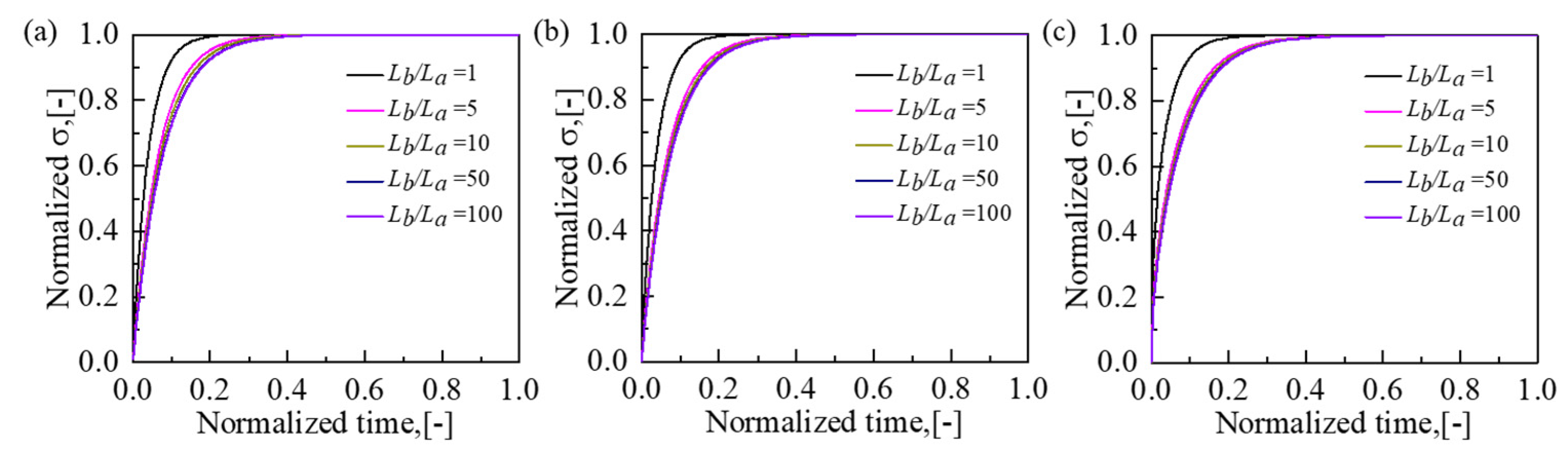
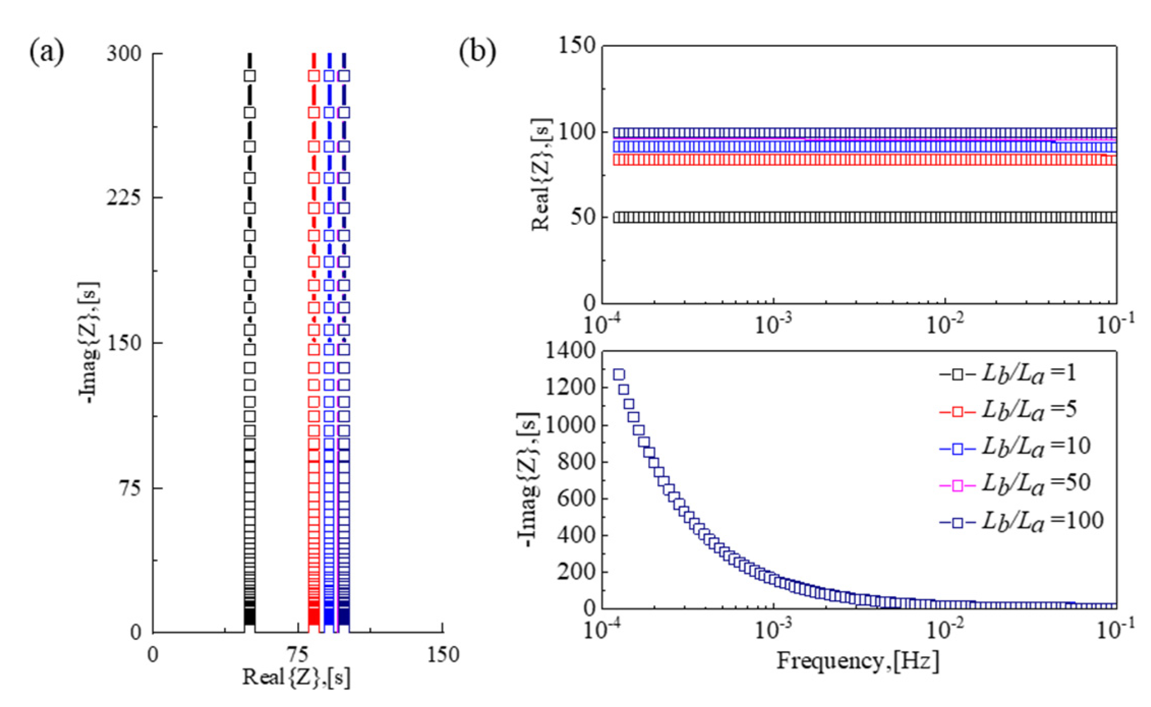
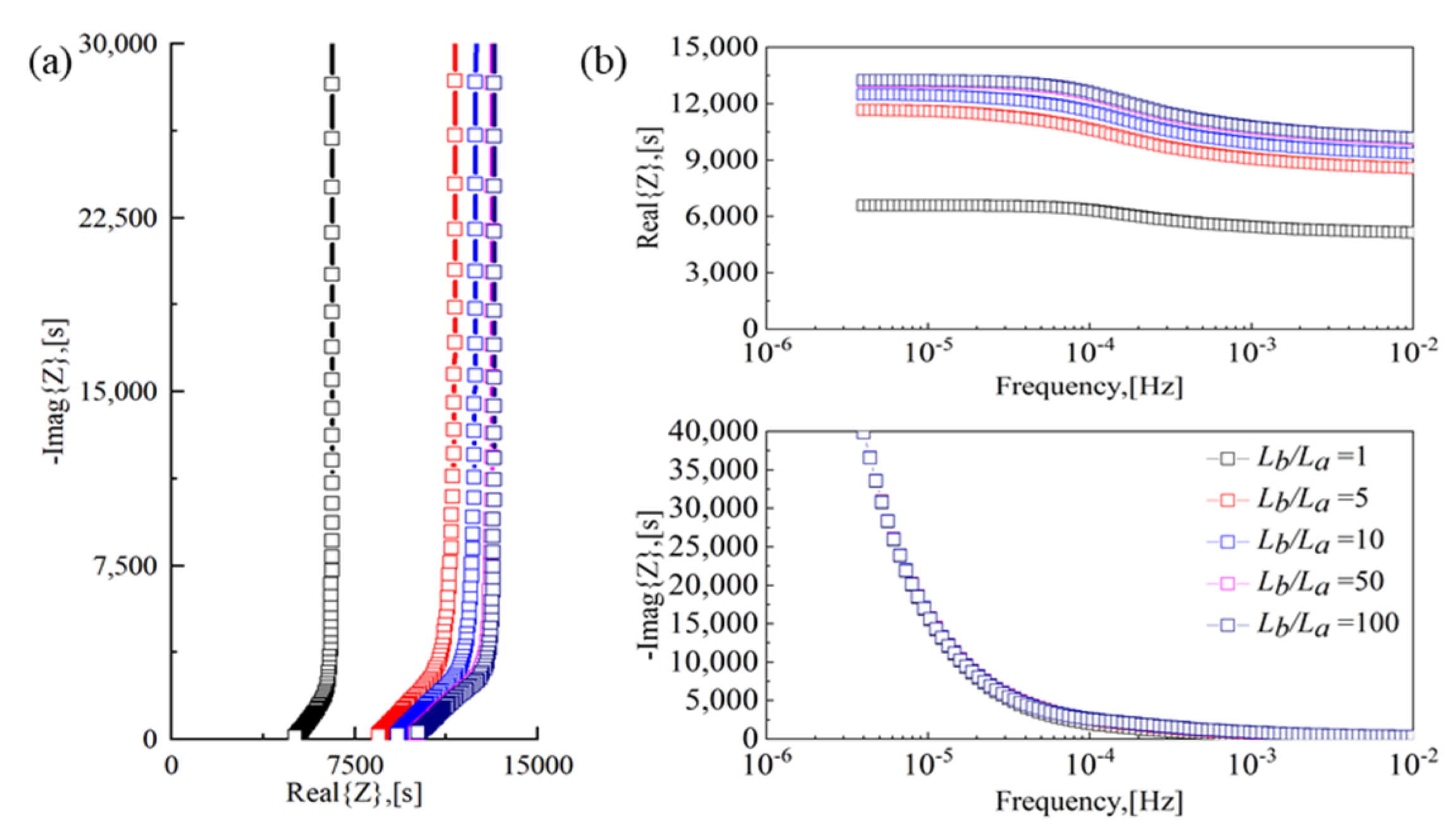
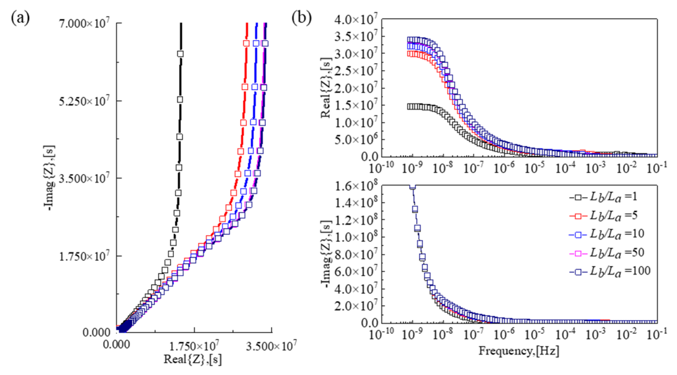
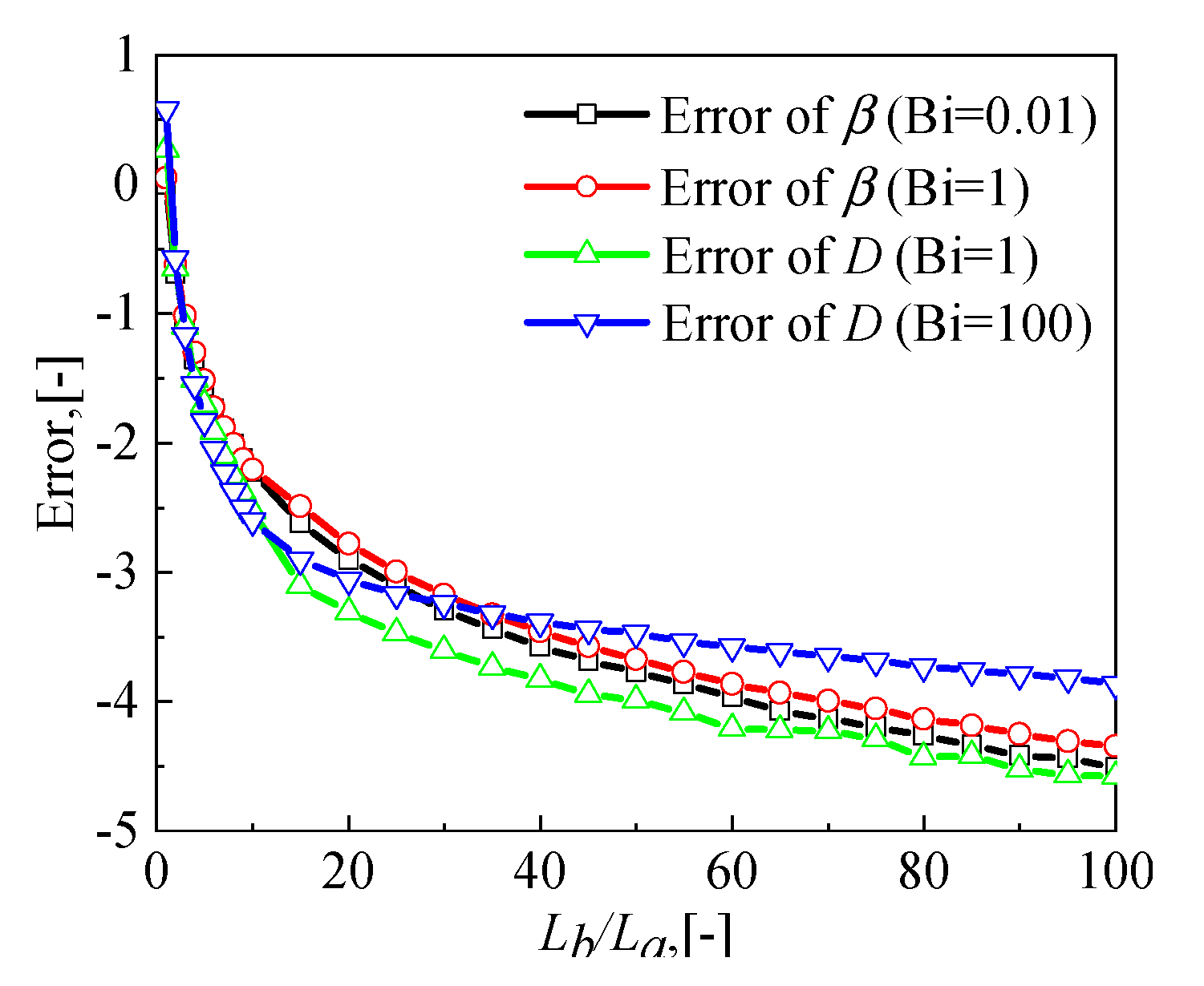
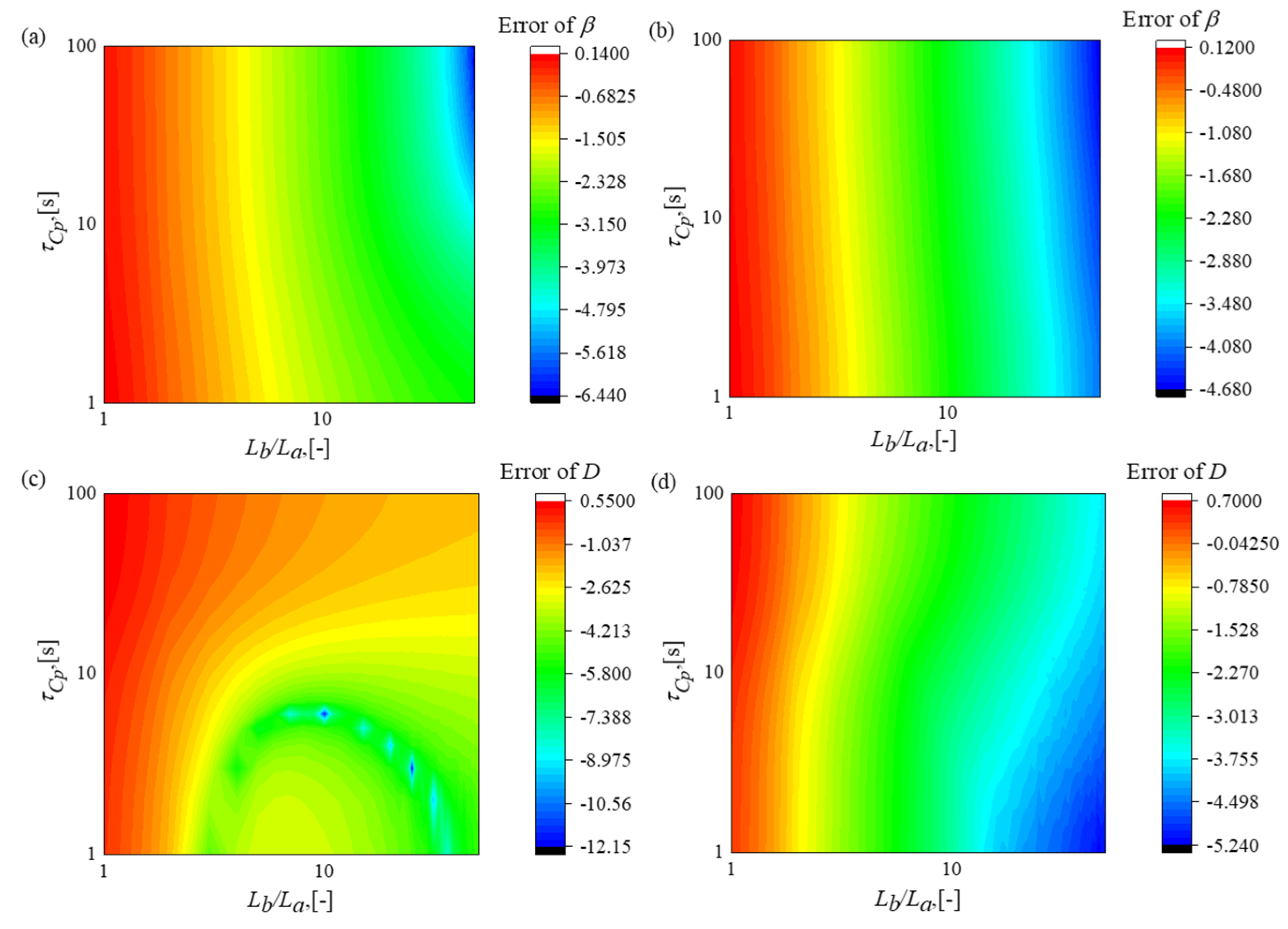
3.1. The Influence of Width-to-Thickness Ratio

(β, D) are considered to be obtained by fitting Equation (23) with EIS data from the experiment. As previously mentioned, Equation (23) is obtained in one-dimensional model, while the width of the sample is finite, which may cause the error of (β, D). Therefore, the influence of width-to-thickness ratio is discussed in this section to get a proper width-to-thickness ratio that is the most suitable to the experiment.

We use Equation (10) to simulate the ECR data from the experiment. The input parameters are shown in

Table 1. Parameters of conductivity relaxation with different Bi.

Bi	τCp (s)	β (cm/s)	D (cm2/s)	La (cm)	Lb (cm)	Lb/La
0.01	0	1 × 10−6	1 × 10−8	1 × 10−4	1 × 10−4~1 × 10−2	1, 5, 10, 50, 100
1				1 × 10−2	1 × 10−2~1
100				1	1~100

. The surface exchange coefficient β, the diffusion coefficient D, the duration of carbon potential buildup τ_Cp, and the sample thickness L_a are constant, and the width-to-thickness ratio of the order of 1 to 100 is changed by changing the sample width L_b. Figure 2a–c show the conductivity relaxation curves of different Bi respectively. Normalized time is given by $\overline{t }{=t/t}_{\max }$. As shown in Figure 2a–c, with the increase in the width-to-thickness ratio, the relaxation time gradually increases because of the longer time required to complete the thermal diffusion with the increase in the sample size. Therefore, it is necessary to consider the influence of the width-to-thickness ratio on thermal diffusion time.

Figure 3 shows the electric impedance spectroscopy of different width-to-thickness ratios obtained by Fourier transforming Bi = 0.01 conductivity relaxation data. As shown in Figure 3a, the change of the width-to-thickness ratio does not affect the characteristics of the impedance spectroscopy, and the Warburg-type diffusion cannot be found, which is a pure capacitive behavior. Therefore, in the fitting of the kinetic parameter, only β is considered. Figure 4 shows the electric impedance spectroscopy of Bi = 1. The characteristic of pure capacitive behavior at low frequency and Warburg-type diffusion at high frequency can be seen in Figure 4a, so both D and β can be obtained by fitting the EIS model. The calculated impedance spectroscopy of Bi = 100 is shown in Figure 5. Warburg-type diffusion can be observed in Figure 5a. The high-frequency part of the impedance spectroscopy will pass through the origin after extrapolation, so an accurate β cannot be derived according to the equation and only D is considered. Since each electric impedance spectroscopy in Figure 3, Figure 4 and Figure 5 has the same characteristics as that obtained by the one-dimensional model, (β, D) can be achieved by fitting Equation (19). Meanwhile, in Figure 3a–5a, curves with width-to-thickness ratios of 50 and 100 nearly overlap, which means (β, D) are similar. The errors of two kinetic parameters (β, D) are shown in Figure 6. The error is given by ${E=\log }_{10}\left(/i_{\mathrm{cal}} {- i}_0/{/i}_0\right)(i=\beta , D)$, where i_cal is a calculated value and i₀ is a given value.

As shown in Figure 6, the errors of β and D decrease gradually with the increase of the width-to-thickness ratio. When the width-to-thickness ratio is relatively small, the error decreases fast, and when it is relatively large, the error declines flatly. Though the error continues to decrease, the relative errors of (β, D) are only about 2% when the width-to-thickness ratio is 50. Therefore, considering the error and carburizing time, the width-thickness ratio of 50 is suitable.

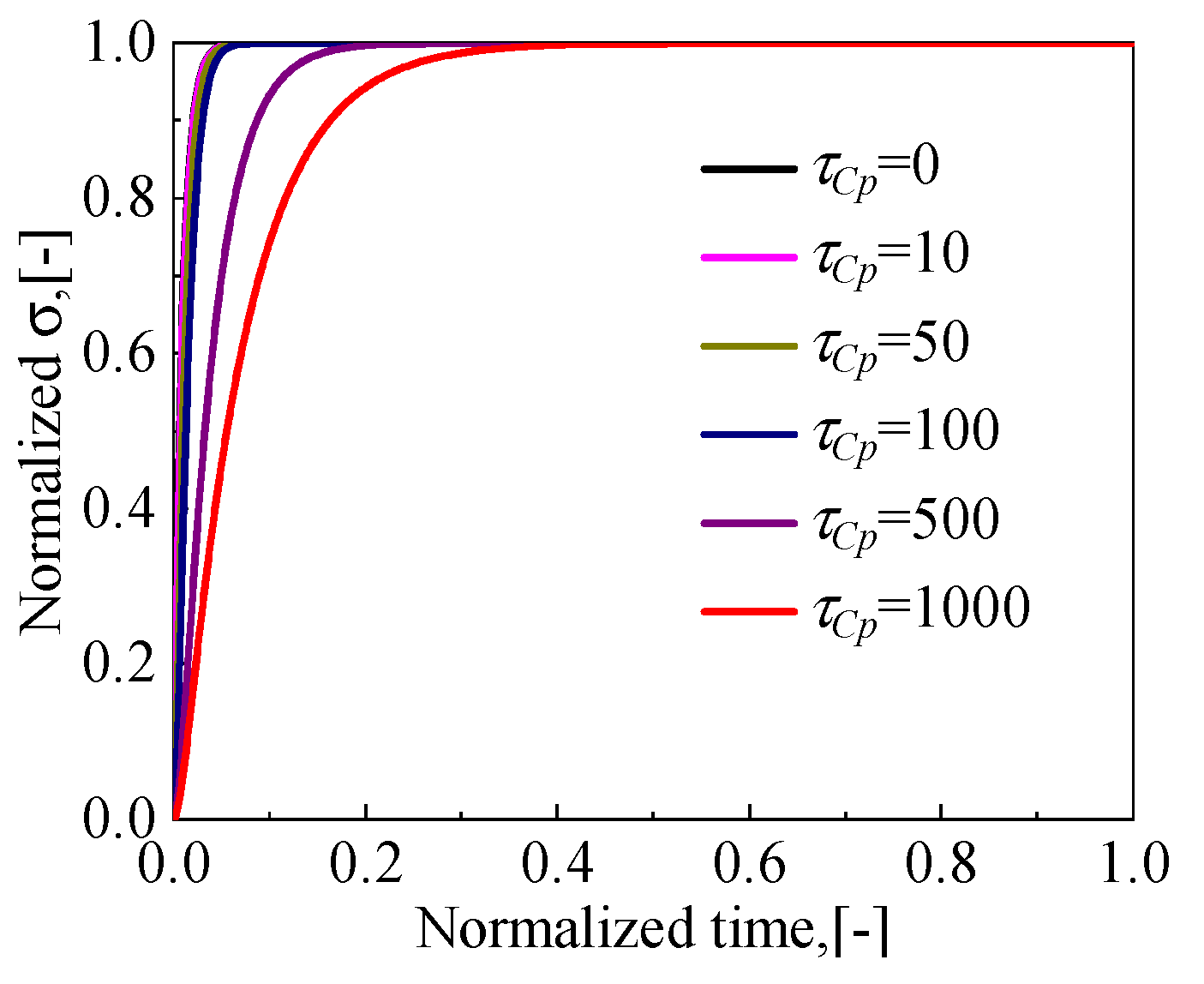
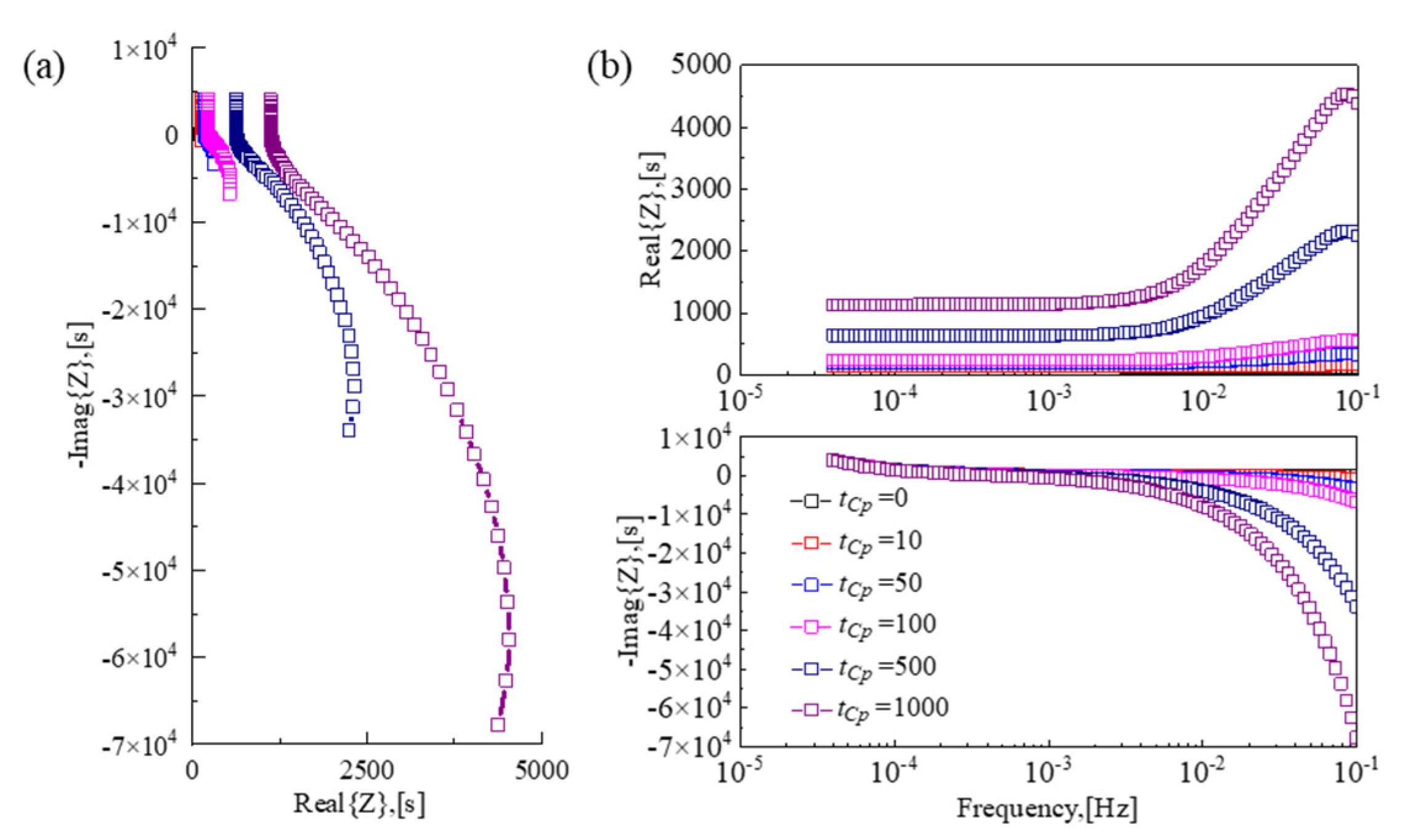
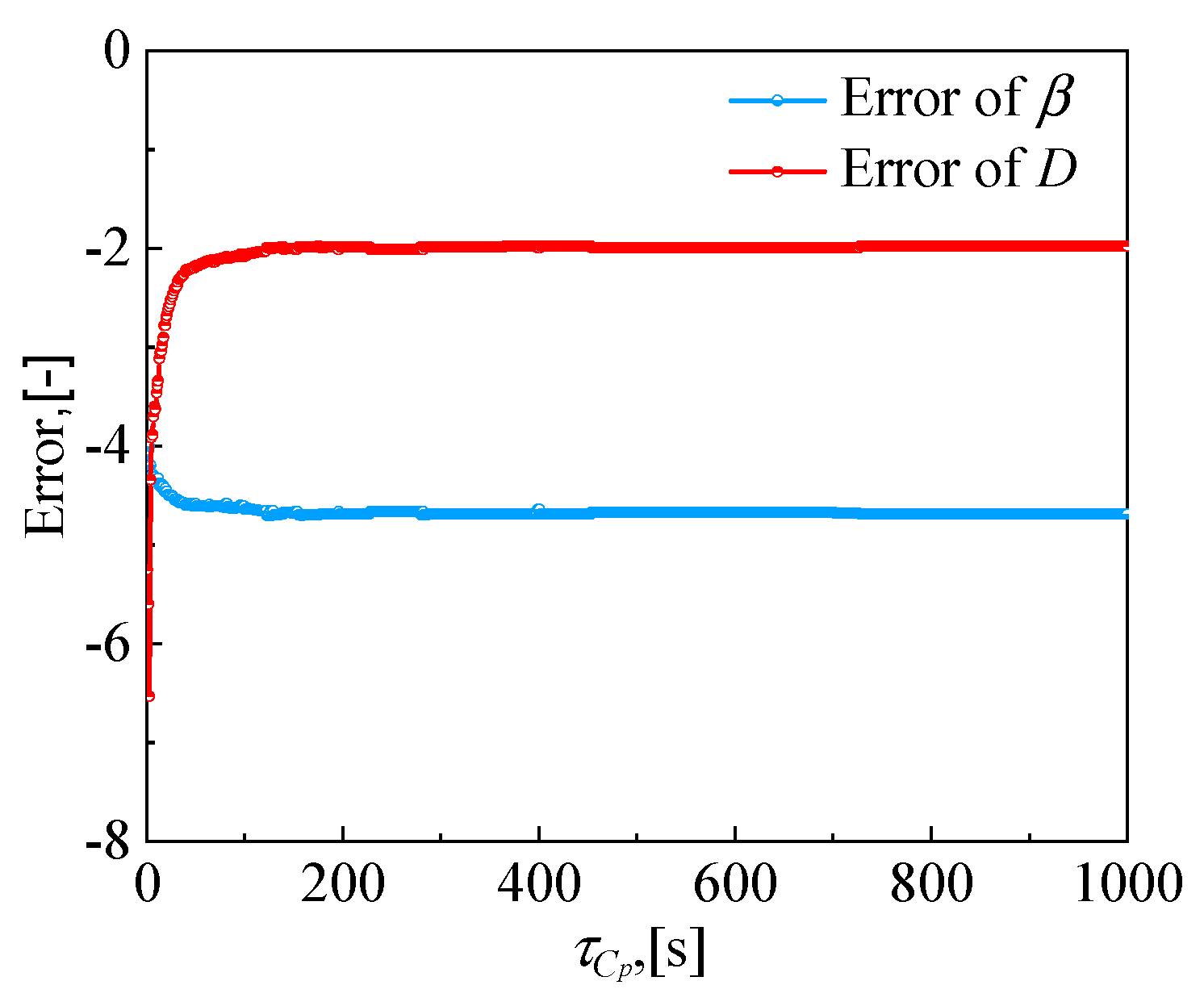
3.2. The Influence of Carbon Potential Build-Up Duration

The sudden change of the carbon potential in the experiment is difficult to achieve, so the influence of carbon potential build-up duration τ_Cp needs to be discussed. Equations (10) and (20) are used to simulate the ECR data and the input parameters are given in

Table 2. Parameters of conductivity relaxation with different τ_Cp.

Bi	β (cm/s)	D (cm2/s)	La (cm)	Lb (cm)	Lb/La	τCp (s)
1	1 × 10−4	1 × 10−6	1 × 10−2	5 × 10−1	50	0
						10
						50
						100
						500
						1000

. All parameters are constant except the duration of carbon potential buildup τ_Cp, which is changed from 0 to 1000. Figure 7 shows the conductivity relaxation curves of different τ_Cp. From the diagram, the relaxation time increases with the value of τ_Cp increasing because of the C potential taking longer to reach its maximum value that affects the diffusion driver. Therefore, τ_Cp needs to be as small as possible.

Figure 8 shows the impedance spectroscopy of different τ_Cp. As shown in Figure 8a, a clear high-frequency induction loop is generated, which is manifested as the high-frequency band of the impedance spectroscopy extending from the first quadrant to the fourth quadrant, and it can be seen from each diagram that with the prolongation of the flush time τ_Cp, the induction loop becomes more and more obvious; that is, the high frequency band continues to extend in the direction of the increase in the imaginary part. By fitting Equation (23) with the data in the impedance spectroscopy, the errors of β and D are derived as shown in Figure 9.

As shown in Figure 9, when Bi = 1 and L_b/L_a = 50, the error of β decreases with the increase in τ_Cp, when τ_Cp is relatively small. After τ_Cp reaches about 150, the error of β remains basically the same. In contrast, the error of D increases with the increase in τ_Cp, and it remains largely unchanged after τ_Cp arrives at 150. Though the error of β keeps getting smaller, the relative error has little change, and considering the change of the error of D, τ_Cp needs to be as small as possible.

Contour maps of errors with different width-to-thickness ratio (1~50) and carbon potential build-up duration (1~100) are shown in Figure 10.

Figure 10a,b show that when Bi = 0.01 and Bi = 1, the increase of the width-to-thickness ratio and τ_Cp could make the error be a smaller value. As shown in Figure 10c,d, the error of D raises with the larger τ_Cp. Meanwhile, it becomes smaller when the width-to-thickness ratio goes down. The observed phenomena all coincide with the previous discussion. If τ_Cp cannot achieve a small value, appropriate increase in the width-to-thickness ratio (more than 50) is proper with Bi = 1. However, the error in the region where τ_Cp is less than 10 is somewhat confusing in Figure 10c, which may be due to the presence of redundant feature time that affects the fitting of (β, D).

4. Conclusions

By combining with the corresponding relationship between the impedance spectroscopy and the Biot number, the one-dimensional conductivity relaxation impedance spectroscopy model is used to fit the two-dimensional conductivity relaxation impedance spectroscopy. The feasibility of the one-dimensional model in practical experiments is discussed, which has certain guiding significance for experiments. The main conclusions are as follows:

(1)

The width-to-thickness ratio of sample in the experiment should be kept above 50, which can ensure the accuracy of the values of (β, D).

(2)

The duration of carbon potential build-up τ_Cp should be as small as possible to ensure the accuracy of the diffusion coefficient D. If τ_Cp is not small enough, a larger width-to-thickness ratio (more than 50) is proper with Bi = 1.

(3)

The ECR method shows the feasibility of measuring the values of (β, D) and even the value of τ_Cp in practical experiments.

References

1. Thete, M.M. Runner-up Simulation of Gas Carburising: Development of Computer Program with Systematic Analyses of Process Variables Involved. Surf. Eng. 2003, 19, 217–228. [Google Scholar] [CrossRef]
2. Moiseev, B.; Brunzel, Y.M.; Shvartsman, L. Kinetics of carburizing in an endothermal atmosphere. Met. Sci. Heat Treat. 1979, 21, 437–442. [Google Scholar] [CrossRef]
3. Ruck, A.; Monceau, D.; Grabke, H.J. Effects of tramp elements Cu, P, Pb, Sb and Sn on the kinetics of carburization of case hardening steels. Steel Res. 1996, 67, 240–246. [Google Scholar] [CrossRef]
4. Turpin, T.; Dulcy, J.; Gantois, M. Carbon diffusion and phase transformations during gas carburizing of high-alloyed stainless steels: Experimental study and theoretical modeling. Metall. Mater. Trans. A 2005, 36, 2751–2760. [Google Scholar] [CrossRef]
5. Yan, M.; Liu, Z. The Mathematical Model of Surface Carbon Concentration Growth during Gas Carburization. Chin. J. Mater. Res. 1992, 6, 223–226. [Google Scholar]
6. Karabelchtchikova, O.; Sisson, R.D. Carbon Diffusion in Steels: A Numerical Analysis Based on Direct Integration of the Flux. J. Phase Equilibria Diffus. 2006, 27, 598–604. [Google Scholar] [CrossRef]
7. Allen, S.M.; Balluffi, R.W.; Carter, W.C. Kinetics of Materials; John Wiley & Sons: New York, NY, USA, 2005; pp. 99–114. ISBN 978-0-471-24689-3. [Google Scholar]
8. Yan, M.; Liu, Z. Study on the distribution function of carbon concentration in the carburized layer of 20 steel during gas carburization in a multi-purpose furnace. Mater. Sci. Technol. 1997, 5, 3. [Google Scholar]
9. Peng, Y.; Zhe, L.; Yong, J.; Bo, W.; Gong, J.; Somers, M. Experimental and numerical analysis of residual stress in carbon-stabilized expanded austenite. Scr. Mater. 2018, 157, 106–109. [Google Scholar] [CrossRef]
10. Christiansen, T.L.; Somers, M. The Influence of Stress on Interstitial Diffusion—Carbon Diffusion Data in Austenite Revisited. Defect Diffus. Forum 2010, 297, 1408–1413. [Google Scholar] [CrossRef]
11. Liu, Z.; Zhang, S.; Wang, S.; Feng, Y.; Peng, Y.; Gong, J.; Somers, M. Redistribution of carbon and residual stress in low-temperature gaseous carburized austenitic stainless steel during thermal and mechanical loading. Surf. Coat. Technol. 2021, 426, 127809. [Google Scholar] [CrossRef]
12. Niessen, F.; Villa, M.; Danoix, F.; Hald, J.; Somers, M. In-situ analysis of redistribution of carbon and nitrogen during tempering of low interstitial martensitic stainless steel. Scr. Mater. 2018, 154, 216–219. [Google Scholar] [CrossRef]
13. Yan, M. Mathematical Modeling and Computer Simulation of Gas Carburization and Rare Earth Carburization Processes. Ph.D. Thesis, Harbin Institute of Technology, Harbin, China, 1993. [Google Scholar]
14. Hummelshoj, T.S.; Christiansen, T.; Somers, M. Determination of Concentration Dependent Diffusion Coefficients of Carbon in Expanded Austenite. Defect Diffus. Forum 2008, 273, 306–311. [Google Scholar] [CrossRef]
15. Gao, W.; Long, J.M.; Kong, L.; Hodgson, P.D. Influence of the Geometry of an Immersed Steel Workpiece on Mass Transfer Coefficient in a Chemical Heat Treatment Fluidised Bed. ISIJ Int. 2004, 44, 869–877. [Google Scholar] [CrossRef]
16. Bengtson, A. Quantitative depth profile analysis by glow discharge. Spectrochim. Acta Part B At. Spectrosc. 1994, 49, 411–429. [Google Scholar] [CrossRef]
17. Angeli, J.; Bengtson, A.; Bogaerts, A.; Hoffmann, V.; Hodoroaba, V.D.; Steers, E. Glow discharge optical emission spectrometry: Moving towards reliable thin film analysis–A short review. J. Anal. At. Spectrom. 2003, 18, 670–679. [Google Scholar] [CrossRef]
18. Shimizu, K.; Habazaki, H.; Skeldon, P.; Thompson, G.E.; Wood, G.C. Influence of argon pressure on the depth resolution during GDOES depth profiling analysis of thin films. Surf. Interface Anal. 2015, 29, 155–159. [Google Scholar] [CrossRef]
19. Bellini, S.; Cilia, M.; Piccolo, E.L. Innovative sample preparation for GDOES analysis of decarburized layers in cylindrical metal specimens. Surf. Interface Anal. 2001, 31, 1100–1103. [Google Scholar] [CrossRef]
20. Kilner, J.A. Measuring oxygen diffusion and oxygen surface exchange by conductivity relaxation. Solid State Ion. 2000, 136, 997–1001. [Google Scholar] [CrossRef]
21. Yasuda, I.; Hishinuma, M. Electrical Conductivity and Chemical Diffusion Coefficient of Strontium-Doped Lanthanum Manganites. J. Solid State Chem. 1996, 123, 382–390. [Google Scholar] [CrossRef]
22. Yeh, T.C.; Routbort, J.L.; Mason, T.O. Oxygen transport and surface exchange properties of Sr0.5Sm0.5CoO3-δ. Solid State Ion. 2013, 232, 138–143. [Google Scholar] [CrossRef]
23. Chen, D.; Shao, Z. Surface Exchange and Bulk Diffusion Properties of Ba0.5Sr0.5Co0.8Fe0.2O3-δ Mixed Conductor. Int. J. Hydrogen Energy 2011, 36, 6948–6956. [Google Scholar] [CrossRef]
24. Grimaud, A.; Bassat, J.M.; Mauvy, F.; Pollet, M.; Wattiaux, A.; Marrony, M.; Grenier, J.C. Oxygen reduction reaction of PrBaCo2-xFexO5+δ compounds as H+-SOFC cathodes: Correlations with physical properties. J. Mater. Chem. A 2014, 2, 3594–3604. [Google Scholar] [CrossRef]
25. Lei, Z.; Liu, Y.; Zhang, Y.; Xiao, G.; Chen, F.; Xia, C. Enhancement in surface exchange coefficient and electrochemical performance of Sr2Fe1.5Mo0.5O6 electrodes by Ce0.8Sm0.2O1.9 nanoparticles. Electrochem. Commun. 2011, 13, 711–713. [Google Scholar] [CrossRef]
26. Egger, A.; Bucher, E.; Sitte, W. Oxygen Exchange Kinetics of the IT-SOFC Cathode Material Nd2NiO4+δ and Comparison with La0.6Sr0.4CoO3-δ. J. Electrochem. Soc. 2015, 158, 573–579. [Google Scholar] [CrossRef]
27. Gopal, C.B.; Haile, S.M. An electrical conductivity relaxation study of oxygen transport in samarium doped ceria. J. Mater. Chem. A 2014, 2, 2405–2417. [Google Scholar] [CrossRef] [Green Version]
28. Wang, Y.; Yan, F.; Zhang, Y.; Xu, Y.; Yan, M. Impedance spectrum model for in situ characterization of the kinetic equation parameters of vacuum thermal expansion. J. Mater. Heat Treat. 2020, 41, 129–134. [Google Scholar] [CrossRef]
29. Magar, H.S.; Hassan, R.Y.; Mulchandani, A. Electrochemical impedance spectroscopy (EIS): Principles, construction, and biosensing applications. Sensors 2021, 21, 6578. [Google Scholar] [CrossRef]
30. Crank, B.J. The Mathematics of Diffusion, 2nd ed.; Oxford University Press: New York, NY, USA, 1975; pp. 60–61. ISBN 978-01-9853-411-2. [Google Scholar]
31. Ciucci, F. Electrical conductivity relaxation measurements: Statistical investigations using sensitivity analysis, optimal experimental design and ECRTOOLS. Solid State Ion. 2013, 239, 28–40. [Google Scholar] [CrossRef]
32. Boukamp, B.A.; den Otter, M.W.; Bouwmeester, H.J.M. Transport processes in mixed conducting oxides: Combining time domain experiments and frequency domain analysis. J. Solid State Electrochem. 2004, 8, 592–598. [Google Scholar] [CrossRef]
33. Otter, M.D.; Bouwmeester, H.; Boukamp, B.A.; Verweij, H. Reactor Flush Time Correction in Relaxation Experiments. J. Electrochem. Soc. 2001, 148, J1. [Google Scholar] [CrossRef]
Figure 1. Schematic diagram of gas carburization process and the experimental setup. (a) flow diagram of gas carburizing process, (b) schematic diagram of the experimental setup, (c) schematic diagram of the experimental principle.
Coatings 12 01886 g001
Figure 2. Conductivity relaxation curves of different Bi. (a) Bi = 0.01, (b) Bi = 1, (c) Bi = 100.
Coatings 12 01886 g002
Figure 3. Impedance spectroscopy of different width-to-thickness ratios (Bi = 0.01). (a) Nyquist figure, (b) variation curve of real part and imaginary part with frequency.
Coatings 12 01886 g003
Figure 4. Impedance spectroscopy of different width-to-thickness ratios (Bi = 1). (a) Nyquist figure, (b) variation curve of real part and imaginary part with frequency.
Coatings 12 01886 g004
Figure 5. Impedance spectroscopy of different width-to-thickness ratios (Bi = 100). (a) Nyquist figure, (b) variation curve of real part and imaginary part with frequency.
Coatings 12 01886 g005
Figure 6. Errors of β and D with different Bi.
Coatings 12 01886 g006
Figure 7. Conductivity relaxation curves of different τCp.
Coatings 12 01886 g007
Figure 8. Impedance spectroscopy of different τCp (Bi = 1). (a) Nyquist figure, (b) variation curve of real part and imaginary part with frequency.
Coatings 12 01886 g008
Figure 9. Errors of β and D with different τCp (Bi = 1).
Coatings 12 01886 g009
Figure 10. Contour maps of errors with different width-to-thickness ratios and carbon potential build-up durations. (a) error of β (Bi = 0.01), (b) error of β (Bi = 1), (c) error of D (Bi = 1), (d) error of D (Bi = 100).
Coatings 12 01886 g010