Article

Element Differential Method for Non-Fourier Heat Conduction in the Convective-Radiative Fin with Mixed Boundary Conditions

1
School of Automobile, Chang’an University, Xi’an 710064, China
2
School of Power and Energy, Northwestern Polytechnical University, Xi’an 710072, China
*
Author to whom correspondence should be addressed.
Coatings 2022, 12(12), 1862; https://doi.org/10.3390/coatings12121862
Submission received: 30 October 2022 / Revised: 25 November 2022 / Accepted: 29 November 2022 / Published: 30 November 2022
(This article belongs to the Special Issue Micro/Nanomaterials for Heat Transfer, Energy Storage and Conversion)

Abstract

:
Fin is an efficient and straightforward way to enhance heat transfer rate. When the heat source varies dramatically in a very short time, non-Fourier heat conduction should be considered. In the paper, taking advantage of numerical stability and no integral and easy-to-implement features of an element differential method, a numerical model is developed to evaluate the fin efficiency of the convective-radiative fin within non-Fourier heat conduction. In this fin, heat is generated by an internal heat source and dissipated by convection and radiation. Both periodic and adiabatic boundary conditions are considered. The accuracy and efficiency of the element differential method is validated by several numerical examples with analytical solutions. The results indicate that the element differential method has high precision and flexibility to solve non-Fourier heat conduction in convective-radiative fin. Besides, the effects of Vernotte number, dimensionless periodicity, thermal conductivity coefficient, and emissivity coefficient on dimensionless fin tip temperature, instantaneous fin efficiency, and average fin efficiency are comprehensively analyzed.

1. Introduction

Many machines widely use the fin as an efficient and straightforward heat exchanger, such as jet engines, microelectronic components, oil pipelines, etc. Fin exchanges heat with the environment through radiation and convection. Generally, when the working conditions are stable and the time is long enough, the Fourier law can describe conductive heat transfer in the steady-state fin. However, when the heat source changes dramatically or the time of the transient problem is too short, the Fourier model is not suitable. For example, for heat dissipation in microelectronic elements, heat flux density is close to that produced by nuclear fusion, and Fourier’s law is unsuitable in this situation [1]. Cattaneo [2] and Vernotte [3] introduced a hyperbolic heat conduction model with a finite propagation speed. This is the well-known non-Fourier heat conduction model, which can be expressed as follows,
τ q t + q = k T
where τ = α / v 2 represents relaxation time, α is the thermal diffusivity, and v is the velocity of the heatwave. When the velocity of the heatwave is finite, the relaxation time τ is not equal to zero [4]. As early as the 1980s, Lin [5] used the Laplace transform technique to study the periodic heat fin and pointed out that the Fourier model brings a significant error when the thermal relaxation time is greater than the period of oscillation. Das et al. [6] used the genetic algorithm to retrieve parameters in non-Fourier conduction and radiation heat transfer and convective-radiative fin with temperature-dependent thermal conductivity. Zahra et al. [7] used the spectral-finite volume method to analyze non-Fourier heat transfer in convective fin. In this paper, sinusoidal, triangular, and square periodic base temperatures were both considered.
In recent years, with the increasing application of fin in various fields, the working condition of the fin is becoming more and more complex, such as porous fin [8], irregular fins [9,10], and transient wet fin [11]. Das and Kundu [12] adopted an inverse approach to solving conductive heat transfer of the wet fin. Mehraban et al. [13] developed the θ method to predict the thermal performance of the convective-radiative porous fin with periodic thermal conditions. Gireesha et al. [14] used the finite element method (FEM) to study the temperature performance of porous fin within the fully wet condition. Prakash et al. [15] investigated the effect of thermal radiation on nanofluid flow [16,17].
Unlike the above numerical methods, the element differential method (EDM) [18] is a strong-form technique to solve ordinary or partial differential equations. The most important feature of the EDM is that the derived spatial derivatives can be directly substituted into the governing equation and boundary conditions to form the final system of algebraic equations [19]. Therefore, the EDM does not require any mathematical principles or integrations and is very easy to code. Cui et al. [20] proved that the EDM was a high-efficiency method to solve nonlinear heat transfer with the internal heat source by solving the two-dimensional and three-dimensional fins.
In this paper, the EDM is first developed to solve nonlinear heat transfer of convective-radiative fin with mixed boundary conditions in Fourier and non-Fourier models. At the same time, the effects of radiation and a nonlinear internal heat source are considered. In practice, these fin parameters, such as the surface emissivity, thermal conductivity, heat transfer coefficient, and internal heat source, are the functions of temperature instead of constants. The effects of the parameters mentioned above on the instantaneous fin tip temperature and fin efficiency are comprehensively analyzed.
This paper is organized as follows. The physical and mathematical models are presented in Section 2. The principle of EDM and the discretized scheme of the nonlinear heat transfer equation of convective-radiative fin are described in Section 3. The validation of this method is verified from the analytical solution in Section 4. Then, the results and discussions are stated in Section 5. Finally, conclusions are summarized in Section 6.

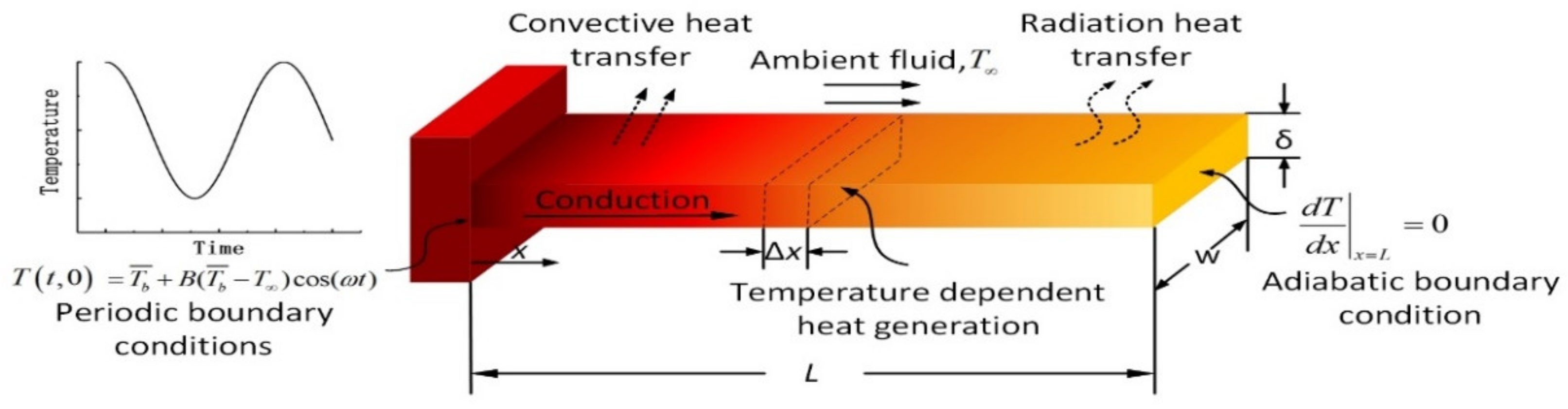
2. Physical and Mathematical Models

As shown in Figure 1, a longitudinal rectangular fin with the cross-sectional area A c , thickness δ, length L, and perimeter P is considered. The thickness is minimal compared with the length of the fin. There is convection and radiation in the heat exchange between the fin surface and ambient fluid, and the internal heat source of the fin is also considered. The following assumptions are made to obtain the governing equation,
  • The ambient temperature T remains unchanged and is not affected by fin heat dissipation.
  • The non-Fourier heat conduction is considered in one dimension.
  • The radiation between the fin and fin base is ignored.
  • The fin base temperature is maintained at periodic oscillation, and the fin tip is adiabatic.
  • Similar as Ref. [21], thermal conductivity, surface emissivity, heat transfer coefficient, and internal heat generation rate are both assumed as temperature dependent and expressed as follows,
k T = k 1 + μ T T T b , m T
ε ( T ) = ε 1 + ξ T T T b , m T
h ( T ) = h T T T b , m T b
q * ( T ) = c 1 + c 2 T T T b , m T + c 3 T T T b , m T 2 + c 4 T T T b , m T 3
where k , ε are thermal conductivity and surface emissivity at ambient temperature T , μ , and ξ are coefficients of thermal conductivity and surface emissivity, T b , m is the mean base temperature, h is heat transfer coefficient at fin base, b is the power index of the convective heat transfer coefficient, which depends on the mechanism of convective heat transfer [22]. For example, b = 2 is nucleate boiling heat transfer. c 1 , c 2 , c 3 , and c 4 are the coefficients of internal heat generation rate.
Based on those assumptions, the transient non-Fourier fin heat transfer equation is expressed as [23],
ρ c p T t + h ( T ) p τ A c T t + ε ( T ) σ p τ A c T 4 t τ q * ( T ) t + ρ c p τ 2 T t 2 = x k T T x h ( T ) p A c ( T T ) ε ( T ) σ p A c ( T 4 T 4 ) + q * ( T )
where c p is the specific heat capacity of fin; ρ is the density; σ is the Stefan–Boltzmann constant; τ is the relaxation time.
The initial conditions are,
T x , 0 = T
The fin base is maintained at a periodic temperature oscillation, and the fin tip is adiabatic. The corresponding boundary conditions are,
T L , t x = 0
T 0 , t = T b , m + B ( T b , m T ) cos ( ω t )
For the convenience of analysis, the following dimensionless variable and similarity criteria are introduced,
Θ = T T T b , m T , Θ 0 = T T b , m T , t * = k t ρ c p L 2 , X = x L , Ω = L 2 ω ρ c p k , N r c = p ε σ L 2 A c k T b , m T 3 , N c = h p L 2 A c k , V e = τ k ρ c p L 2 , C 1 = L 2 c 1 T b , m T k , C 2 = L 2 c 2 T b , m T k , C 3 = L 2 c 3 T b , m T k , C 4 = L 2 c 4 T b , m T k
where the Vernotte number Ve is the order of dimensionless relaxation time.
Using Equation (6), Equation (3) can be rewritten in dimensionless form as,
1 + N c 2 V e 2 Θ b + 4 ( 1 + ξ Θ ) N r c V e 2 Θ 3 + 3 Θ 2 Θ 0 + 3 Θ Θ 0 2 + Θ 0 3 V e 2 C 2 + 2 C 3 Θ + 3 C 4 Θ 2 Θ t * + V e 2 2 Θ t * 2 = ( 1 + μ Θ ) 2 Θ X 2 + μ Θ X 2 N c 2 Θ b + 1 ( 1 + ξ Θ ) N r c Θ 4 + 4 Θ 3 Θ 0 + 6 Θ 2 Θ 0 2 + 4 Θ Θ 0 3 + C 1 + C 2 Θ + C 3 Θ 2 + C 4 Θ 3
Using the implicit scheme to discretize the transient term, Equation (7) can be rewritten as,
A Θ k Θ k 1 Δ t * + V e 2 Θ k 2 Θ k 1 + Θ k 2 Δ t * 2 = B 2 Θ k X 2 + μ Θ k X 2 + F
where,
A = 1 + N c 2 V e 2 Θ o l d k b + 4 ( 1 + ξ Θ o l d k ) N r c V e 2 Θ o l d k 3 + 3 Θ o l d k 2 Θ 0 + 3 Θ o l d k Θ 0 2 + Θ 0 3 V e 2 C 2 + 2 C 3 Θ o l d k + 3 C 4 Θ o l d k 2
B = 1 + μ Θ o l d k
F = N c 2 Θ o l d k b + 1 ( 1 + ξ Θ o l d k ) N r c Θ o l d k 4 + 4 Θ o l d k 3 Θ 0 + 6 Θ o l d k 2 Θ 0 2 + 4 Θ o l d k Θ 0 3 + C 1 + C 2 Θ o l d k + C 3 Θ o l d k 2 + C 4 Θ o l d k 3
where, the subscript “ k = 1 , 2 , , N t ” represents the result of the k-time layer, Nt is the number of discretized time steps, and the subscript “old” means the last iterative value.
Similarly, the dimensionless forms of initial and boundary conditions are,
Θ ( X , 0 ) = 0
Θ ( 1 , t * ) X = 0
Θ ( 0 , t * ) = 1 + B cos ( Ω t * )
The instantaneous fin efficiency and the average fin efficiency are,
η = 1 N c 2 Θ b + 1 + ( 1 + ξ ) N r c Θ 4 d Θ d X X = 0
η ave = 1 p e d t * d t * + p e η d t *
where p e = 2 π / Ω is the heat source vibration period.

3. Principle of Element Differential Method

Using iso-parametric elements, we can express the shape function as the Lagrange interpolation formulation,
L i n ( χ ) = j = 1 , j i n χ χ j χ i χ j
where n is the number of interpolation points in each element and χ is the iso-parametric coordinate.
Variables can be approximated by the node values of the iso-parametric element. Thus, the dimensionless temperature can be expressed as,
Θ = j = 1 N e L ( χ j ) Θ j
where, Ne is the number of nodes in the isoparametric element, and Θ j is dimensionless temperature at the node. Based on Equations (12) and (13), the first and second-order derivatives can be expressed as,
Θ X = j = 1 N e L X Θ j
2 Θ X 2 = j = 1 N e 2 L X 2 Θ j
As shown in Figure 2, the computational domain is discretized by isoparametric elements. The nodes are divided into internal, interface, and boundary nodes.
For internal nodes, substituting Equations (13) and (14), Equation (8) can be discretized as,
A Δ t * + V e 2 Δ t * 2 B 2 L X 2 Δ t * 2 μ L X 2 Θ o l d Θ k = ( A Δ t * + 2 V e 2 ) Θ k 1 V e 2 Θ k 2 + Δ t * 2 F
For interface nodes, the sum of heat flux is zero.
f = 1 N f k Θ X n f = 0
where, N f is the number of shared surfaces, superscript f indicates the shared plane, and n f is the normal surface vector.
After substituting Equation (13a), Equation (16) can be rewritten as,
f = 1 N f j = 1 N e k L ( χ j ) X Θ j n f = 0
Using the EDM, the Neumann boundary condition is also be discretized as,
f = 1 N f j = 1 N e k L χ j X Θ j n f = Q i n
where Q i n is input heat flux at the boundary. If the boundary is adiabatic, Q i n = 0 .
Assembling Equations (15), (17) and (18), the system of discrete equations can be written as,
A Θ = d
where A is the coefficient matrix assembled by the internal, interface, and boundary nodes; d is the known vector determined by the source term.
The implementation of EDM for solving non-Fourier heat conduction in convective-radiative fin can be executed by the following steps:
(1)
Discretize the computational domain by isoparametric elements, and determine the number of nodes in each isoparametric element Ne.
(2)
Initialize dimensionless temperature according to the initial condition.
(3)
Loop at each time step, k = 1 , 2 , , N t .
(4)
For each time step, assemble the coefficient matrix A, impose the boundary condition, and assemble the vector d.
(5)
Directly solve the matrix equation (Equation (19)) to obtain the new dimensionless temperature.
(6)
If the convergence criterion ( Θ k Θ o l d k / Θ o l d k < 10 6 ) is satisfied, terminate the iterative, and go to step (7). Otherwise, go back to step (4).
(7)
If the number of time steps is not reached, go to step (3). Otherwise, calculate fin efficiency η .

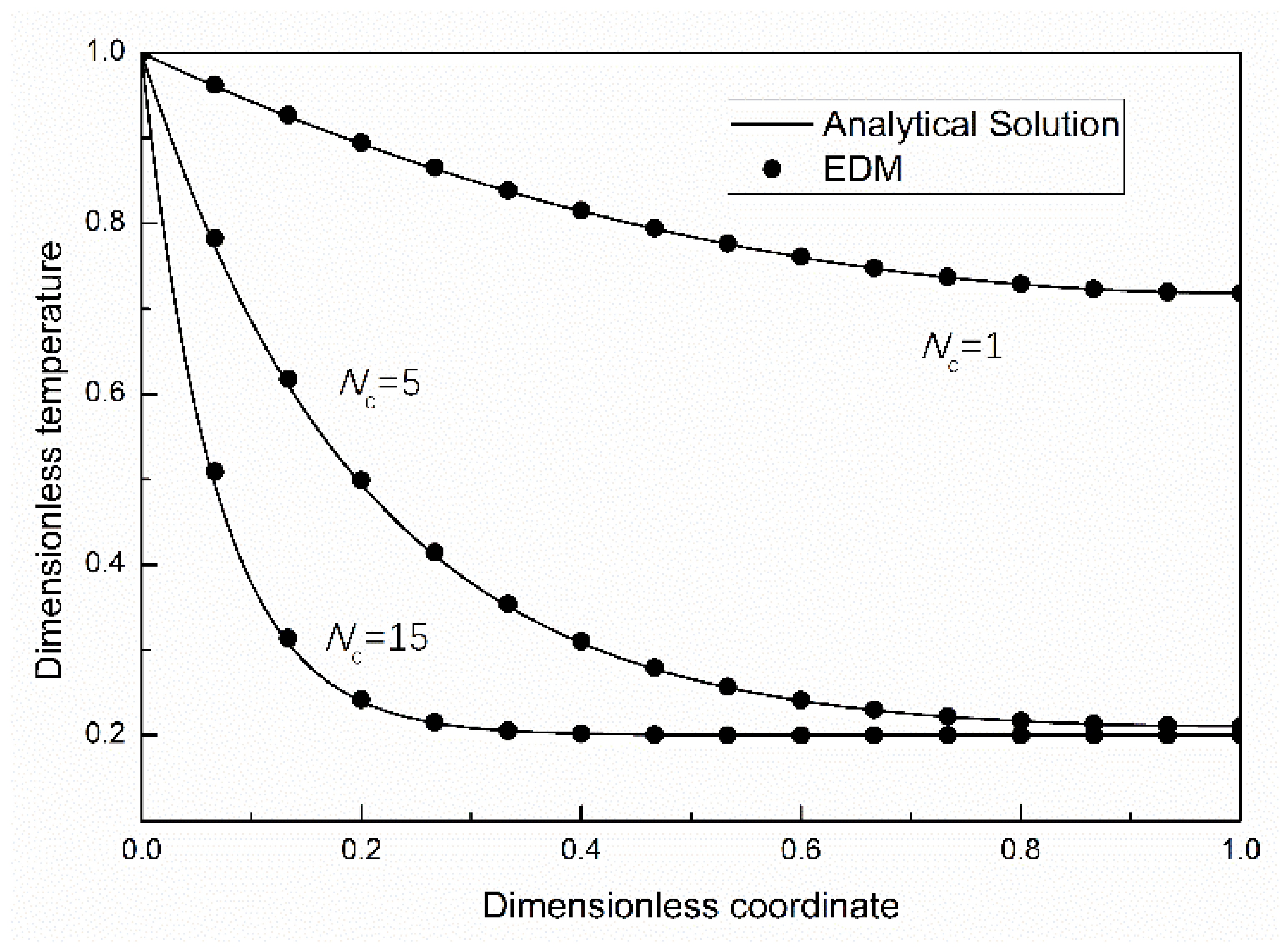
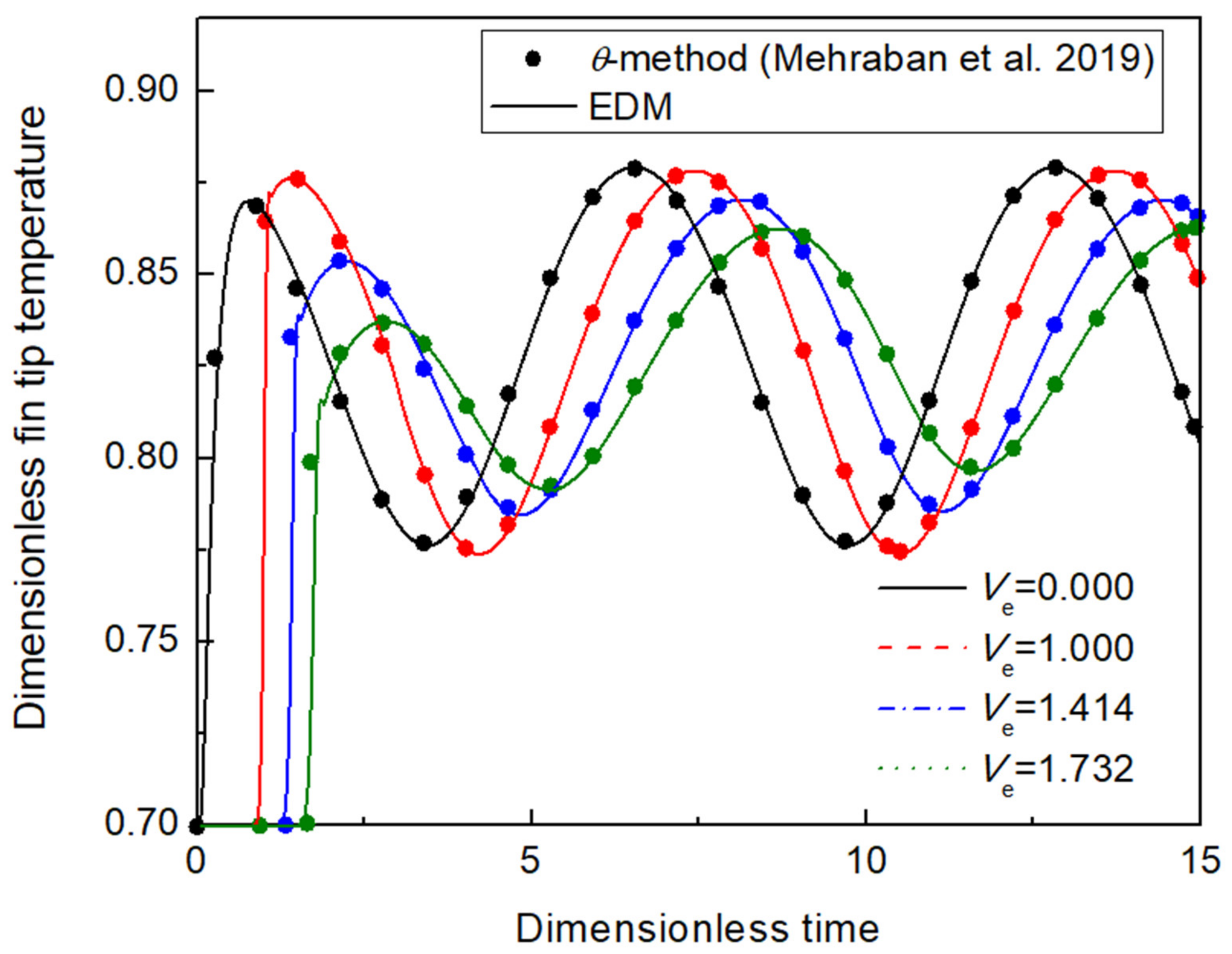
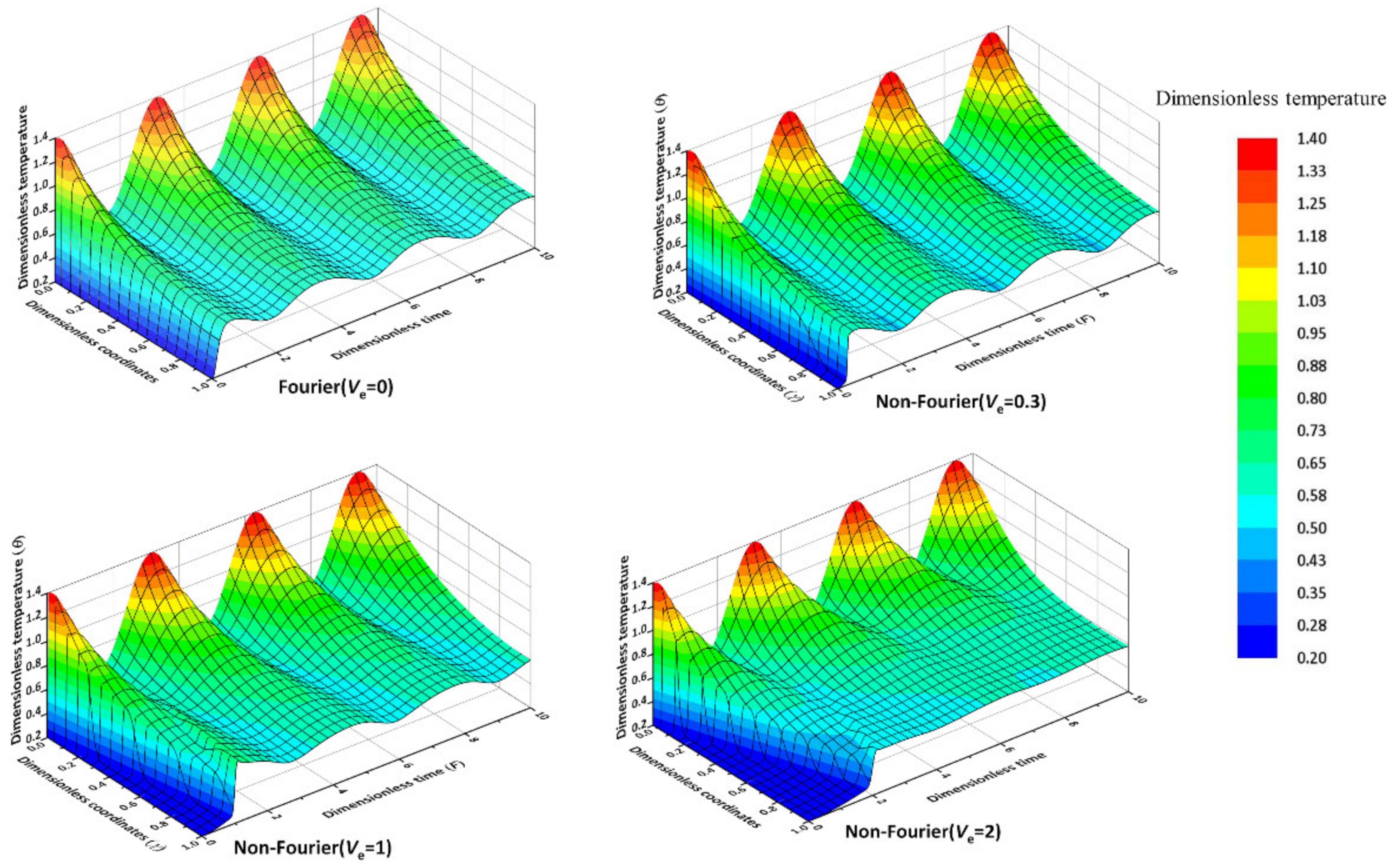
4. Verification of Element Differential Method Solution

To validate the EDM solution, a test case of steady-state Fourier heat transfer was adopted. In this case, the radiative-conductive parameter and an internal heat source are assumed to be zero. Accordingly, the governing equation is simplified as,
2 Θ X 2 = N c 2 Θ
The analytical solution of Equation (20) is,
Θ X = cos h ( N c X N c ) cos h ( N c )
Figure 3 shows the temperature distribution for three convective parameters N c = 1 ,   5 ,   15 . For comparisons, the EDM results and analytical solutions are simultaneously plotted in Figure 3. Compared with analytical solutions, the maximum relative error of the EDM results is 0.17%.
Secondly, to further evaluate the accuracy of the EDM, more comparisons are made. The dimensionless fin tip temperature by the EDM is shown in Figure 4. Figure 4 indicates that the agreement between θ method [13] and EDM results is excellent, and the maximum relative difference is less than 1.36%. Therefore, it can be demonstrated that the EDM can provide an adequately accurate solution for non-Fourier heat conduction in the convective-radiative fin.

5. Results and Discussions

To predict the thermal process of non-Fourier heat conduction in convective-radiative fin, the effects of Vernotte number Ve, dimensionless periodicity Ω, coefficient of thermal conductivity μ, and coefficient of emissivity ξ on temperature and fin efficiency are comprehensively analyzed. In this section, except for special note, these parameters are fixed as: C 1 = C 2 = C 3 = C 4 = 2 , b = 1 , μ = 0.1 , ξ = 0.1 , V e = 1 , N c = 2 , N r c = 2 , Θ 0 = 0.2 , Ω = 2 , B = 0.5 .

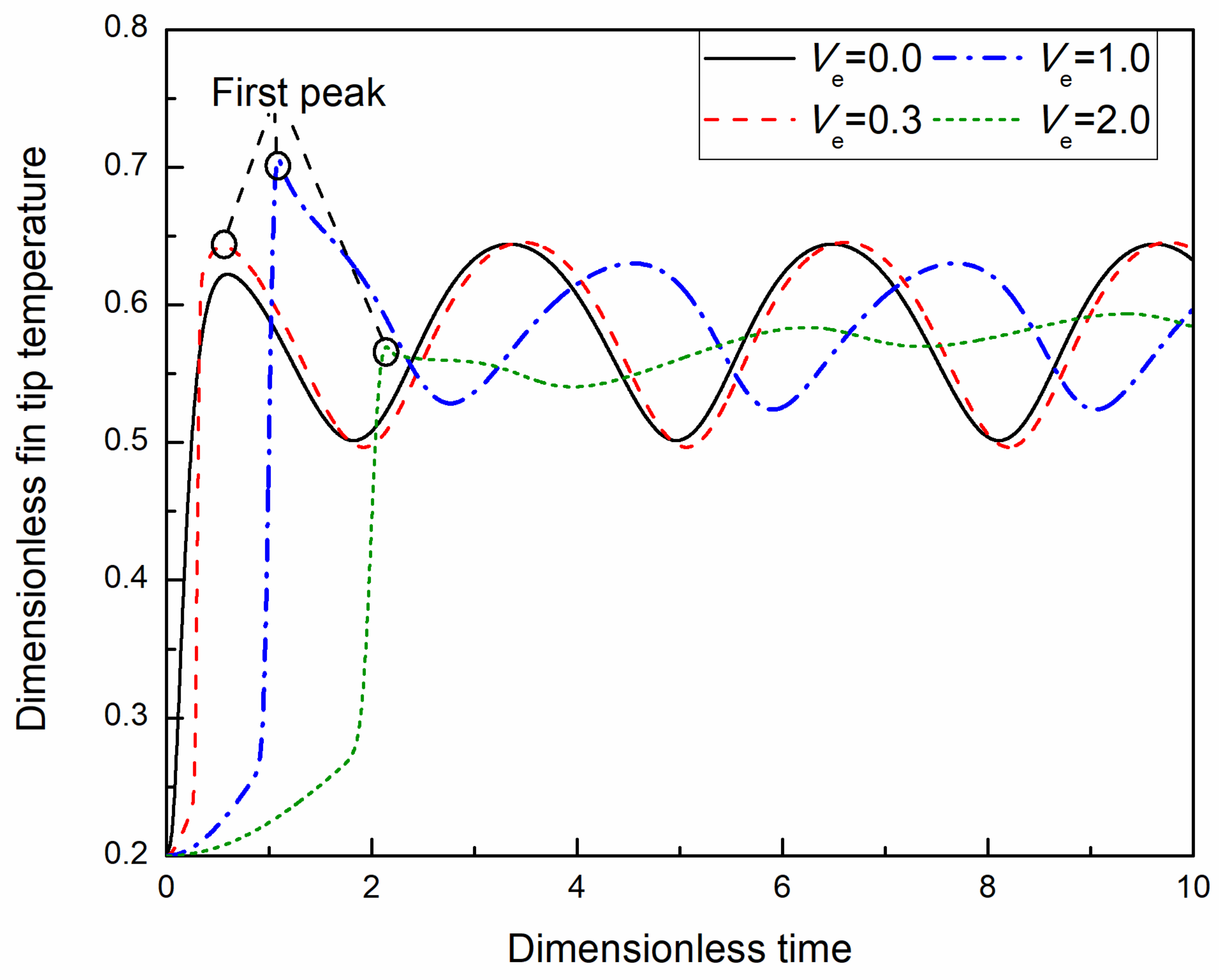
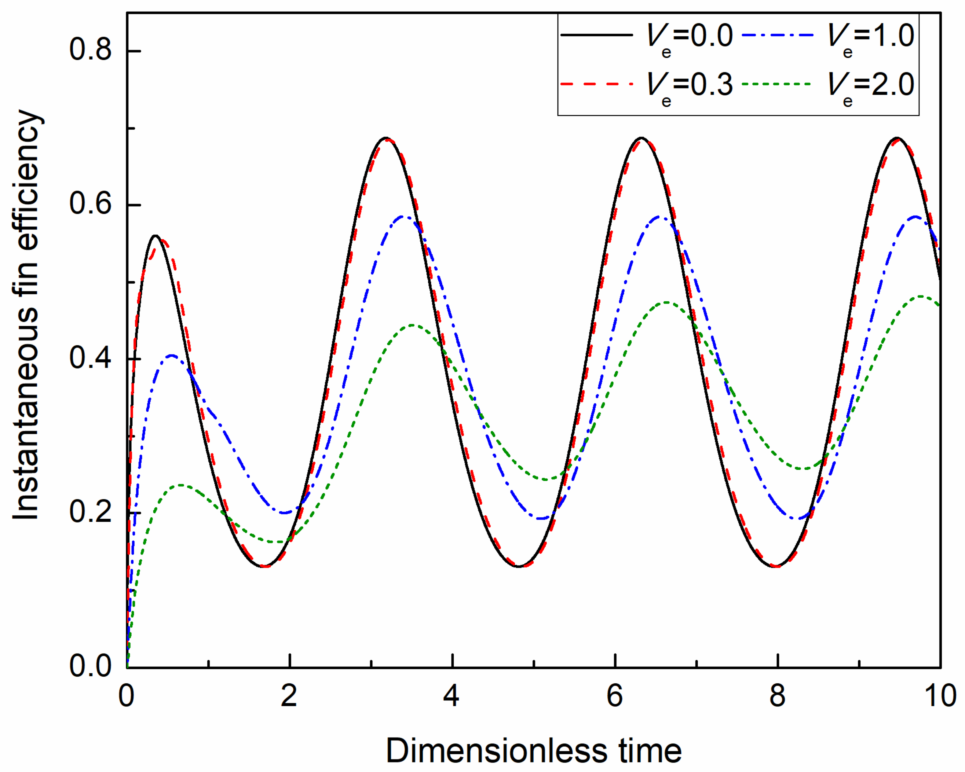
5.1. The Effect of Vernotte Number

The Vernotte number Ve is the order of dimensionless relaxation time. In the case of Ve = 0, the nonlinear heat transfer in the convective-radiative fin is Fourier heat conduction. Figure 5 depicts the variation of dimensionless temperature with position and time in convective-radiative fin for different Vernotte numbers Ve = 0, 0.3, 1.0, and 2.0. At the initial stage, the dimensionless fin temperature excepted at the fin base is constant as Θ 0 = 0.2 . When F > 0 , the periodic fluctuation in temperature is imposed at the base. When the value of F is small, the dimensionless temperature increases sharply, and this phenomenon becomes more apparent in the case of lager Ve. When the value of F is significant, the wave amplitude of temperature becomes smaller as the distance from the fin base increases. This trend becomes more evident as Ve increases. Otherwise, with the passage of dimensionless time, the wave of dimensionless temperature tends to stable, and the stable time is postponed with the increase of Ve.
Figure 6 shows the effect of Ve on fin tip temperature. As time goes on, the fin tip temperature reaches its first peak. Then, the perturbation of the fin tip temperature tends to a quasi-steady state. Otherwise, it also exists the lag phenomena. With the increase of Ve, the lag phenomena tend to be more prominent, and the temperature variation range becomes smaller. The reason is that, with the increase of Ve, the speed of heat propagation becomes slow, and the heat exchange between the fin surface and ambient fluid becomes more efficient.
The effect of Ve on the instantaneous fin efficiency is presented in Figure 7. With the increase of Ve, the dimensionless time at which efficiency reaches the first peak is postponed, and the wave amplitude of efficiency becomes smaller.

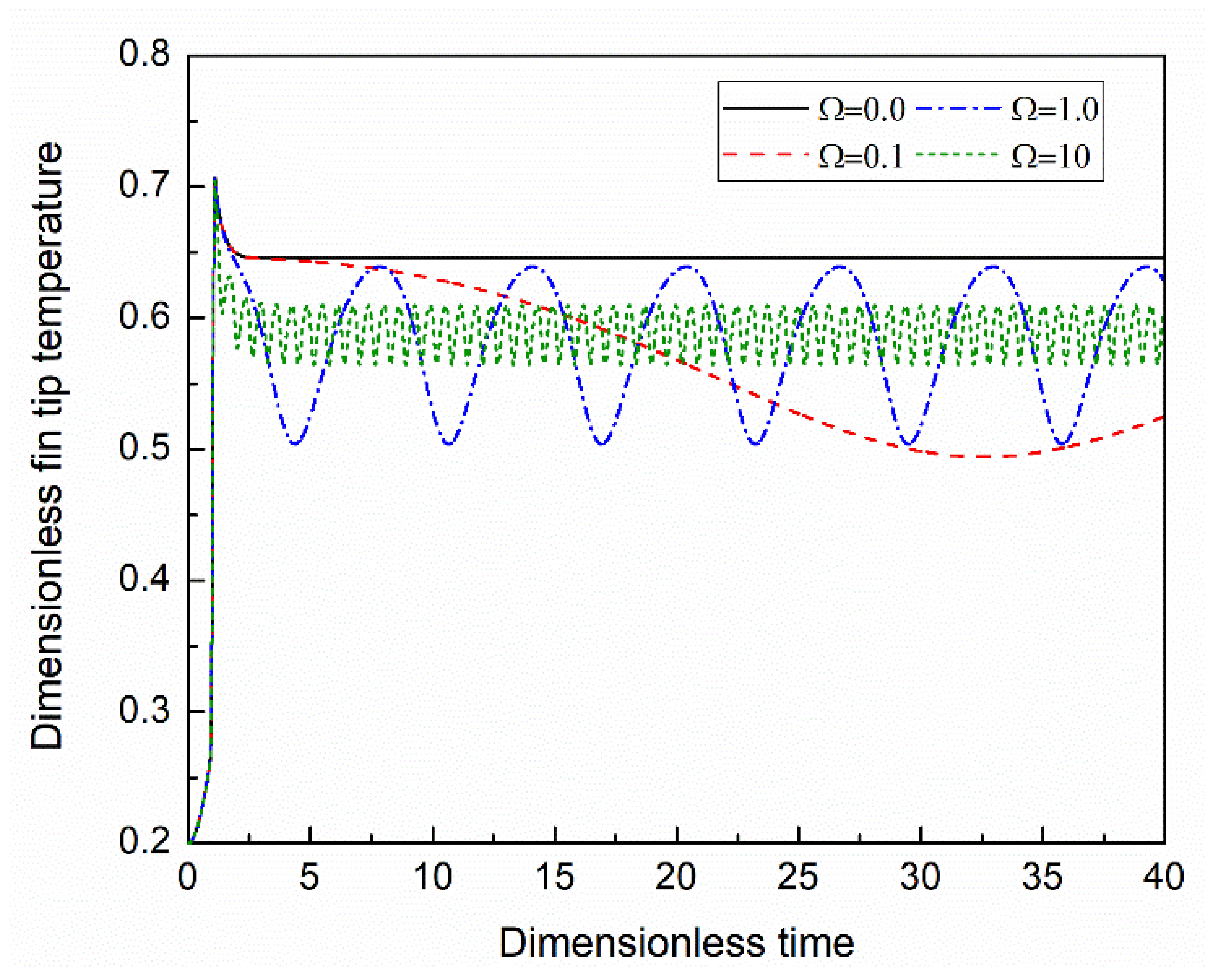
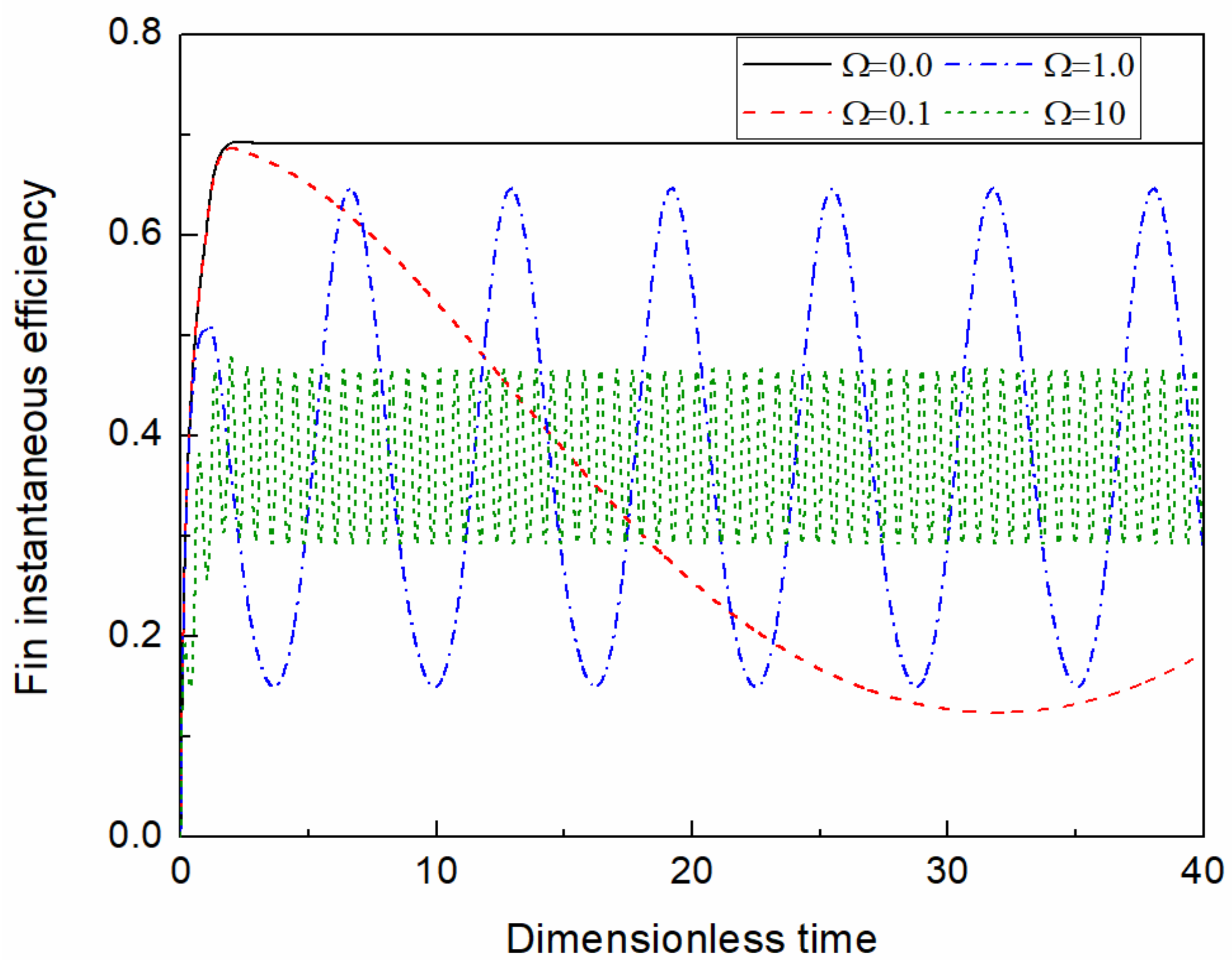
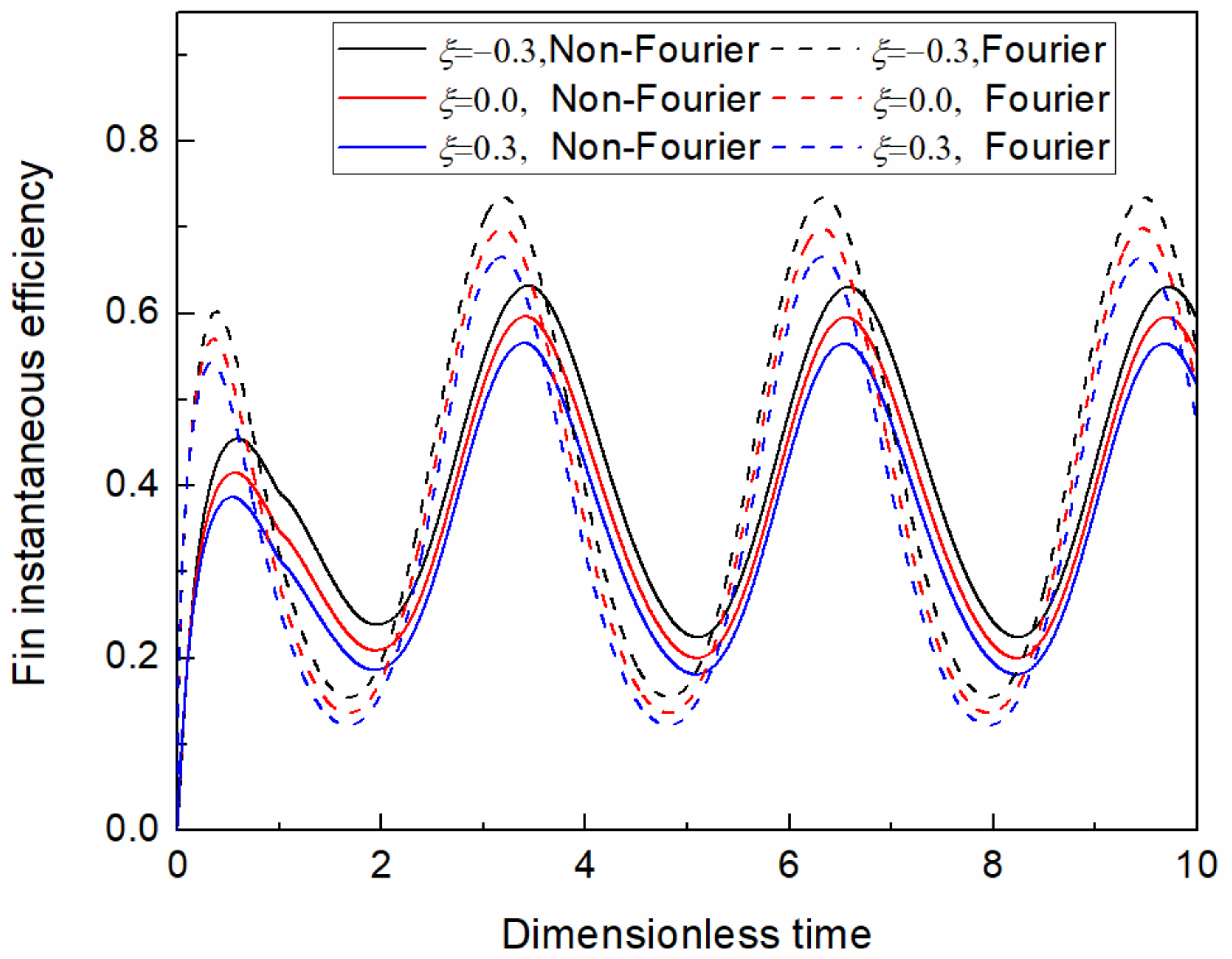
5.2. The Effect of Dimensionless Periodicity

As expressed in Equation (6), dimensionless periodicity Ω = L 2 ω / α is the frequency of periodic boundary conditions. The effect of dimensionless periodicity Ω on dimensionless fin tip temperature is illustrated in Figure 8. Before the heatwave reaches the fin tip (the temperature of the fin tip suddenly rises), the effect of Ω on dimensionless fin tip temperature can be omitted, and the increasing values of dimensionless fin tip temperature for different values of Ω are the same. As time goes on, the dimensionless fin tip temperature decreases rapidly. With the further passage of time, the variation of dimensionless fin tip temperature tends to be stable and is not influenced by the initial condition. The variation range of dimensionless fin tip temperature becomes smaller as Ω increases.
Figure 9 shows the effect of Ω on instantaneous fin efficiency. Before the heatwave reaches the fin tip, the increasing gradients of instantaneous fin efficiency are consistent for different values of Ω. With the passage of time, the value of instantaneous fin efficiency is fixed for the Fourier model ( Ω = 0 ). However, the value of instantaneous fin efficiency tends to fluctuate for the non-Fourier model ( Ω 0 ). When Ω increases, the first peak value of instantaneous fin efficiency decreases, and amplitude becomes smaller and frequency increases.

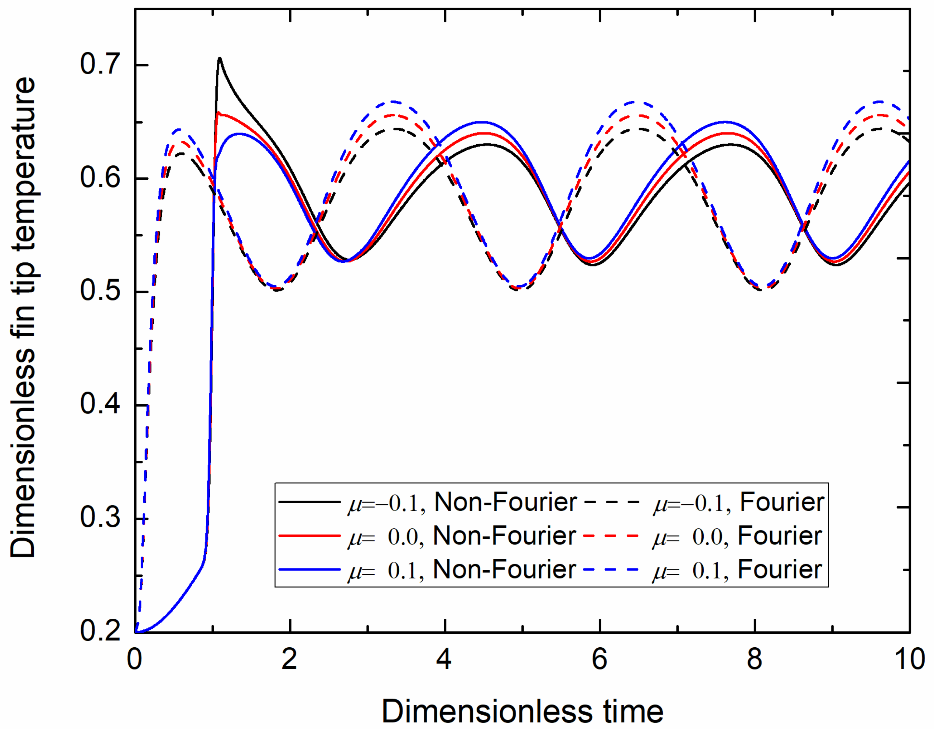
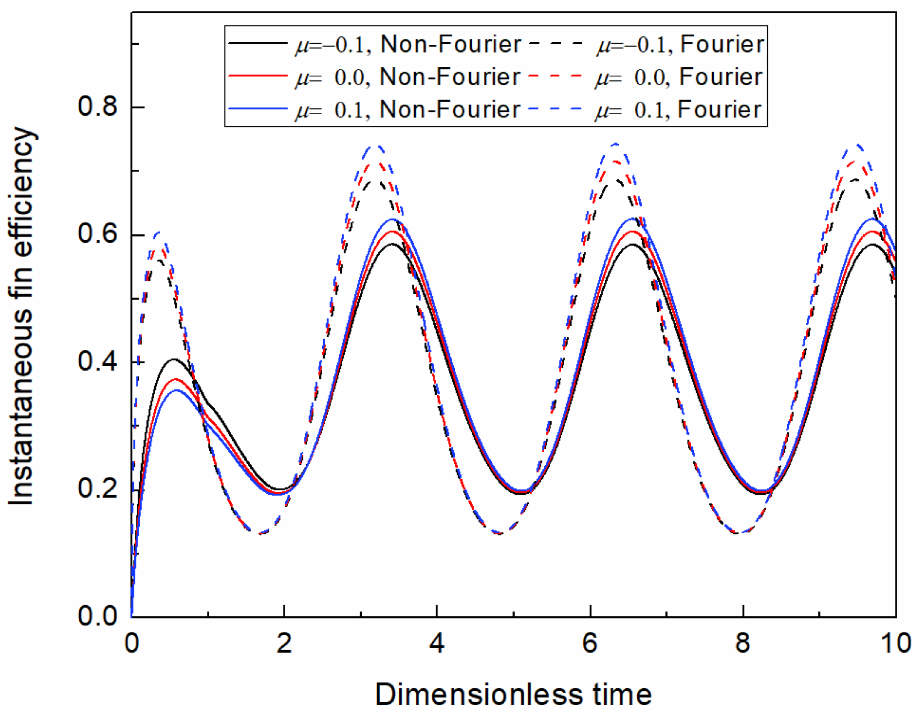
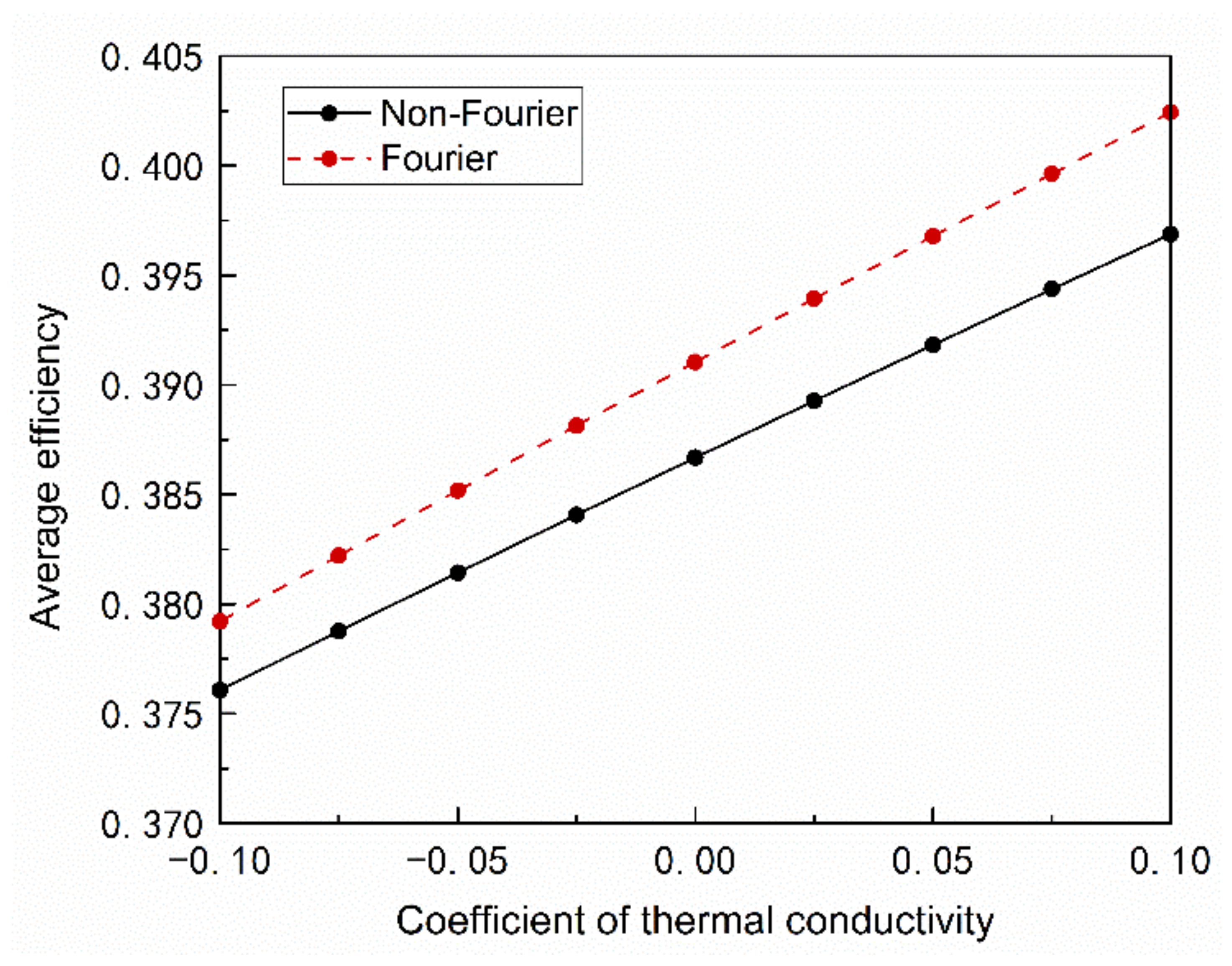
5.3. The Effect of Coefficient of Thermal Conductivity

To understand the influence of the coefficient of thermal conductivity on transient heat transfer in convective-radiative fin, an assessment is made in Figure 10, Figure 11 and Figure 12. Figure 10 exhibits the variation of dimensionless fin tip temperature with three values of coefficient of thermal conductivity (namely μ = 0.1 , 0.0 , 1.0 ). It is seen that the higher value of μ depicts the larger wave amplitude for the Fourier model. When the first heat wave arrives, the higher value of μ obtains the lower dimensionless fin tip temperature for the non-Fourier model. However, when the temperature fluctuation tends to be stable, the higher value of μ can obtain the larger wave amplitude of dimensionless fin tip temperature for the non-Fourier model. A similar change trend of instantaneous fin efficiency is also found in Figure 11.
Figure 12 presents the variation of average fin efficiency with different values of μ. The average fin efficiency increases with the increase of μ. Furthermore, the average fin efficiency of the Fourier model is higher than that of the non-Fourier model.

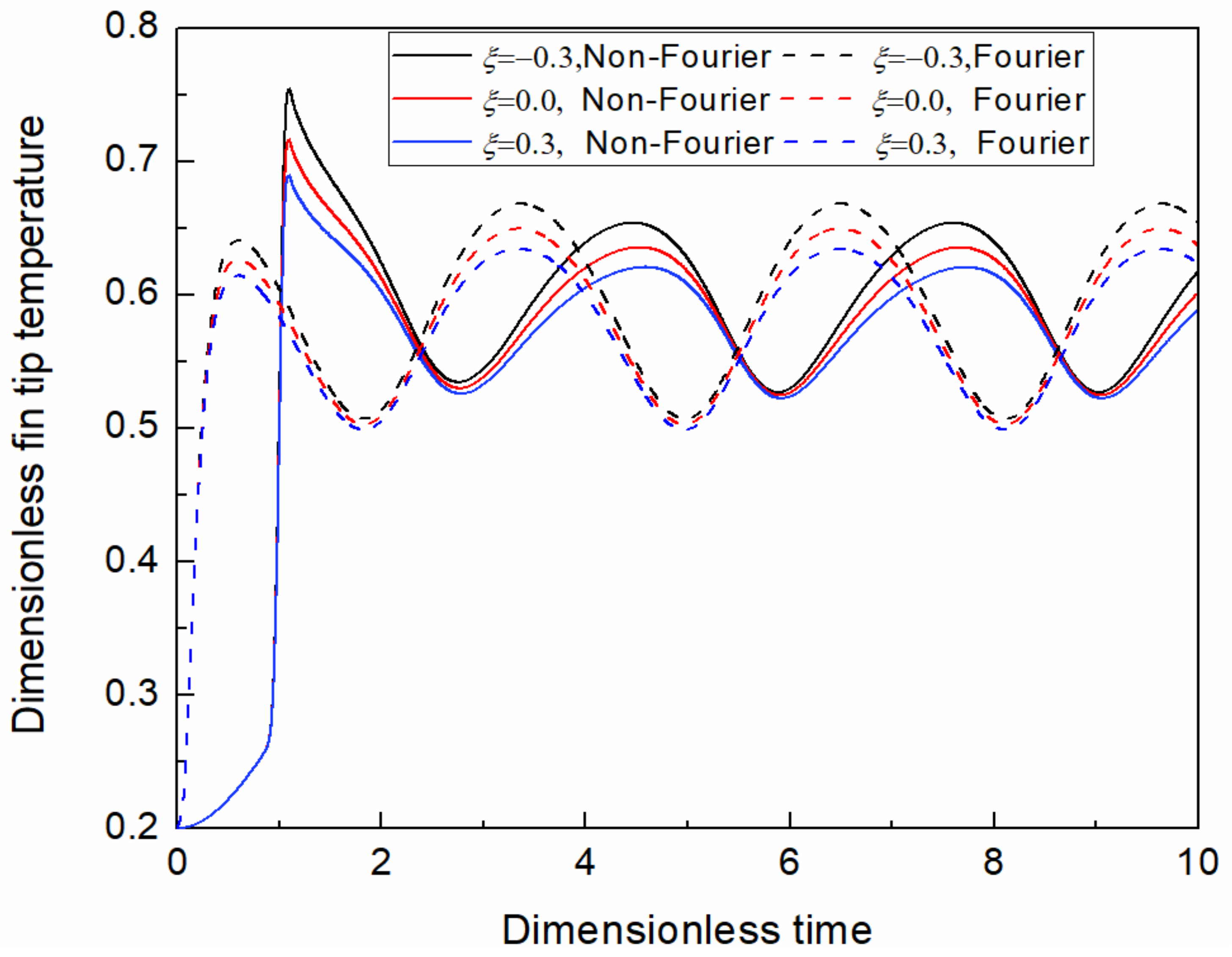
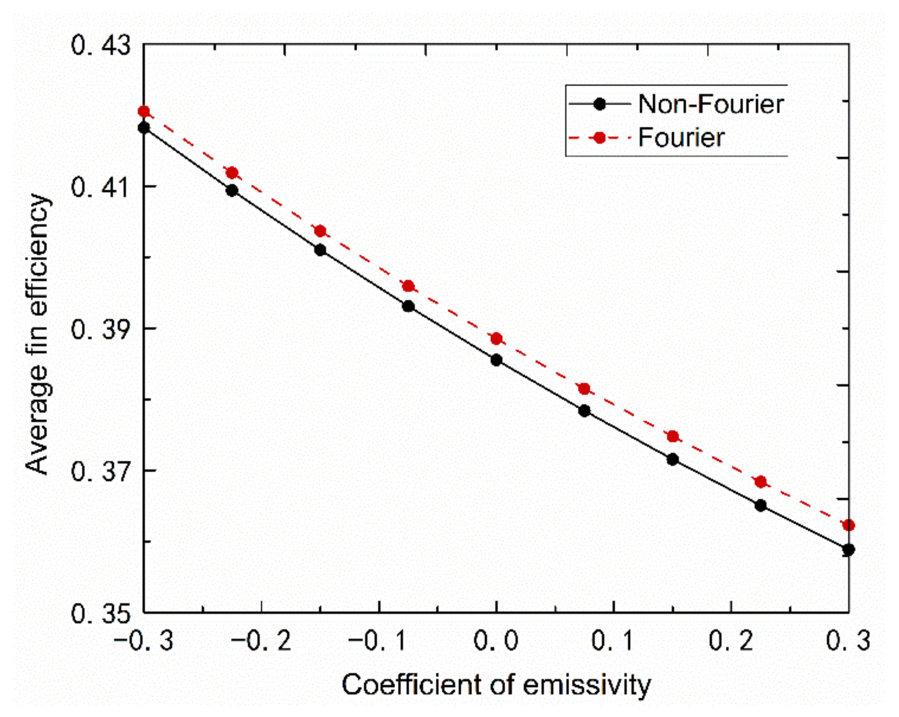
5.4. The Effect of Coefficient of Emissivity

Figure 13 and Figure 14 illustrate the effect of ξ on transient thermal behaviors of dimensionless fin tip temperature and fin efficiency. As shown in Figure 13, there is a negative correlation between the wave amplitude of dimensionless fin tip temperature and ξ. Both Fourier and non-Fourier models have the same change tendency. As shown in Figure 14, the wave amplitude of instantaneous fin efficiency becomes smaller when ξ increases from −0.3 to 0.3.
Figure 15 exhibits the variation of average fin efficiency with ξ for both Fourier and non-Fourier models. It is noted that average fin efficiency decreases with the increase of ξ. The relaxation time of the non-Fourier model is not zero. However, for the Fourier model, the relation time is zero. The Fourier model has a rapid temperature response speed and more heat dissipation through the fin. Thus, for the same emissivity, the fin efficiency of the Fourier model is higher than that of the non-Fourier model.

6. Conclusions

The element differential method was firstly developed to analyze non-Fourier heat conduction in convective-radiative fin with mixed boundary conditions. In the solving process, the derived spatial derivatives can be directly substituted into governing equations to form algebraic equations, and no mathematical principles or integration are required. The effects of various thermophysical parameters on dimensionless temperature, instantaneous fin efficiency, and average fin efficiency are also investigated. Based on the present study, the following conclusions can be drawn:
  • Comparison with analytical results and numerical method results in the literature shows that the element differential method is a convenient and straightforward method for solving nonlinear heat transfer of convective-radiative fin under the Fourier and non-Fourier models.
  • At the initial stage, the distribution of dimensionless temperature is very steep, and this phenomenon becomes more evident with the increase of Ve. As the dimensionless time goes on, the fluctuation of dimensionless temperature tends to stable, and the stable time is delayed as Ve increases.
  • The transient distribution of dimensionless fin tip temperature for the non-Fourier model has lag phenomena compared with that for the Fourier model. With the increase of Ve, the lag phenomena tend to be more obvious.
  • The wave amplitudes of dimensionless fin tip temperature and instantaneous fin efficiency become smaller when Ve, Ω, and ξ increase. In contrast, these opposite trends are found as b, μ, C1, C2, C3, and C4.
  • Average fin efficiency increases with the increase of μ, C1, C2, C3, and C4. However, average fin efficiency decreases with the increase of ξ. Otherwise, the fin efficiency of the Fourier model is higher than that of the non-Fourier model.

Author Contributions

Conceptualization, J.M. and Y.S.; methodology, J.M. and S.L.; software, S.L.; validation, J.M., Y.S. and S.L.; investigation, J.M.; data curation, S.L.; writing—original draft preparation, J.M.; writing—review and editing, Y.S. All authors have read and agreed to the published version of the manuscript.

Funding

This research was funded by National Natural Science Foundation of China (grant numbers 51976014, 51976173), and Natural Science Foundation of Jiangsu Province (grant number BK20201204).

Institutional Review Board Statement

Not applicable.

Informed Consent Statement

Not applicable.

Data Availability Statement

Not applicable.

Conflicts of Interest

The authors declare no conflict of interest.

Nomenclature

Acthe cross-section area of the fin, m2
Acoefficient matrix
Bamplitude of the input temperature
bpower index of convective heat transfer coefficient
C 1 , C 2 , C 3 , C 4 dimensionless coefficients of internal heat generation
c 1 , c 2 , c 3 , c 3 coefficients of internal heat generation
c p specific heat capacity, J · kg 1 · K 1
d vectors in Equation (19)
F Fourier number
Δ F dimensionless time step
h convective heat transfer coefficient, W · m 2 · K 1
k thermal conductivity, W · m 1 · K 1
L i n Lagrange interpolation polynomials
L length of the fin, m
m iteration times
N number of collocation points
N c coefficient of fin
N r c radiative-conductive parameter
n F number of shared surfaces
n i n t number of interpolations
n f normal vector
p perimeter of longitudinal fin, m
p e heat source vibration period, s
q heat transfer rate, W · m 2
Q c convective heat transfer rate, W · m 2
q volumetric heat generation rate, W · m 3
q i n the input of heat on the boundary, W · m 2
t time, s
T temperature, K
v speed of heat wave, m · s 1
V e Vernotte number
X dimensionless axial coordinate
x coordinate in the x-direction, m
Greek Symbols
α thermal diffusivity, m · s 1
δ thickness of the fin, m
ε surface emissivity
η instantaneous fin efficiency
η a v e average fin efficiency
μ coefficient of thermal conductivity
Θ dimensionless temperature
ξ coefficient of emissivity
ρ density, Kg · m 3
σ Stefan-Boltzmann constant, W · m 2 · K 4
τ relaxation time, s
χ dimensionless coordinate
Ω dimensionless periodicity
ω periodicity, s 1
Subscripts
i iteration times
value at ambient temperature
bvalue at fin base
i, jsolution node indexes
tvalue at the fin tip
Superscripts
m time level
f shared plane

References

  1. Liu, Y.; Li, L.; Zhang, Y.W. Numerical simulation of non-Fourier heat conduction in fins by lattice Boltzmann method. Appl. Therm. Eng. 2020, 166, 114670. [Google Scholar] [CrossRef]
  2. Cattaneo, C. A form of heat conduction equations which eliminates the paradox of instantaneous propagation. Comptes Rendus 1958, 247, 431–433. [Google Scholar]
  3. Vernotte, P. Some possible complications in the phenomena of thermal conduction. Comptes Rendus 1961, 252, 2190–2191. [Google Scholar]
  4. Eslinger, R.G.; Chung, B.T.F. Periodic heat transfer in radiating and convecting fins or fin arrays. AIAA J. 1979, 17, 1134–1140. [Google Scholar] [CrossRef]
  5. Lin, J.Y. The non-Fourier effect on the fin performance under periodic thermal conditions. Appl. Math. Model. 1998, 22, 629–640. [Google Scholar] [CrossRef] [Green Version]
  6. Das, R.; Mishra, S.C.; Kumar, T.B.P.; Uppaluri, R. An inverse analysis for parameter estimation applied to a non-Fourier conduction-radiation problem. Heat Transf. Eng. 2011, 32, 455–466. [Google Scholar] [CrossRef]
  7. Zahra, K.; Masoud, K.K.; Amir, O. Numerical study into the fin performance subjected to different periodic base temperatures employing Fourier and non-Fourier heat conduction models. Int. Commun. Heat Mass Transf. 2020, 114, 104562. [Google Scholar]
  8. Ndlovu, P.L.; Moitsheki, R.J. Steady state heat transfer analysis in a rectangular moving porous fin. Propuls. Power Res. 2020, 9, 188–196. [Google Scholar] [CrossRef]
  9. Das, R.; Kundu, B. Forward and inverse nonlinear heat transfer analysis for optimization of a constructal T-shape fin under dry and wet conditions. Int. J. Heat Mass Transf. 2019, 137, 461–475. [Google Scholar] [CrossRef]
  10. Torabi, M.; Zhang, Q.B. Analytical solution for evaluating the thermal performance and efficiency of convective-radiative straight 422 fins with various profiles and considering all non-linearities. Energy Conv. Manag. 2013, 66, 199–210. [Google Scholar] [CrossRef]
  11. Wankhade, P.A.; Kundu, B.; Das, R. Establishment of non-Fourier heat conduction model for an accurate transient thermal response in wet fins. Int. J. Heat Mass Transf. 2018, 126, 911–923. [Google Scholar] [CrossRef]
  12. Das, R.; Kundu, B. Direct and inverse approaches for analysis and optimization of fins under sensible and latent heat load. Int. J. Heat Mass Transf. 2018, 124, 331–343. [Google Scholar] [CrossRef]
  13. Mehraban, M.; Khosravi, N.M.R.; Shaahmadi, F. Thermal behavior of convective-radiative porous fins under periodic thermal conditions. Can. J. Chem. Eng. 2019, 97, 821–828. [Google Scholar] [CrossRef]
  14. Gireesha, B.J.; Sowmya, G.; Macha, M. Temperature distribution analysis in a fully wet moving radial porous fin by finite element method. Int. J. Numer. Methods Heat Fluid Flow 2022, 32, 453–468. [Google Scholar] [CrossRef]
  15. Prakash, D.; Ragupathi, E.; Muthtamilselvan, M.; Abdalla, B.; Mdallal, Q.M.A. Impact of boundary conditions of third kind on nanoliquid flow and radiative heat transfer through asymmetrical channel. Case Stud. Therm. Eng. 2021, 28, 101488. [Google Scholar] [CrossRef]
  16. Alhussain, Z.A.; Renuka, A.; Muthtamilselvan, M. A magneto-bioconvective and thermal conductivity enhancement in nanofluid flow containing gyrotactic microorganism. Case Stud. Therm. Eng. 2021, 23, 100809. [Google Scholar] [CrossRef]
  17. Renuka, A.; Muthtamilselvan, M.; Doh, D.H.; Cho, G.R. Entropy analysis and nanofluid past a double stretchable spinning disk using homotopy analysis method. Math. Comput. Simul. 2020, 171, 152–169. [Google Scholar] [CrossRef]
  18. Zhou, L.; Lv, J.; Cui, M.; Peng, H.F.; Gao, X.W. A polygonal element differential method for solving two-dimensional transient nonlinear heat conduction problems. Eng. Anal. Bound. Elem. 2023, 146, 448–459. [Google Scholar] [CrossRef]
  19. Sun, Y.S.; Zhao, J.Z.; Li, Y.F.; Li, S.D.; Zhou, R.R.; Ma, J. Angular-spatial upwind element differential method for radiative heat transfer in a concentric spherical participating medium. Eng. Anal. Bound. Elem. 2022, 144, 19–30. [Google Scholar] [CrossRef]
  20. Cui, M.; Xu, B.B.; Lv, J.; Gao, X.W.; Zhang, Y.W. Numerical solution of multi-dimensional transient nonlinear heat conduction problems with heat sources by an extended element differential method. Int. J. Heat Mass Transf. 2018, 126, 1111–1119. [Google Scholar] [CrossRef]
  21. Torabi, M.; Zhang, K.L. Heat transfer and thermodynamic performance of convective-radiative cooling double layer walls with temperature-dependent thermal conductivity and internal heat generation. Energy Conv. Manag. 2015, 89, 12–23. [Google Scholar] [CrossRef]
  22. Chen, H.; Ma, J.; Liu, H.T. Least square spectral collocation method for nonlinear heat transfer in moving porous plate with convective and radiative boundary conditions. Int. J. Therm. Sci. 2018, 132, 335–343. [Google Scholar] [CrossRef]
  23. Singh, S.; Kumar, D.; Rai, K.N. Analytical solution of Fourier and non-Fourier heat transfer in longitudinal fin with internal heat generation and periodic boundary condition. Int. J. Therm. Sci. 2018, 125, 166–175. [Google Scholar] [CrossRef]
Figure 1. Physical model of the convective-radiative fin with mixed boundary conditions.
Coatings 12 01862 g001
Figure 2. Three kinds of nodes of isoparametric elements.
Coatings 12 01862 g002
Figure 3. Comparison of dimensionless temperature by the EDM and analytical solution.
Coatings 12 01862 g003
Figure 4. Comparison of dimensionless fin tip temperature by the EDM and the θ method [13].
Coatings 12 01862 g004
Figure 5. Dimensionless temperature for different values of Ve.
Coatings 12 01862 g005
Figure 6. The variation of instantaneous fin tip temperature for different values of Ve.
Coatings 12 01862 g006
Figure 7. The variation of instantaneous fin efficiency at different values of Ve.
Coatings 12 01862 g007
Figure 8. The variation of fin tip temperature at different values of Ω.
Coatings 12 01862 g008
Figure 9. The variation of instantaneous fin efficiency at different values of Ω.
Coatings 12 01862 g009
Figure 10. The variation of fin tip temperature at different values of μ.
Coatings 12 01862 g010
Figure 11. The variation of instantaneous fin efficiency at different values of μ.
Coatings 12 01862 g011
Figure 12. The variation of average fin efficiency with different values of μ.
Coatings 12 01862 g012
Figure 13. The variation of fin tip temperature at different values of ξ.
Coatings 12 01862 g013
Figure 14. The variation of instantaneous fin efficiency at different values of ξ.
Coatings 12 01862 g014
Figure 15. The variation of average fin efficiency with different values of ξ.
Coatings 12 01862 g015
Publisher’s Note: MDPI stays neutral with regard to jurisdictional claims in published maps and institutional affiliations.

