Article

Intelligent Metal Welding Defect Detection Model on Improved FAST-PNN

1
School of Medical Technology, Beihua University, Jilin 132000, China
2
School of Civil Engineering and Transportation, Beihua University, Jilin 132000, China
*
Author to whom correspondence should be addressed.
Coatings 2022, 12(10), 1523; https://doi.org/10.3390/coatings12101523
Submission received: 22 August 2022 / Revised: 21 September 2022 / Accepted: 8 October 2022 / Published: 11 October 2022
(This article belongs to the Special Issue Recent Progress in Metal Additive Manufacturing)

Abstract

:
In order to solve the problem of accurate and efficient detection of welding defects in the process of batch welding of metal parts, an improved Probabilistic Neural Network (PNN) algorithm was proposed to build an automatic identification model of welding defects. Combined with the characteristics of the PNN model, the structure and algorithm flow of the FAST-PNN algorithm model are proposed. Extraction of welding defect image texture features of metal welded parts by a Gray Level Co-occurrence Matrix (GLCM) screens out the characteristic indicators that can effectively characterize welding defects. Weld defect texture features are used as input to build a defect classification model with FAST-PNN, for accurate and efficient classification of welding defects. The results show that the improved FAST-PNN model can effectively identify the types of welding defects such as burn-through, pores and cracks, etc. The classification recognition accuracy and recognition efficiency have been significantly improved. The proposed defect welding identification method can accurately and effectively identify the damage types of welding defects based on a small number of defect sample images. Welding defects can be quickly identified and classified by simply collecting weld images, which helps to solve the problem of intelligent, high-precision, fast real-time online detection of welding defects in modern metal structures; it provides corresponding evidence for formulating response strategies, with a certain theoretical basis and numerical reference.

1. Introduction

Metal welding processing methods exist in various industries, aerospace, automobile manufacturing, shipbuilding, etc., and are all inseparable from welding. The welding process is affected by various parameters and the testing environment, resulting in various welding defects such as burn-through, porosity, cracks and lack of fusion in the welds of metal parts [1,2]. It is very difficult to accurately detect the weld seam of welded products in the actual industrial welding process. On the one hand, the investment is large, and on the other hand, the labor cost is high and the misjudgment rate is high. At the same time, the existence of welding defects seriously affects the service life of welded parts. Therefore, product post-weld inspection is an important issue that needs to be solved urgently [3,4,5,6].
Building a mathematical model according to the actual problem, solving the mathematical model and then solving the actual problem according to the results are widely used in various fields [7,8,9]. An artificial neural network is also a kind of mathematical modeling, which makes predictions after building models. With the wide application of intelligent welding defect detection instruments in engineering practice, how to accurately identify welding defects under complex constraints has become a research hotspot, and the existing research results demonstrate that the performance of welding defect recognition models based on artificial neural networks is particularly outstanding [10,11,12,13]. Welding defect recognition based on neural networks [14,15] involves selecting the parameters sensitive to defects as the input of the neural network, training the neural network through the defect data in the numerical simulation and finally applying the trained network to the detection of metal parts to realize the automatic identification of defects [16,17,18,19,20]. Ma et al. constructed a Convolutional Neural Network (CNN) to identify the spectrum graphs, realizing the online detection of porosity [21]. Gao et al. applied a deep CNN to identify welding defects obtained in different inspection environments, and obtained better inspection results [22]. Fan et al. carried out real-time classification and identification of laser welding defects using s CNN algorithm model and Auxiliary Classifier Generative Adversarial Network (ACGAN) model classification [23]. Amirafshari et al. predicted the Probability of Detection (POD) using Bayes’ theorem with commonly used hit/miss models, and estimated weld defect size and frequency [24]. Liu et al. proposed a class activation mapping method that fuses multi-scale features [25]. However, the complex constraints of the inspection environment impair the image quality, various defects on the welding surface seriously interfere with the inspection efficiency and the lack of sample space in the actual measurement site limits the establishment of an intelligent system for defects. This series of problems leads to the problem of reduced accuracy and prolonged testing waiting time in welding defect identification research [26,27,28]. Therefore, it is necessary to explore a fast and high-precision welding defect identification method that is more in line with on-site inspection.
A PNN is an algorithm based on the Bayes decision theory and parzen window probability density function, which is developed on the basis of a radial basis neural network [29,30,31]. Compared with other neural networks, the calculation process of a PNN is simple, the convergence speed is fast and the stability is high. The network has strong fault tolerance for individual abnormal data and, for newly added or deleted sample data, it can maintain a high classification accuracy without retraining. It can also meet the requirements of modification at any time during sample training. At present, PNNs are widely used in the field of fault diagnosis [32,33]. There are difficulties in welding defect damage identification research, metal materials are industrialized products and the degree of mechanization, automation and intelligence of infrastructure is low. The welding defect samples that can be extracted at this stage are extremely scarce, which seriously affects the identification accuracy of welding defects. Due to the network characteristics of a PNN, it can still maintain high recognition accuracy under the condition of a small amount of sample data. However, the traditional PNN model is limited by the network structure, and the recognition efficiency is generally low, which cannot meet the current requirements for efficient and fast detection of welding defects. Therefore, this paper improves the traditional PNN model structure and learning algorithm, and proposes a FAST-PNN model.
The research object of this paper is pictures of weld defects of CO2 gas shielded arc welding. The steps involve obtaining welding defect images using an image acquisition system; selecting digital image processing techniques to optimize image quality in the inspection area; extracting the characteristic parameters of welding defects through image texture analysis technology, and establishing a standard sample database for identifying welding defect images. We build a FAST-PNN model for welding defect classification and identification, gaining higher identification accuracy in a limited sample of weld defects. The validity of the improved model is verified based on the recognition accuracy of detection samples and test samples.

2. Method

2.1. Gray Level Co-Occurrence Matrix (GLCM)

Weld defect images are varied and extremely complex. A GLCM based on statistical theory meets the actual detection conditions by adjusting three important construction factors (gray level g, generation step d and generation direction θ). Based on the GLCM, 14 characteristic parameters can be extracted to quantify the texture characteristics of welding defects in a multi-dimensional and all-round way. Taking the screened feature parameters as standard and the sample as the input of the network model, a PNN model of welding defects with low demand for samples and high recognition accuracy can be constructed.
The GLCM starts from the pixel (x, y) whose gray value is i, and counts the pixel (x + a, y + b) whose distance is d and whose gray value is j, and the probability of simultaneous occurrence is mathematically expressed as:
P i , j , d , θ [ x , y , x + a , y + b | f x , y = i ; f x + a , y + b = j ] .
Among them, the value range of i, j determines the image gray level g, d is the generation step size; θ is the generation direction of the GLCM, usually taking four growth directions of 0°, 45°, 90° and 135°.

2.2. Construction Factor

The image gray level g, the generation step size d and the generation angle θ are the three construction factors of the GLCM, which together determine the conditional criteria for generating the GLCM. The form of the GLCM generated under the criterion determines the reliability of the extracted feature parameters.
(1)
The image grayscale of g
The image gray level g determines the size of the grayscale co-occurrence matrix of the welding defect image and is an important parameter to measure the quality of the welding defect image.
(2)
The generation step size of d
The generation step d is used as the connection distance between the center positions of the pixel points of the defect image in the process of constructing the gray level co-occurrence matrix of the welding defect image. The generation step size d is set based on the distance between the welding defect texture primitive and the primitive. Weld defect primitives are finely textured with small d values, weld defect texture primitives are coarse textured with large d values.
(3)
The generation direction of θ
The generation direction θ is the angle between the two pixels of the welding defect image, that is, the angle between the initial defect pixel and the end defect pixel according to the counterclockwise direction, taking 0°, 45°, 90°, 135°. This is because the welding defect image texture base element and the base element constitute a certain angle. Therefore, it is very important to choose the appropriate generation direction to describe the defect texture.

2.3. Characteristic Parameters

The grayscale matrix of the image reflects the visual information of the image, and the GLCM reflects the comprehensive information of the image grayscale on the direction, adjacent interval and variation range. The local pattern and arrangement rules of the image can be analyzed by the GLCM, but generally not the co-occurrence matrix obtained by direct application, but the secondary statistics are obtained on the basis of it. Before obtaining the characteristic parameters of the GLCM, it is necessary to perform normalization processing:
P i , j , d , θ = P i , j , d , θ / R .
Among them, R is the normalization constant, and is the sum of all elements in the GLCM.
Haralick et al. defined 14 GLCM feature parameters for texture analysis [34], and the characteristic parameters and their calculation formulas are shown in Table 1.
In the formula, u 1 = i = 1 g i j = 1 g p i , j , d , θ , u 2 = i = 1 g j j = 1 g p i , j , d , θ , d 1 2 = i = 1 g ( i u 1 ) 2 j = 1 g p i , j , d , θ , d 2 2 = j = 1 g ( j u 1 ) 2 i = 1 g p i , j , d , θ ; P X k = i = 1 g j = 1 g p i , j , d , θ i + j = k k = 2 , 3 , 2 g ; P Y k = i = 1 g j = 1 g p i , j , d , θ i j = k k = 2 , 3 , 2 g ; m is the mean of p i , j , d , θ .
It can be seen from Table 1 that the 14 characteristic parameters are related to the combination of construction factors, different combinations will generate different GLCMs, resulting in different feature parameters, and the obtained feature parameters will express different textures. The main tool for analyzing textures is texture feature parameters. Therefore, in this study, from the perspective of characteristic parameters, the GLCM construction method suitable for welding defect texture was determined.

2.4. Fast Probabilistic Neural Network

In the process of welding defect identification, the extracted feature vector is usually used as the input, and the output is the probability of the category. In order to improve the performance of the welding defect recognition network model, the network structure is improved, and the improved PNN model is shown in Figure 1.
The improved PNN is a feedforward neural network with multiple parzen windows. The structure is divided into 4 layers, namely input layer, pattern layer, summation layer and output layer. As shown Figure 1, the improved output layer consists of a planar array.

2.5. Fast Probabilistic Neural Network Algorithm (FAST-PNN)

The traditional PNN model, its output layer is one-dimensional. The improved PNN (FAST-PNN) optimizes its output layer from a traditional one-dimensional output layer to a two-dimensional output surface and defines a neighborhood window. Its network process is as follows: the input layer of the FAST-PNN is used as the input of the feature vector, and the feature vector is passed to the next layer of the network to normalize the input samples. The core key of the FAST-PNN model is to establish a neighborhood window in the output array to quickly detect the category of multiple output neurons. The specific algorithm steps are as follows:
(1)
Determination of input vector: The input feature vector of the data sample is passed to the FAST-PNN network, that is, the feature vector X calculated by the GLCM processing is used as the input of the FAST-PNN. Since the number of neuron nodes in the input layer in FAST-PNN is equal to the dimension of the input vector, the input layer of the network contains n neuron nodes.
(2)
Establishment of radial base: The radial base layer kernel function is a Gaussian function. The number of neuron nodes in this layer is the same as the number of input training samples. It directly stores the training samples as the pattern vector of the network and calculates the radial basis of each input vector and mode vector when classifying the data, so as to obtain an estimate of the density function of the input vector.
(3)
Calculation of the summation layer: The number of neurons in the summation layer is the same as the data pattern category. Each node is only connected to the neurons of the corresponding mode category in the radial base layer, and the probability estimates under each mode are summed and averaged.
(4)
Determination of the output layer: The output layer sets the pattern output with the largest posterior probability to 1 and the rest to 0, thus realizing pattern prediction classification.
(5)
Establishment of the neighborhood window: The neighborhood shape and the neighborhood radius are determined according to the output layer array and the number of categories. The neuron and its neighboring neuron categories are determined, the window slides until all the output layer arrays are judged and the process ends.

3. Test and Result Analysis

The working steps of a welding defect recognition model based on the combination of a GLCM and probabilistic neural network are shown in Figure 2.
According to Figure 2, it can be seen that the recognition and classification of welding defect patterns based on a GLCM and FAST-PNN are divided into three core steps: image processing, feature parameter extraction and screening and network construction. First, acquire and process welding defect images and analyze the texture characteristics of welding defects. Then, extract and screen the characteristic parameters of the welding defect image to construct a parameter set. Finally, a welding defect recognition model is constructed based on the improved FAST-PNN, the pattern vector density function is used to calculate its probability, the probability is summed and then the average value is calculated. Design the output layer neighborhood window, slide the neighborhood window until the welding defect types of all neurons are output and end the process.

3.1. Image Acquisition and Processing

The complex defect types on the welding surface and the existence of many unfavorable factors in the inspection environment seriously interfere with inspection, such as light, welding fumes, oil on the surface of welding parts, etc. In order to provide high-quality sample labels, Digital Image Processing (DIP) technology is applied to optimize image quality, remove noise information that affects image quality, such as light, welding smoke and image transmission, reduce redundant information and obtain images of defective areas. The welding-related parameters of the target weld are obtained as shown in Table 2. The welding picture of the assembly obtained by the target weld is shown in Figure 3.
Each weldment in Figure 3 is welded by multiple welds and, during the mass production process, different types of welding defects will occur. A Nikon-d850 (Nikon, Tokyo, Japan) was used to build a welding defect image acquisition system (30–40 cm away from the weld, perpendicular to the weld), and 150 target weld surface defect images were randomly collected. The region of interest was extracted sequentially, followed by grayscale transformation, histogram equalization and median filtering. Figure 4 is the grayscale image of five kinds of welding defects after processing. In order to better distinguish between normal and defective welds, we also incorporate normal welds into the target welds for weld detection and identification, which is more conducive to engineering practice applications.
We contrast and analyze the information contained in each grayscale image in Figure 4. The images have the advantages of clear texture, clear defect target and strong overall contrast. Different types of welding defect texture images each show unique linear texture primitives, and the uniformity and randomness of texture distribution are different. Therefore, the characteristic parameters of each defect can be extracted according to the texture analysis method as the standard sample of the welding defect identification network model.

3.2. Feature Parameter Extraction and Screening

The characteristic parameters of each defect image were extracted based on GLCM, and the construction factor was determined as follows: generation step size d = 1, image gray level g = 256, the generation direction θ takes 0°, 45°, 90°, 135°. Under this construction factor, a GLCM suitable for characterizing defect image information was constructed. The matrix was normalized and all feature parameters were extracted. In order to extract more representative parameters and obtain higher defect recognition accuracy in a limited sample space, 6 characteristic parameters were screened out, to establish high-quality standard samples, as shown in Table 3.

3.3. Standard Sample Establishment

In order to accurately extract defect information, crack, burn-through, porosity, non-fused and normal images were selected, and the average value of their characteristic parameters as the standard sample value was obtained. The angular second moment is denoted as X1, contrast as X2, entropy as X3, variance as X4, correlation as X5 and clustering shadow as X6. Table 4 shows the standard sample parameter values corresponding to each defect.
We contrast and analyze the fluctuations of the parameter values in Table 4, and build a standard set in a specific interval from X1 to X6, which can be used as an evaluation standard for effectively distinguishing defect types.

3.4. Network Model Building

A Nikon-d850 (Nikon, Tokyo, Japan) was used to obtain five kinds of welding defect images, and the welding defect images were processed. Figure 4 shows the process of image acquisition.
Based on the method shown in Figure 5, 70 images of each welding defect were collected and processed. The processed 50 images were taken as training samples and 20 as test samples. The feature parameters were extracted by the gray level co-occurrence matrix as the input pattern set of the PNN model, and the standard sample vector of welding defect types is formed:
X = X 1 , X 2 , X 3 , X 4 , X 5 , X 6
The feature dimension is 6, the number of training samples for each welding defect is 50 and there are 1500 sample data in total. Then, there are:
X = x 11 x 12 x 13 x 14 x 15 x 16 x 21 x 21 x 21 x 24 x 25 x 26 x 2501 x 2502 x 2503 x 2504 x 2505 x 2506 250 × 6
The total energy of the eigenvectors of the PNN model of welding defects is calculated, denoted as matrix A, then:
A = 1 i = 1 6 x 2 1 i 1 i = 1 6 x 2 2 i 1 i = 1 6 x 2 3 i 1 i = 1 6 x 2 250 i 1 × 250
After normalizing the welding defect samples, matrix B is obtained:
B = 1 1 1 1 1 250 × 1   A     x 11 x 12 x 13 x 14 x 15 x 16 x 21 x 21 x 21 x 24 x 25 x 26 x 2501 x 2502 x 2503 x 2504 x 2505 x 2506 250 × 6 = [ x 11 i = 1 250 x 2 1 i x 12 i = 1 250 x 2 2 i x 13 i = 1 250 x 2 3 i x 14 i = 1 250 x 2 4 i x 15 i = 1 250 x 2 5 i x 16 i = 1 250 x 2 6 i x 11 i = 1 250 x 2 1 i x 12 i = 1 250 x 2 1 i x 13 i = 1 250 x 2 1 i x 14 i = 1 250 x 2 4 i x 15 i = 1 250 x 2 5 i x 16 i = 1 n x 2 6 i x 11 i = 1 250 x 2 1 i x 12 i = 1 250 x 2 1 i x 13 i = 1 250 x 2 1 i x 14 i = 1 250 x 2 4 i x 15 i = 1 250 x 2 5 i x 16 i = 1 n x 2 6 i ] 250 × 6 = C 11 C 12 C 13 C 14 C 15 C 16 C 21 C 21 C 21 C 14 C 15 C 26 C 2501 C 2502 C 2503 C 2504 C 2505 C 2506 250 × 6
The normalized sample data C 250 × 6 of the input end is input into the pattern layer, the pattern layer is only connected to the summation layer corresponding to the same defect category and the others do not interfere with each other. There are a total of 5 types of welding defects in our welding defect category, and there are 50 of each type of sample data, then the total number of neurons in the mode layer is 250, and the neurons in the mode layer correspond to the same type of input sample data, that is, 1~50 neurons in the mode layer represent the first type of welding defect, 51~100 neurons represent the second type of welding defect, 101~150 neurons represent the third type of welding defect, 151~200 neurons represent the fourth type of welding defect, 201~250 neurons represent the fifth type of welding defect. The pattern layer calculates the Euclidean distance between the input normalized feature vector and the training samples of the summation layer, and multiplies the pattern layer vector with the corresponding threshold. Finally, the Gaussian function activation is used to obtain the probability of the corresponding mode.
In the prediction of welding defect pattern samples based on a probabilistic neural network, the number of defect pattern test samples is 25, and matrix D composed of 25 6-dimensional vectors is used to calculate the Euclidean distance among the samples to be identified and the training samples:
E i , j = D i C j D i C j T 1 2 = k = 1 6 d i k c i k 2
The Gaussian function is used to activate, taking the variance as:
E = [ e k = 1 30 | d 1 i c 1 i | 2 2 σ 2 e k = 1 30 | d 1 i c 2 i | 2 2 σ 2 e k = 1 30 | d 1 i c 30 i | 2 2 σ 2 e k = 1 30 | d 2 i c 1 i | 2 2 σ 2 e k = 1 30 | d 2 i c 2 i | 2 2 σ 2 e k = 1 30 | d 2 i c 30 i | 2 2 σ 2 e k = 1 30 | d 25 i c 1 i | 2 2 σ 2 e k = 1 30 | d 25 i c 2 i | 2 2 σ 2 e k = 1 30 | d 25 i c 30 i | 2 2 σ 2 ] 25 × 30 = E 11 E 12 E 130 E 21 E 22 E 230 E 251 E 252 E 2530 25 × 30
That is, the output probability of the mode layer can be expressed as F:
F = h = 1 6 E 1 h h = 7 12 E 1 h h = 13 18 E 1 h h = 19 24 E 1 h h = 25 30 E 1 h h = 1 6 E 2 h h = 7 12 E 2 h h = 13 18 E 2 h h = 19 24 E 2 h h = 25 30 E 2 h h = 1 6 E 25 h h = 7 12 E 25 h h = 13 18 E 25 h h = 19 24 E 25 h h = 25 30 E 25 h 25 × 30
The summation layer neuron obtains the initial probability sum of the pattern layer and calculates the estimated probability of the welding defect category of the sample to be identified and the output layer neuron receives the initial probability of various welding defect categories input from the summation layer. According to the Bayes rule, the input sample to be tested is divided into the welding defect types with the maximum posterior probability, and the input sample X is mathematically described as:
h 1 l 1 F i 1 X > h i l i F i r X   r 1 ,   then   X ( 1   0   0   0   0 ) h 2 l 2 F i 2 X > h i l i F i r X   r 2 ,   then   X ( 0   1   0   0   0 ) h 3 l 3 F i 3 X > h i l i F i r X   r 3 ,   then   X ( 0   0   1   0   0 ) h 4 l 4 F i 4 X > h i l i F i r X   r 4 ,   then   X ( 0   0   0   1   0 ) h 5 l 5 F i 5 X > h i l i F i r X   r 5 ,   then   X ( 0   0   0   0   1 )
Among them: h 1 = N 1 N ,   h 2 = N 2 N ,   h 3 = N 3 N ,   h 4 = N 4 N ,   h 5 = N 5 N .
In the formula, h 1 ,   h 2 ,   h 3 , h 4 and h 5 are the prior probabilities of modes 1, 2, 3, 4 and 5, l 1 ,   l 2 ,   l 3 ,   l 4 and l 5 are the cost factors for fault judgment errors, f 1 ,   f 2 ,   f 3 ,   f 4 and f 5 are the probability density functions of five welding defects. N 1 ,   N 2 ,   N 3 ,   N 4 and N 5 are the number of samples for each type of welding defect, N is the total number of samples.
According to the number of welding defect neurons and the type of welding defect, the output array hexagonal neighborhood window is selected, and the neighborhood radius d = 1. The output layer obtains the maximum probability density function neuron, and its output is 1, that is, 1   0   0   0   0 , 0   1   0   0   0 , 0   0   1   0   0 , 0   0   0   1   0 and 0   0   0   0   1 represent cracks, burn-through, pore, not fused and normal, respectively.

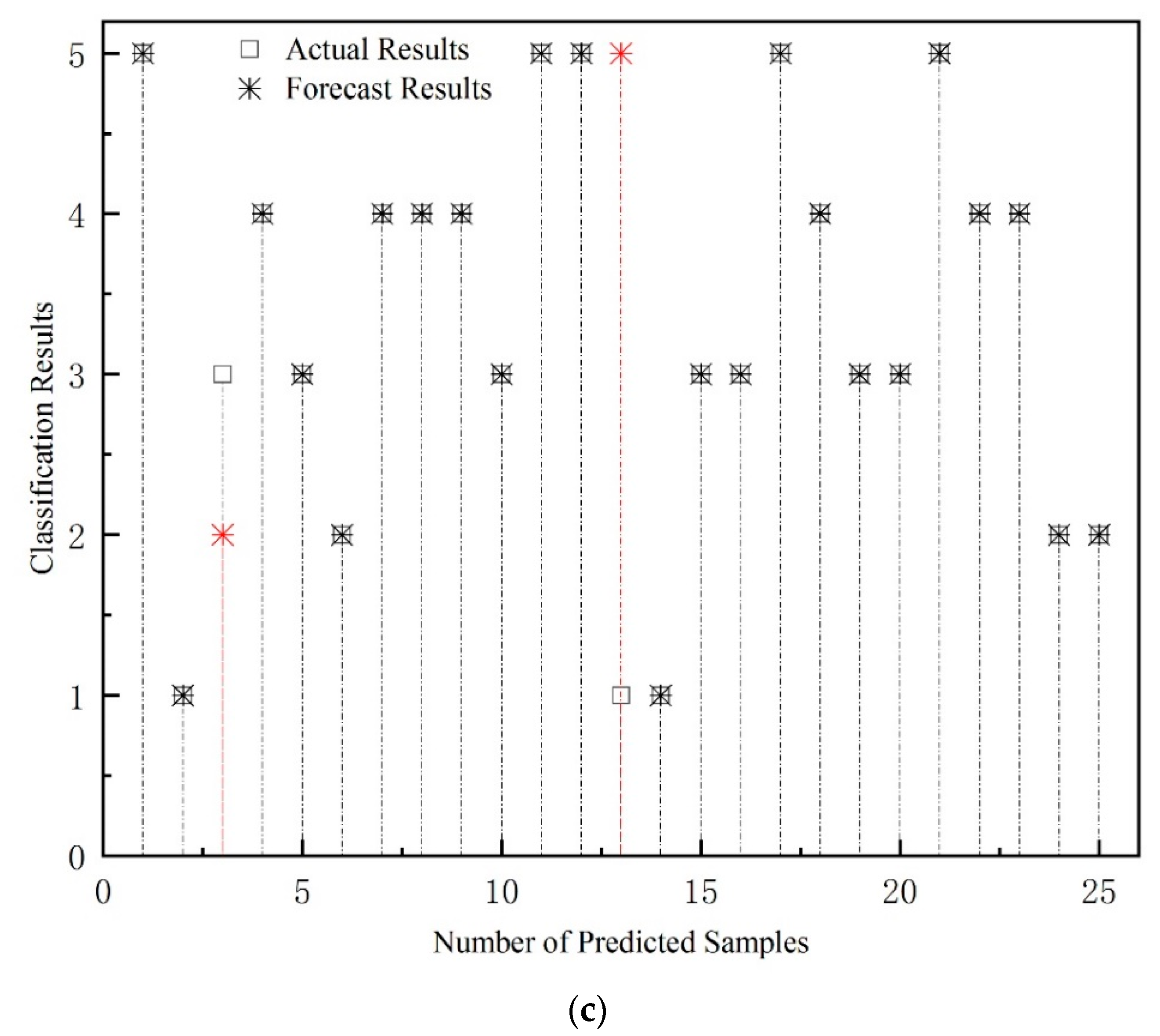
3.5. Result Analysis

Combined with the above FAST-PNN model, the feature parameters extracted from 250 defect sample pictures are processed and input into the network. Due to the large amount of data, the output data graph cannot be fully displayed, and Figure 6 only shows the renderings of 75 groups of training samples and their error maps after training.
It can be seen from Figure 6a,b that, after training, 75 sets of training data were taken as input into the trained PNN, only five samples were judged incorrectly and the accuracy rate reached 93.33%. At the same time, comparing FAST-PNN with the traditional PNN model, it is found that the recognition accuracy remains unchanged, and the recognition consumption time is shortened. For the same 75 sets of data, the traditional PNN identification took about 274 s, while the FAST-PNN identification took about 204 s, so the efficiency is increased by 27.54%. Using the trained FAST-PNN, 25 sets of test data were input to check the predicted effect of the neural network, and the result is shown in Figure 6c, in which the squares represent the actual classification results, and the asterisks represent the predicted classification results. As can be seen from Figure 6c, among the 25 sets of prediction samples, only one set of test samples is wrong, with an accuracy rate of 96%, and the efficiency is 25.48% higher than the traditional model. Therefore, FAST-PNN can be used in welding defect pattern classification.

4. Conclusions

A welding defect identification method combining improved PNN and texture analysis technology is proposed, which can effectively eliminate the interference of environmental factors based on limited sample space (about 70 pieces for each defect), obtain higher welding defect identification accuracy and effectively improve the network identification efficiency. The following conclusions were reached:
(1)
Based on image processing methods such as grayscale transformation, regional image interception, histogram equalization and median filtering, the interference of environmental factors is removed, and defect images with clear targets and strong contrast are obtained. Combined with the gray level co-occurrence matrix, the texture feature parameter set (angular second moment, entropy, etc.) is screened out, and the standard sample of the network model is established.
(2)
By adjusting various parameters of the network, the welding defect recognition model of FAST-PNN is constructed. Based on FAST-PNN, five kinds of welding defects, including cracks, burn-through, porosity, non-fusion and normal defects, are predicted and classified, the accuracy rate reaches 93.33% and the efficiency of network identification has been significantly improved.
In engineering practice, welding defects exist in real time. The research method in this paper can quickly identify weld defects by simply obtaining weld pictures, and can quickly classify and provide corresponding evidence to formulate coping strategies, which has a certain theoretical basis and numerical reference.

Author Contributions

Conceptualization, J.L. and K.L.; Data curation, J.L. and K.L.; Formal analysis, J.L.; Funding acquisition, J.L. and K.L.; Investigation, J.L.; Methodology, J.L. and K.L.; Project administration, J.L.; Resources, J.L. and K.L.; Software, J.L. and K.L.; Supervision, K.L.; Validation, K.L.; Visualization, J.L.; Writing—original draft, Jinxin Liu; Writing—review and editing, J.L. and K.L. All authors have read and agreed to the published version of the manuscript.

Funding

This research was funded by PhD research start-up project of Beihua University, grant number 160321009.

Institutional Review Board Statement

Not applicable.

Informed Consent Statement

Not applicable.

Data Availability Statement

Not applicable.

Conflicts of Interest

The authors declare no conflict of interest.

References

  1. Zhang, H.; Jiang, M.; Chen, X.; Wei, L.; Wang, S.; Jiang, Y.; Jiang, N.; Wang, Z.; Lei, Z.; Chen, Y. Investigation of weld root defects in high-power full-penetration laser welding of high-strength steel. Materials 2022, 15, 1095. [Google Scholar] [CrossRef] [PubMed]
  2. Alvarenga, T.A.; Carvalho, A.L.; Honorio, L.M.; Cerqueira, A.S.; Filho, L.M.; Nobrega, R.A. Detection and classification system for rail surface defects based on Eddy current. Sensors 2021, 21, 7937. [Google Scholar] [CrossRef] [PubMed]
  3. Valdiande, J.J.; Rodriguez-Cobo, L.; Cobo, A.; Lopez-Higuera, J.M.; Mirapeix, J. Spectroscopic approach for the on-line monitoring of welding of tanker trucks. Appl. Sci. 2022, 12, 5022. [Google Scholar] [CrossRef]
  4. Li, Y.; Xu, F. Structural damage monitoring for metallic panels based on acoustic emission and adaptive improvement variational mode decomposition–wavelet packet transform. Struct. Health Monit. 2021, 21, 710–730. [Google Scholar] [CrossRef]
  5. Ettefagh, M.M. Damage identification of a TLP floating wind turbine by meta-heuristic algorithms. China Ocean. Eng. 2022, 29, 891–902. [Google Scholar] [CrossRef]
  6. Gao, Y.; Zhong, P.; Tang, X.; Hu, H.; Xu, P. Feature extraction of laser welding pool image and application in welding quality identification. IEEE Access 2021, 9, 120193–120202. [Google Scholar] [CrossRef]
  7. Dhanesh Babu, S.D.; Sevvel, P.; Senthil Kumar, R.; Vijayan, V.; Subramani, J. Development of thermo mechanical model for prediction of temperature diffusion in different FSW tool pin geometries during joining of AZ80A Mg alloys. J. Inorg. Organomet. Polym. Mater. 2021, 31, 3196–3212. [Google Scholar] [CrossRef]
  8. Thangaiah, S.I.; Sevvel, P.; Satheesh, C.; Mahadevan, S. Experimental study on the role of tool geometry in determining the strength & soundness of wrought Az80a Mg alloy joints during FSW process. FME Trans. 2018, 46, 612–622. [Google Scholar]
  9. Babu, S.D.D.; Sevvel, P.; Kumar, R.S. Simulation of heat transfer and analysis of impact of tool pin geometry and tool speed during friction stir welding of AZ80A Mg alloy plates. J. Mech. Sci. Technol. 2020, 34, 4239–4250. [Google Scholar] [CrossRef]
  10. Madhvacharyula, A.S.; Pavan, A.V.S.; Gorthi, S.; Chitral, S.; Venkaiah, N.; Kiran, D.V. In situ detection of welding defects: A review. Weld. World 2022, 66, 1–18. [Google Scholar] [CrossRef]
  11. Liu, W.; Shan, S.; Chen, H.; Wang, R.; Sun, J.; Zhou, Z. X-ray weld defect detection based on AF-RCNN. Weld. World 2022, 66, 1–13. [Google Scholar] [CrossRef]
  12. Xu, H.; Yan, Z.H.; Ji, B.W.; Huang, P.F.; Cheng, J.P.; Wu, X.D. Defect detection in welding radiographic images based on semantic segmentation methods. Measurement 2022, 188, 110569. [Google Scholar] [CrossRef]
  13. Yu, H.; Yin, J.; Li, Y. Gate attentional factorization machines: An efficient neural network considering both accuracy and speed. Appl. Sci. 2021, 11, 9546. [Google Scholar] [CrossRef]
  14. Zhu, C.; Yuan, H.; Ma, G. An active visual monitoring method for GMAW weld surface defects based on random forest model. Mater. Res. Express 2022, 9, 036503. [Google Scholar] [CrossRef]
  15. Wei, L.; Liang, T. Pattern recognition algorithm of welding defects in digital radiographic images. Value Eng. 2015, 34, 115–119. [Google Scholar]
  16. Melakhsou, A.A.; Batton-Hubert, M. Welding monitoring and defect detection using probability density distribution and functional nonparametric kernel classifier. J. Intell. Manuf. 2021, 1–13. [Google Scholar] [CrossRef]
  17. Yang, L.; Wang, H.; Huo, B.; Li, F.; Liu, Y. An automatic welding defect location algorithm based on deep learning. NDT E Int. 2021, 120, 102435. [Google Scholar] [CrossRef]
  18. Xu, Z.; Wu, M.; Fan, W. Sparse-based defect detection of weld feature guided waves with a fusion of shear wave characteristics. Measurement 2021, 174, 109018. [Google Scholar] [CrossRef]
  19. Miao, R.; Shan, Z.; Zhou, Q.; Wu, Y.; Ge, L.; Zhang, J.; Hu, H. Real-time defect identification of narrow overlap welds and application based on convolutional neural networks. J. Manuf. Syst. 2022, 62, 800–810. [Google Scholar] [CrossRef]
  20. Ban, G.; Yoo, J. RT-SPeeDet: Real-time IP–CNN-based small pit defect detection for automatic film manufacturing inspection. Appl. Sci. 2021, 11, 9632. [Google Scholar] [CrossRef]
  21. Ma, D.; Jiang, P.; Shu, L.; Geng, S. Multi-sensing signals diagnosis and CNN-based detection of porosity defect during Al alloys laser welding. J. Manuf. Syst. 2022, 62, 334–346. [Google Scholar] [CrossRef]
  22. Gao, X.; Lan, C.; Chen, Z.; You, D.; Li, G. Dynamic detection and identificationof welding defects by magneto-optical imaging. Opt. Precis. Eng. 2017, 25, 1135–1141. [Google Scholar]
  23. Fan, K.; Peng, P.; Zhou, H.; Wang, L.; Guo, Z. Real-time high-performance laser welding defect detection by combining ACGAN-based data enhancement and multi-model fusion. Sensors 2021, 21, 7304. [Google Scholar] [CrossRef] [PubMed]
  24. Amirafshari, P.; Kolios, A. Estimation of weld defects size distributions, rates and probability of detections in fabrication yards using a Bayesian theorem approach. Int. J. Fatigue 2022, 159, 106763. [Google Scholar] [CrossRef]
  25. Liu, T.; Zheng, H.; Yang, C.; Bao, J.; Wang, J.; Gu, J. Explainable deep learning method for laser welding defect recognition. Acta Aeronaut. Astronaut. Sinica 2022, 43, 10. (In Chinese) [Google Scholar]
  26. Ji, Y.; Gao, X.; Liu, Q.; Zhang, Y.; Zhang, N. Recognition method of welding defect magneto-optical imaging convolutional neural network. J. Instrum. Instrum. 2021, 42, 107–113. [Google Scholar]
  27. Gong, J.; Li, H.; Li, L.; Wang, G. Quality monitoring technology of laser welding process based on coaxial image sensing. J. Weld. 2019, 40. (In Chinese) [Google Scholar] [CrossRef]
  28. Lan, C.; Gao, X.; Ma, N.; Zhang, N. Texture feature extraction and recognition of magneto-optical images of welded defects based on GLCM-Gabor. J. Weld. 2018, 39. (In Chinese) [Google Scholar] [CrossRef]
  29. Chiradeja, P.; Pothisarn, C.; Phannil, N.; Ananwattananporn, S.; Leelajindakrairerk, M.; Ngaopitakkul, A.; Thongsuk, S.; Pornpojratanakul, V.; Bunjongjit, S.; Yoomak, S. Application of probabilistic neural networks using high-frequency components’ differential current for transformer protection schemes to discriminate between external faults and internal winding faults in power transformers. Appl. Sci. 2021, 11, 10619. [Google Scholar] [CrossRef]
  30. Tang, D. Fault diagnosis method of power transformer based on improved PNN. J. Phys. Conf. Ser. 2021, 1848, 012122. [Google Scholar] [CrossRef]
  31. Wang, Y.; Zhou, C. Early warning about coal mine safety based on improved PNN-DS evidence theory. J. Phys. Conf. Ser. 2021, 1769, 012057. [Google Scholar] [CrossRef]
  32. Liu, B.; Zhang, X.; Zou, X.; Cao, J.; Peng, Z. Biological tissue damage monitoring method based on IMWPE and PNN during HIFU treatment. Information 2021, 12, 404. [Google Scholar] [CrossRef]
  33. Zhang, Y.; Guo, J.; Zhou, Q.; Wang, S. Research on damage identification of hull girder based on Probabilistic Neural Network (PNN). Ocean Eng. 2021, 238, 109737. [Google Scholar] [CrossRef]
  34. Haralick, R.M.; Shanmugam, K.; Dinstein, I. Textural features for image classification. Stud. Media Commun. 1973, SMC-3, 610–621. [Google Scholar] [CrossRef] [Green Version]
Figure 1. Network structure.
Coatings 12 01523 g001
Figure 2. Working steps of welding defect recognition model based on FAST-PNN model.
Coatings 12 01523 g002
Figure 3. Welding parts.
Coatings 12 01523 g003
Figure 4. Grayscale images of five welding defects. (a) Crack. (b) Burn-through. (c) Porosity. (d) Not fused. (e) Normal.
Coatings 12 01523 g004
Figure 5. Image acquisition.
Coatings 12 01523 g005
Figure 6. (a). The effect of 75 groups of sample data after FAST-PNN training, among them, the error is marked in red. (b) Error map of 75 sets of training sample data after FAST-PNN training, among them, the error sample is marked in red. (c) Prediction effect diagram of 25 groups of prediction samples from FAST-PNN, among them, the error sample is marked in red.
Coatings 12 01523 g006aCoatings 12 01523 g006b
Table 1. The 14 characteristic parameters and their expressions.
Texture Feature ParametersExpression
Angular second moment, ASM W 1 = i = 1 g j = 1 g p 2 i , j , d , θ
Correlation, COR W 2 = i = 1 g j = 1 g [ ( i × j × p i , j , d , θ u 1 × u 2 ] / d 1 × d 2
Significant clustering, SIC W 3 = i = 1 g j = 1 g i u 1 + j u 2 4 × p i , j , d , θ
Sum of mean, SUM W 4 = k = 2 2 g k × P X k ; P X k = i = 1 g j = 1 g p i , j , d , θ
Variance, VAR W 5 = i = 1 g j = 1 g ( i m ) 2 p i , j , d , θ
Sum of variance, SUV W 6 = k = 2 2 g ( k W 6 ) 2 P X k ; P X k = i = 1 g j = 1 g p i , j , d , θ
Inverse matrix, INM W 7 = i = 1 g j = 1 g p i , j , d , θ / [ 1 + i j ) 2
Difference of Variance, DIV W 8 = i = 1 g 1 k k = 0 g 1 k × P Y k 2 × P Y k ; P Y k = i = 1 g j = 1 g p i , j , d , θ
Entropy, ENT W 9 = i = 1 g j = 1 g p ( i , j , d , θ ) 2 × log 10 p i , j , d , θ
Sum of entropy, SUM W 10 = k = 2 2 g P X k × log [ P X k ] ; P X k = i = 1 g j = 1 g p i , j , d , θ
Difference of Entropy, DIE W 11 = k = 0 g 1 P Y k × log [ P Y k ] ; P Y k = i = 1 g i = 1 g p i , j , d , θ
Clustering shadow, CLS W 12 = i = 1 g j = 1 g i u 1 + j u 2 3 × p i , j , d , θ
Contrast, CON W 13 = i = 1 g j = 1 g [ ( i j ) 2 × p 2 i , j , d , θ ]
Maximum probability, MAP W 14 = MAX [ i , j p i , j , d , θ ]
Table 2. Target welding seam parameter table.
Arc Welding Robot Welding Parameter Table
Robot ModelPanasonic TM1400Part NameCushion SkeletonRaw Material45 Gauge SteelRaw Material Thickness (mm)2 ± 0.2Diameter of Welding Wire (mm)1
Protective GasCO2Gas Flow15–20 LNumber of Welds7Welding ProcedureProg160-
Welding Specifications
Weld Serial NumberWeld Length (mm)Voltage
(V)
Electric Current
(A)
Welding Speed
(mm/min)
Gas Flow
(L/min)
Welding Wire Extension Length
(mm)
Arcing Time (s)Arc Extingu-ishing Time
(s)
Arc-
Closing Current
(A)
Arc-
Closing
Current
(V)
115 + 518.812585015150.120.1212018.8
215 + 519.213085015140.120.38016.8
315 + 519.413585015150.120.38017.8
410 + 520.215080015150.150.310016.2
515 + 519.6140800151300.257517
Table 3. Characteristic parameters and their characteristic defect characteristics.
Characteristic ParametersCharacterizing Weld Defect Image Properties
ASMMeasuring the texture thickness of welding defects
CONJudging the texture distribution of welding defects
ENTAnalysis of weld defect texture complexity
VARComparing weld defect texture period sizes
CORJudging the texture direction of welding defect images
CLSWeld defect texture uniformity
Table 4. Standard sample parameter values.
Defect TypeX1X2X3X4X5X6
Crack0.56170.11430.0307−0.76881.61676103.61
Burn-through0.14891.79840.01025.79841.00896005.39
Porosity0.96600.64600.04293.72941.13476183.92
Not fused1.89781.05610.09451.67331.94566033.77
Normal0.76421.33340.32710.66981.47756073.79
Publisher’s Note: MDPI stays neutral with regard to jurisdictional claims in published maps and institutional affiliations.

