Energy Decomposition Scheme for Rectangular Graphene Flakes

Abstract

We show—to our own surprise—that total electronic energies for a family of m × n rectangular graphene flakes can be very accurately represented by a simple function of the structural parameters m and n with errors not exceeding 1 kcal/mol. The energies of these flakes, usually referred to as multiple zigzag chains Z(m,n), are computed for m, n < 21 at their optimized geometries using the DFTB3 methodology. We have discovered that the structural parameters m and n (and their simple algebraic functions) provide a much better basis for the energy decomposition scheme than the various topological invariants usually used in this context. Most terms appearing in our energy decomposition scheme seem to have simple chemical interpretations. Our observation goes against the well-established knowledge stating that many-body energies are complicated functions of molecular parameters. Our observations might have far-reaching consequences for building accurate machine learning models.

1. Introduction

Quantum mechanical studies of large graphene flakes are obstructed to a large degree by the prohibitive cost of their calculations [1,2]. In principle, the total electronic energy of a rectangular graphene flake at its equilibrium geometry is a unique function of two parameters, m and n, corresponding, respectively, to the width and the height of the flake. Taking into account the complicated nature of this quantity and quite involved process associated with its determination—the diagonalization of the molecular Hamiltonian built from various integrals computed on an atomic basis followed by subsequent geometry optimization using gradients associated with such a non-additive many-body-like Hamiltonian—it has always been assumed that the energy function must be fairly complicated and cannot be determined in a close form as a simple function of the parameters of the model. On the other hand, in the limit $m,n\to \infty$, a rectangular graphene flake converges toward an infinite graphene sheet, the physics of which is relatively simple, being sufficiently well described with a unit cell containing just two carbon atoms. Recent progress in the exploration of the chemical space using machine learning (ML) approaches [3,4,5,6,7,8,9,10] suggests that finding an energy function $E=E\left(m,n\right)$ can be, in fact, possible; after all, the intrinsic success of machine learning algorithms is based on the implicit existence of such a function encoded in the structure of the ML model. The explicit extraction of the quantum mechanical energy of such a system from the ML model and expressing it in a closed form as a function of the parameters m and n could be advantageous for understanding the system better and possibly for finding new important descriptors pertinent to such a formulation.

In the current study, we attempt to construct such an energy function, $E\left(m,n\right)$, restricting our attention to a single family of rectangular, hydrogen-terminated graphene flakes: multiple zigzag chains $Z\left(m,n\right)$. (See Chapter 9 of [11,12]; for a graphical definition of these structures, see Figure 1). It is straightforward to establish that for a hydrogen-terminated multiple zigzag chain $Z\left(m,n\right)$ of width m and height n, the number of carbon atoms is equal to $2mn+2m+2n$, the number of hydrogen atoms is equal to $2m+2n+2$, and the total number N of electrons is equal to $12mn+14m+14n$. Taking into account that most quantum chemical methods require a diagonalization step [13], which scales according to $N^3$ with the number of electrons (see, for example, p. 191 of [1]), we can estimate that for large m and n, the cost of quantum chemical calculations for $Z\left(m,n\right)$ is proportional to $m^3{n}^3$. It is therefore natural to ask whether the quantum chemical energy of a graphene flake and the corresponding equilibrium molecular geometry can be obtained by some simpler means. In the current paper, we demonstrate that indeed, for multiple zigzag chains $Z\left(m,n\right)$, such a shortcut can be designed, and the energy function $E\left(m,n\right)$ of fully optimized multiple zigzag chains $Z\left(m,n\right)$ can be determined without quantum chemical calculations to a surprisingly high level of accuracy. We believe that a similar approach could also be designed for other carbon nanostructures, including graphene flakes [14,15] of other shapes, carbon nanotubes [16], and fullerenes [17,18].

2. Previous Studies

The past two decades witnessed several computational attempts to correlate wide ranges of electronic, physical, and chemical properties of molecular systems with their sizes. Schwerdtfeger and co-workers, for instance, discovered that the cohesive energies of gold [19], tin [20], and cesium clusters [21] depend on the inverse cube of the cluster size. The extrapolation of these theoretical models yielded cohesive energies with accuracy ranging from 0.05 to 0.67 eV, depending on the metal species. The total electronic and atomization energies of polyacenes (consisting of 1–8 benzene rings) were shown to change linearly with the number of benzene units and with the number of electrons [22]. The harmonic frequencies (and consequently the positions of the associated Raman lines) for acoustic-like vibrational modes in octahedral and tetrahedral nanodiamonds were shown to have inverse linear scaling with respect to the number of carbon atoms [23], allowing the determination of the size of the nanodiamonds directly from the Raman spectra. Another typical example concerns the correlation between the maximum emission wavelength of quantum dots and their sizes; it is interesting that the color of a quantum dot is determined primarily by its diameter [24,25,26], while its chemical identity plays only a lesser role. Yet another—somewhat extreme—example is constituted by the recent discovery of a simple Rydberg-like formula based on the classical theory of atoms, which is capable of predicting qualitatively the distribution and energetics of the first 10–15 atomic excited states for a wide collection of atoms [27]. These diversified examples suggest that, in many cases, simple models can provide an accuracy comparable with that of an exact quantum treatment. It is important to understand and develop such models and to analyze their strengths and limitations as in many cases their somewhat surprising and seemingly accidental numerical robustness can be explained by elementary scientific principles, some of which are yet to be discovered [28,29,30,31,32].

To the best of our knowledge, the only work on graphene flakes relevant to our investigations was performed by Gutman and his collaborators, who found that the topological resonance energies, total $\pi$-electron energies, and Dewar resonance energies of 118 catacondensed isomers of heptacene with the formula C₃₀H₁₈ can be represented as simple functions of either the corresponding total number of Clar covers $\mathcal{C}$ or the Kekulé number $\mathcal{K}$ [33]. In each case, a simple, few-parameter formula was found, which was capable of predicting resonance energies of all the isomers with errors no larger than 0.5%. This work was further extended to the topological resonance energies of 132 isomers of C₂₂H₁₄, C₂₄H₁₄, C₂₆H₁₄, C₂₆H₁₆, and C₂₈H₁₆, for which the maximal error was found to be smaller than 1.2% [34]. It is important to stress here that the fitting parameters in the energy formulas were distinct for different numbers of carbon and hydrogen atoms.

The original reason to start working on the current project was to correlate various graph-theoretical and topological descriptors of graphene flakes $Z\left(m,n\right)$, including the Clar number $Cl$, the Clar count $\mathcal{C}$, the Kekulé count $\mathcal{K}$, and the Zhang–Zhang polynomial [35,36,37,38,39,40,41,42,43], with the total electronic energies $E\left(m,n\right)$ of these structures. Over the last decade, we have been involved in constructing a coherent mathematical theory of such invariants [44,45,46,47], so it was important for us to establish whether these topological invariants could be useful for the practical determination of the physicochemical properties of graphene flakes. In Appendix A, we show that no positive correlation exists between these quantities, suggesting that the Kekulé count $\mathcal{K}$, the Clar count $\mathcal{C}$, and the Clar number $Cl$ do not constitute useful descriptors for reproducing the total electronic energies of rectangular graphene flakes $Z\left(m,n\right)$ of various sizes. However, in the process of verifying this hypothesis, we have accidentally discovered that the total energies $E\left(m,n\right)$ of the graphene flakes $Z\left(m,n\right)$ can be expressed as a surprisingly simple function of the structural parameters m and n, with most of the terms appearing in this formulation having simple chemical interpretations. In the first steps of the verification process, these simple functions of the structural parameters m and n were added to the topological fitness function in order to improve the correlation. We immediately noticed that they constitute a much better fitness function than the topological descriptors; moreover, it soon turned out that removing the topological descriptors from the fitness function does not really lower the quality of the fit. A detailed explanation of the process of constructing an optimal set of structural descriptors is discussed in the next two Sections.

3. Computational Methodology and Data Analysis

The molecular structures of the here-analyzed multiple zigzag chains $Z\left(m,n\right)$ with m, n = $1,\dots ,20$ were optimized using the third-order density-functional tight-binding (DFTB3) method [48] in conjunction with the 3OB parameter sets [49] using the DFTB+ 1.2 software [50]. The DFTB charge convergence criterion was selected as ${10}^{-12}$ a.u. Most of the studied systems displayed small or negligible HOMO-LUMO gaps. Consequently, their electronic temperature was set to either 0 K (for 153 structures corresponding to smaller values of m and n) or to 0.0001 K (for 247 quasi-metallic structures corresponding to higher values of m and n). Each optimization was performed by alternating between the steepest descent and conjugate gradient procedures in order to accelerate the calculations and to ensure convergence to a global minimum. The force convergence criterion (${10}^{-7}$ a.u.) corresponded to a very tight optimization. The resulting equilibrium geometries of the optimized flakes were planar.

It is possible that some graphene flakes may be subject to Jahn–Teller distortions, resulting in their non-planar geometry. This effect is probably strongest for flakes without hydrogen termination, where the deficiencies in chemical saturation of carbon atoms give rise to quite complicated electronic structures and, consequently, to open-shell characters and considerable degeneracies in the one-particle energy spectrum. Non-planarity deformations, allowing us to lift this degeneracy and to increase the percentage of doubly occupied levels, might be an important factor in lowering the total energy during the energy optimization process. We suspect that for the class of the hydrogen-teminated graphene flakes studied in our paper, this effect might be somewhat less pronounced owing to the well-defined, chemically saturated electronic nature of each of the flakes. An obvious way to verify whether a given flake is planar or non-planar is an inspection of the harmonic vibrational modes. Performing such a task for all the here-studied flakes is formidable due to its computational complexity. However, to answer one of the referee’s comments, we have performed DFTB+ harmonic frequency calculations for two medium-size flakes, $Z\left(10,10\right)$ and $Z\left(15,15\right)$. All the harmonic frequencies of $Z\left(10,10\right)$ and $Z\left(15,15\right)$ turned out to be positive, showing that both these flakes are in fact planar, despite the fact that their electronic structure is metallic with 4 electrons distributed among 3 quasi-degenerate MOs with the occupation pattern 1.6:1.3:1.1 for $Z\left(10,10\right)$ and with 2 electrons distributed among 4 quasi-degenerate MOs with the occupation pattern 1.1:0.4:0.3:0.2 for $Z\left(15,15\right)$. These two sets of calculations do not provide a proof that all the flakes studied by us are planar, but we feel that they provide quite a strong argument supporting this idea.

The set of total DFTB3 energies $\left\{E\left(m,n\right):m,n=1,\dots ,20\right\}$ of the fully optimized structures of $Z\left(m,n\right)$ was analyzed as follows. First, we selected a family of J bivariate functions $A_1(m,n)$, $A_2(m,n),\dots ,A_J(m,n)$ in order to construct an energy approximation $\tilde{E}(m,n)$

$$\tilde{E}(m,n)=c_1{A}_1(m,n)+c_2{A}_2(m,n)+\cdots +c_J{A}_J(m,n)$$

(1)

where $\left\{c_k\right\}$ was the set of fitting coefficients to be determined via the least-square fitting procedure. In principle, the coefficients $\left\{c_k\right\}$ in Equation (1) could be determined using all the available energies $E\left(m,n\right)$ in the fitting process. However, such a solution is to be avoided if one also aims at an expression applicable to larger values of m and n than those included in the fitting set. As described later in Section 4, the structures $Z\left(m,n\right)$ with low values of m and n do not closely follow the trends observed for the larger structures. Therefore, to avoid outliers in the fitting process, we decided to discard the smallest structures from our analysis. Our detailed reasoning showing how to decide which structures should be avoided in the fitting process is presented in the next section; here, we merely mention that the smallest value of m retained in our analysis is denoted by M, and the smallest value of n, by N.

The coefficients $c_k$ are found by minimizing the following 2-norm of the residual vector

$${\left|\left|\mathbf{E}-\tilde{\mathbf{E}}\right|\right|}_2=\sqrt{\sum _{\begin{array}{c}m=M\\ n=N\end{array}}^{20}{(E(m,n)-\tilde{E}(m,n))}^2}$$

(2)

The minimization leads to the least-square problem, which can be expressed as

$$\underset{\left\{c_k\right\}}{min}\left({\left|\left|\mathbf{E}-\mathbf{Ac}\right|\right|}_2\right)$$

(3)

where $\mathbf{c}={\left[c_1,c_2,\dots ,c_J\right]}^T$ is the vector of the fitting coefficients,

$$\mathbf{E}={\left[E(M,N),E(M,N+1),\dots ,E(20,20)\right]}^T$$

(4)

is the vector of energies used in the fitting process, and $\mathbf{A}$ is a $(21-M)(21-N)\times J$ matrix with the elements

$${\mathbf{A}}_{(m-M)(20-N+1)+n-N+1,k}=A_k(m,n)$$

(5)

The least-square problem in Equation (3) was solved via the singular value decomposition (SVD) [51,52] of the matrix A

$$\mathbf{A}=\mathbf{U}\mathbf{\Sigma }{\mathbf{V}}^T$$

(6)

which allowed us to write c as

$$\mathbf{c}=\mathbf{V}{\mathbf{\Sigma }}^{+}{\mathbf{U}}^T\mathbf{E}$$

(7)

where $\mathbf{\Sigma }$ is the diagonal matrix containing the singular values of ${\sigma }_i$ and ${\mathbf{\Sigma }}^{+}$ is a diagonal matrix comprising inverses of non-vanishing singular values, $1/{\sigma }_i$, and zeros otherwise. It was found that all the singular values ${\sigma }_i$ in $\mathbf{\Sigma }$ were always non-zero, so the inverse ${\mathbf{\Sigma }}^{+}$ in Equation (7) could be computed with the full rank.

The analysis of the fitting residues is based on the vector $\Delta \mathbf{ϵ}=\mathbf{E}-\tilde{\mathbf{E}}=\mathbf{E}-\mathbf{Ac}$. The structure of the residual energy vector is as follows:

$$\Delta \mathbf{ϵ}={\left[\Delta ϵ(M,N),\Delta ϵ(M,N+1),\dots ,\Delta ϵ(20,20)\right]}^T$$

(8)

where $\Delta ϵ(i,j)=E(i,j)-\tilde{E}(i,j)$. At times, to highlight the distinct behavior of $E\left(m,n\right)$ for small values of m and n, we extend this definition to

$$\Delta \mathbf{ϵ}={\left[\Delta ϵ(1,1),\dots ,\Delta ϵ(20,20)\right]}^T$$

(9)

even if the coefficients $\left\{c_k\right\}$ are optimized only for $m\in M,\dots ,20$ and $n\in N,\dots ,20$.

4. Construction of the Fit

As the main purpose of this research paper is to study the behavior of the energies $E\left(m,n\right)$ of the graphene flakes $Z\left(m,n\right)$ as a function of the structural parameters m and n, we start our investigation by presenting in Figure 2 a plot of $E\left(m,n\right)$ as a function of m and n. The computed energies, depicted with solid black circles, are arranged in equidistant vertical columns, each corresponding to the same value of m. Interestingly and surprisingly, the circles corresponding to the same value of n arrange themselves on straight (diagonal) lines, which for the convenience of the reader are depicted using thin black lines in Figure 2.

The highly structured form of the computed energies shown in Figure 2, resembling a trapezoidal lattice of diagonal and vertical lines, strongly suggests that the computed energies can be represented to a high level of accuracy by some analytical formula depending linearly on the parameters m and n. Therefore, in the first attempt, we chose three functions, $A_1(m,n)=1$, $A_2(m,n)=m+n$, and $A_3(m,n)=mn$, as a basis for constructing $\tilde{E}(m,n)$. The motivation behind this choice came from structural considerations. As mentioned previously, the number of carbon atoms is equal to $2mn+2\left(m+n\right)$, and the number of hydrogen atoms is equal to $2\left(m+n\right)+2$. The number of the C–H bonds is equal to $2\left(m+n\right)+2$, and the number of the C–C bonds is equal to $3mn+2\left(m+n\right)-1$, while the number of benzene rings in the graphene flake $Z\left(m,n\right)$ is equal to $mn$. All these contributions can be expressed using the three functions $A_1(m,n)$, $A_2(m,n)$, and $A_3(m,n)$ specified above. This signifies that the selected functions should be capable of capturing all the energy effects associated with atomic contributions and with contributions corresponding to the localized C–H and C–C bonds and delocalized aromatic bonds. One might alternatively treat the graphene flake $Z\left(m,n\right)$ as a macroscopic system. In this interpretation, $A_2(m,n)=m+n$ corresponds to the perimeter of the flake, $A_3(m,n)=mn$ corresponds to the area of the flake, and the choice of $A_1(m,n)=1$ is motivated by the finiteness aspect of each flake containing 4 corners and 4 edges, regardless of its size.

As anticipated, the energy expression $\tilde{E}(m,n)$ constructed using the set $\left\{1,m+n,mn\right\}$ allows us to capture most of the energy contributions, leaving out only relatively small residuals $\Delta ϵ(m,n)$, whose distribution is presented graphically in Figure 3. The fit coefficients are $c_1=0.776231$, $c_2=4.156603$, and $c_3=3.436241$; all values are given in hartrees ($E_{\mathrm{h}}$). Even though the obtained residuals $\Delta ϵ(m,n)$ constitute only a tiny portion of the total energies $E\left(m,n\right)$, for all practical purposes, the energy expression $\tilde{E}(m,n)$ constructed using the set $\left\{1,m+n,mn\right\}$ is useless because the residuals are too large and they tend to increase with increasing values of m and n. For $m,n\le 20$, the maximal absolute residue is about 90 kcal/mol, a value considerably larger than the 1 kcal/mol anticipated for accurate methods of quantum chemistry. On the other hand, a highly structured form of the residuals distribution shown in Figure 3 suggests that an inclusion of further fit functions in $\tilde{E}(m,n)$ can considerably improve the quality of the fit. The shape of the distribution shown in Figure 3 suggests that an appropriate fit function to be included in $\tilde{E}(m,n)$ can be expressed as $A_4(m,n)=m-n$. Such a fitting function describes well the kite-shaped pattern of the distribution shown in Figure 3 and carries the information about the m-n asymmetry associated with the energy penalty corresponding to the departure of the flake from the ideal square shape.

The energy expression $\tilde{E}(m,n)$ constructed using the set $\left\{1,m+n,mn,m-n\right\}$ reproduces the set of energies with much better fidelity. The resulting residuals $\Delta ϵ(m,n)$ are presented graphically in Figure 4. The maximal positive residue is reduced from 90 kcal/mol to about 45 kcal/mol, while the maximal negative residue is reduced from $-75$ kcal/mol to about $-15$ kcal/mol. Despite the fact that the residues have been substantially reduced by the additional basis function, their magnitudes are still too large to construct a practically useful expression for $\tilde{E}(m,n)$. Before proceeding to finding an improved expression, let us briefly discuss the important information inferred from the analysis of data in Figure 4.

 (i) 

The fit coefficients are $c_1=0.776231$, $c_2=4.156603$, $c_3=3.436241$, and $c_4=-0.006627$ $E_{\mathrm{h}}$. The first three coefficients are identical to the coefficients obtained with the set $\{1,m+n,mn\}$. Such a pronounced fit stability suggests that all the employed basis functions represent some physical contributions to the energy.

 (ii) 

The energy residuals grow with increasing values of m and n. This signifies that the fitting formula cannot be extrapolated to large values of m and n without substantial loss of accuracy.

 (iii) 

The residues corresponding to $m=1–4$ and $n=1–3$ show distinct behavior compared with the rest of residues corresponding to higher values of m and/or n.

 (iv) 

The residues corresponding to $5\le m\le 9$ and to $4\le n\le 6$ show somewhat distinct behavior compared with the residues corresponding to higher values of m and n.

The most important observation from the analysis given above concerns the difficulty of constructing an energy expression $\tilde{E}(m,n)$ valid at the same time for small and large values of m and n: the finite small width (height) of graphene flakes $Z\left(m,n\right)$ with $m\le 4$ ($n\le 3$) makes these structures dissimilar to a general graphene flake $Z\left(m,n\right)$ with large values of m and n. (This effect has been partially discussed in the literature; a discovery that the ground state of linear polyacenes, i.e., the flakes $Z\left(m,1\right)$, is an open shell singlet caused considerable stir in the chemical community at the beginning of the 2000s [53,54,55,56]). Consequently, these structures need to be studied separately and cannot be used to construct a general expression for $\tilde{E}(m,n)$. The next several small values of m and n belong to the transitional realm, in which the finite-size effects are still partially discernible. Therefore, it is advantageous from our point of view to use in the fitting process only the energies $E\left(m,n\right)$ of the graphene flakes $Z\left(m,n\right)$ with $n\ge N$ and $m\ge M$, where the limiting values of M and N remain yet to be determined. Motivated by this observation, we present in Figure 5 the residuals $\Delta ϵ(m,n)$ obtained by using the fitting set $\{1,m+n,mn,m-n\}$ with $N=M=7$ (left panel) and $N=M=10$ (right panel). As expected, removing the lower portion of data with small values of m and n makes the $\Delta ϵ(m,n)$ magnitudes almost 10 times smaller and opens further vistas for constructing a chemically useful expression for $\tilde{E}(m,n)$. Clearly, the results obtained with $N=M=10$ are more accurate with all the residuals $\Delta ϵ(m,n)$ with $m\ge 6$ and $n\ge 9$ falling within the window of $\pm 2$ kcal/mol of chemical accuracy.

The usefulness of the resulting energy expression

$$\tilde{E}(m,n)=0.780851+4.154860\left(m+n\right)+3.436457mn-0.007869\left(m-n\right)$$

(10)

obtained with $M=N=10$ was tested for its ability to predict the DFTB energies $E\left(m,n\right)$ of larger flakes $Z\left(m,n\right)$. For this purpose, we chose 9 flakes with $25\le m,n\le 35$; for detailed definitions, see

Table 1. Energy residuals $\left|\Delta ϵ(m,n)\right|$ for larger graphene flakes calculated using the energy expression $\tilde{E}(m,n)$ and constructed for various fitting function sets with $M=N=10$. Definitions of the fitting sets ($B–H$) are given in Table 2.

m	n	$\left|\mathit{\Delta }\mathit{ϵ}(\mathit{m},\mathit{n})\right|$ (kcal/mol)
		$\mathit{B}$	$\mathit{C}$	$\mathit{D}$	$\mathit{E}$	$\mathit{F}$	$\mathit{G}$	$\mathit{H}$
25	25	$2.3$	$\phantom{1}3.0$	$0.35$	$0.39$	$0.32$	$0.43$	$0.36$
30	30	$3.0$	$\phantom{1}4.8$	$0.23$	$1.54$	$0.92$	$1.04$	$0.42$
35	35	$4.8$	$\phantom{1}5.7$	$1.51$	$0.59$	$0.30$	$0.24$	$0.65$
26	30	$5.4$	$\phantom{1}7.2$	$0.92$	$0.85$	$0.83$	$0.86$	$0.84$
30	26	$4.0$	$\phantom{1}7.2$	$0.05$	$3.26$	$1.92$	$1.64$	$0.30$
27	35	$7.8$	$\phantom{1}8.9$	$3.66$	$2.55$	$0.35$	$1.80$	$1.09$
35	27	$6.8$	$10.0$	$0.44$	$2.77$	$1.75$	$1.94$	$0.92$
31	35	$8.8$	$10.8$	$2.68$	$0.65$	$0.84$	$0.08$	$1.41$
35	31	$9.7$	$12.9$	$1.72$	$1.49$	$1.57$	$1.45$	$1.53$
MAE		$5.8$	$\phantom{1}7.8$	$1.28$	$1.57$	$0.98$	$1.05$	$0.84$

. A graphical representation of all the residuals $\Delta ϵ(m,n)$ computed using the energy expression $\tilde{E}(m,n)$ given by Equation (10) is displayed in Figure 6. The residuals $\Delta ϵ(m,n)$ of the 9 new flakes (marked with red triangles in the left panel of Figure 6) are consistently too large to fall within the chemical accuracy limit. Fortunately, the computed departure from the desired behavior is regular and suggests how to improve the optimal energy expression $\tilde{E}(m,n)$.

In principle, there are two obvious ways to reduce the energy residuals further. The first one is based on an expansion of the fitting set by adding to it new functions of the structural parameters m and n. Since the structure of the flakes $Z\left(m,n\right)$ does not offer any further obvious insights here, we have considered—somewhat ad hoc —the following four additional functions: $m^2$, $n^2$, $m/n$, and $n/m$. Various expansions (labeled as C, D, E, F, G, and H) of the fitting set have been performed; their definitions and the resulting list of the fitting coefficients is given in

Table 2. The values of the coefficients $c_k$ (in $E_{\mathrm{h}}$) calculated using various fit protocols. The last row gives a decimal multiplier for each type of coefficient.

Set	$\mathit{M},\mathit{N}$	${\mathit{A}}_{\mathit{k}}(\mathit{m},\mathit{n})$
		1	$\mathit{m}+\mathit{n}$	$\mathit{mn}$	$\mathit{m}-\mathit{n}$	$\phantom{-}{\mathit{m}}^{\mathbf{2}}$	$\phantom{-}{\mathit{n}}^{\mathbf{2}}$	$\mathit{m}/\mathit{n}$	$\phantom{-}\mathit{n}/\mathit{m}$
$A\phantom{{}^{\ast }}$	1	$7.7623$	$4.1566$	$3.4362$	$\phantom{-}\dots$	$\phantom{-}\dots$	$\phantom{-}\dots$	…	$\phantom{-}\dots$
$B\phantom{{}^{\ast }}$	1	$7.7623$	$4.1566$	$3.4362$	$-6.6270$	$\phantom{-}\dots$	$\phantom{-}\dots$	…	$\phantom{-}\dots$
$B\phantom{{}^{\ast }}$	7	$7.8123$	$4.1550$	$3.4364$	$-7.7102$	$\phantom{-}\dots$	$\phantom{-}\dots$	…	$\phantom{-}\dots$
$B\phantom{{}^{\ast }}$	10	$7.8085$	$4.1549$	$3.4365$	$-7.8689$	$\phantom{-}\dots$	$\phantom{-}\dots$	…	$\phantom{-}\dots$
$B^{\ast }$	10	$7.8835$	$4.1543$	$3.4365$	$-7.8967$	$\phantom{-}\dots$	$\phantom{-}\dots$	…	$\phantom{-}\dots$
$C\phantom{{}^{\ast }}$	10	$7.7803$	$4.1551$	$3.4365$	$-7.6720$	$-1.3128$	$\phantom{-}\dots$	…	$\phantom{-}\dots$
$D\phantom{{}^{\ast }}$	10	$7.9091$	$4.1542$	$3.4365$	$-7.1670$	$\phantom{-}\dots$	$\phantom{-}4.6793$	…	$\phantom{-}\dots$
$E\phantom{{}^{\ast }}$	10	$7.8809$	$4.1544$	$3.4365$	$-6.9701$	$-1.3128$	$\phantom{-}4.6793$	…	$\phantom{-}\dots$
$F\phantom{{}^{\ast }}$	10	$7.7718$	$4.1544$	$3.4365$	$-8.4538$	$-1.3128$	$-0.3942$	$1.0152$	$\phantom{-}\dots$
$G\phantom{{}^{\ast }}$	10	$7.9420$	$4.1543$	$3.4364$	$-7.8008$	$\phantom{-}1.5278$	$\phantom{-}4.6793$	…	$-5.6842$
$H\phantom{{}^{\ast }}$	10	$7.8329$	$4.1544$	$3.4365$	$-9.2846$	$\phantom{-}1.5278$	$-0.3942$	$1.0152$	$-5.6842$
$H^{\ast }$	10	$7.8201$	$4.1543$	$3.4365$	$-9.0557$	$\phantom{-}0.7103$	$-0.3812$	$1.0613$	$-3.7572$
		($\times {10}^{-1}$)	($\times {10}^0$)	($\times {10}^0$)	$\phantom{-}$($\times {10}^{-3}$)	$\phantom{-}$($\times {10}^{-5}$)	$\phantom{-}$($\times {10}^{-5}$)	($\times {10}^{-2}$)	$\phantom{-}$($\times {10}^{-3}$)

.

As expected, the inclusion of more variables in the fitting function $\tilde{E}(m,n)$ leads to a considerable reduction in the magnitudes of the energy residuals. (See Table 1 for the detailed values.) Again, not surprisingly, the smallest magnitudes of the energy residuals for the new 9 larger flakes were obtained with the largest here-tested fitting set H (for a graphical representation, see the right panel of Figure 6); slightly larger values of the mean absolute error (MAE) were obtained with the fitting sets D, F, and G. The similarity of these magnitudes and small values of fitting coefficients for some of the fit variables (particularly for $m^2$ and $n^2$) allows the identification of $m/n$ as the most important new component of the fit. The variable $m/n$, similarly to $m-n$, quantifies the departure of the flake from squareness. Its intrinsic meaning in the energy decomposition of rectangular graphene flakes and its distinction from the $m-n$ variable remains to be understood.

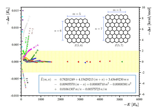
The second way to reduce the energy residuals further is to include the energies of some of these larger flakes in the fitting procedure. For the needs of the current analysis, we decided to include all 9 DFTB energies $E\left(m,n\right)$ of the larger flakes listed in Table 1 in the fitting set together with the previously used 121 DFTB energies $E\left(m,n\right)$ with $10\le m,n\le 20$. This new fitting set was used together with the $B=\{1,m+n,mn,m-n\}$ and $H=\{1,m+n,mn,m-n,m^2,n^2,m/n,n/m\}$ fitting functions sets; the resulting fitting protocols were abbreviated as $B^{\ast }$ and $H^{\ast }$, respectively. The list of the fitting coefficients for $B^{\ast }$ and $H^{\ast }$ is given in Table 2. The performance of these protocols is summarized in Figure 7; the left panel of this figure shows the residuals obtained with the $B^{\ast }$ protocol, and the right panel shows the residuals obtained with the $H^{\ast }$ protocol. For $B^{\ast }$, including the 9 energies of the larger flakes allowed us to reduce the energy residuals to less than $\pm 2$ kcal/mol. The performance of $H^{\ast }$ is particularly stunning: all the energies $E\left(m,n\right)$ with $10\le m,n$ are reproduced with practically vanishing residuals. Since all the previously used test points were included in the fitting set, to test the quality of these two new protocols, we decided to include two new large flakes, $Z\left(25,35\right)$ and $Z\left(40,35\right)$, in our analysis. (Note that for the 11 large rectangular flakes employed here for tests, the DFTB optimizations were performed less rigorously, with the force convergence criterion being, at most, $3\times {10}^{-5}$ a.u.) Figure 7 shows that both protocols perform well for these two new flakes, but the performance of $H^{\ast }$ is outstanding. We feel that it is worth explicitly stating the accurate energy expression $\tilde{E}(m,n)$ constructed using the protocol $H^{\ast }$,

$$\begin{array}{ccc}\hfill \tilde{E}(m,n)& =& 0.78201249+4.15429213\left(m+n\right)+3.43649230mn\hfill \\ & -& 0.00905570\left(m-n\right)+0.00000710m^2-0.00000381n^2\hfill \\ & +& 0.01061307m/n-0.00375723n/m\hfill \end{array}$$

(11)

5. Results and Discussion

Several interesting aspects of our work are worth highlighting:

 (i) 

Figure 6 and the left panel of Figure 7 clearly show that the accuracy of the constructed energy expression $\tilde{E}(m,n)$ deteriorates when one extrapolates it outside of the fitting set. A similar effect is also expected for the best-constructed energy expression $\tilde{E}(m,n)$ in Equation (11) when used for very large flakes with $m,n\ge 60$. However, as the current study shows, such a problem can be easily circumvented by adding a few new very large flakes $Z\left(m,n\right)$ with relevant values of m and n to the fitting set. For researchers interested in such extensions, we have included all the DFTB input files in the Supplementary Materials Section of this manuscript. The DFTB geometry optimization for the largest flake considered here, $Z\left(40,35\right)$ with the molecular formula C₂₉₅₀H₁₅₂, took approximately several weeks on a 100-core computer. The reader should be aware that the optimization of a larger flake might take a considerably longer time. An interesting alternative here could be a theoretical analysis of the contributions to the total energy from the finite edge effects and possibly quantifying such an influence using non-obvious, new $(m,n)$-dependent basis functions. Such a development is expected to improve the description of small flakes and to permit the extrapolation of the energy formula to really large values of m and n that presently escape the possibility of direct quantum chemical calculations.

 (ii) 

Small rectangular graphene flakes are known for their various interesting chemical deviations from the typical behavior of polycyclic hydrocarbons, including their open-shell ground state [53,54,55,56] and pronounced radical character [57,58,59,60,61,62,63]. Our work shows that larger flakes are more uniform, suggesting that the transition from finite, pyrene-like, small flakes to infinite, graphene-like, large flakes happens in the regime of $m,n\approx 10$. To investigate this issue in more detail, we have analyzed the distribution of the CC bond lengths and CCC bond angles in the transition from small to large flakes. Before discussing the results, let us only briefly comment that in the transition from small to large flakes, one would expect that the bond lengths and bond angles would become more uniform, approaching the values corresponding to an infinite graphene sheet, i.e., CC bond lengths of 1.42–1.43 Å obtained from the DFT calculations [64,65,66,67] and of 1.42 Å obtained from experiment and an angle of 120${}^{\circ }$ corresponding to a hexagonal geometry. The results for square flakes defined by the formula $Z\left(k,k\right)$ for $k=2$–20 are presented in Figure 8.

These results show that the convergence to the graphene-like values is fast. In principle, the flakes $Z\left(6,6\right)$ already show distributions similar to $Z\left(20,20\right)$. In addition to square-shaped flakes, it is interesting to check for similar convergence properties for rectangular flakes. In Figure 9, we show analogous distributions of CC bond lengths and CCC bond angles for two families of rectangular flakes, $Z\left(20,k\right)$ and $Z\left(k,20\right)$, with values of $k=2$–20. In both cases, the convergence toward the graphene-like regime is obtained faster than for the square flakes; this effect is particularly fast for the polyacene-like flakes $Z\left(20,k\right)$. Despite the fast convergence to the graphene-like regime, the finite edge effects are clearly visible in all the distributions, suggesting that the hydrogen termination and edge effects constitute important local perturbations.

 (iii) 

The parameters of the fit tabulated in Table 2 show surprisingly large inertias with respect to the extension of the function set with new variables. This behavior suggests that the energy decomposition has physical meaning, and its coefficients can be interpreted as sums of various energy contributions. For a flake $Z\left(m,n\right)$, the contributions can be easily identified:

• The energy ${ϵ}_{\mathrm{H}}$ of a hydrogen atom with multiplicity $2(m+n)+2$;
• The energy ${ϵ}_{\mathrm{C}}$ of a carbon atom with multiplicity $2mn+2(m+n)$;
• The energy ${ϵ}_{\mathrm{O}}$ of an aromatic ring with multiplicity $mn$;
• The energy ${ϵ}_{\mathrm{CC}}$ of a C–C bond with multiplicity $3mn+2(m+n)-1$;
• The energy ${ϵ}_{\mathrm{CH}}$ of a C–H bond with multiplicity $2(m+n)+2$.

Unfortunately, all these contributions involve only 3 fitting functions ($\{1,m+n,$ and $mn\}$), showing that a unique determination of the five parameters ${ϵ}_{\mathrm{H}}$, ${ϵ}_{\mathrm{C}}$, ${ϵ}_{\mathrm{O}}$, ${ϵ}_{\mathrm{CC}}$, and ${ϵ}_{\mathrm{CH}}$ from the three coefficients $c_1$, $c_2$, and $c_3$ is not possible from our analysis. In the future studies, we plan to extend our analysis to other structured graphene flakes, including prolate rectangles $Pr(k,m,n)$ [11,68], oblate rectangles $Ob(m,n)$ [11,69], and hexagons $O(k,m,n)$[11,46]. We expect that the distinct dependence of the total energy on the structural parameters for these structures will help to uniquely determine the five parameters ${ϵ}_{\mathrm{H}}$, ${ϵ}_{\mathrm{C}}$, ${ϵ}_{\mathrm{O}}$, ${ϵ}_{\mathrm{CC}}$, and ${ϵ}_{\mathrm{CH}}$ defined above.

 (iv) 

The energies used to construct the energy expression given by Equation (11) in addition to the usual size and shape dependence encoded by the parameters m and n also include contributions related to the geometry relaxation effects. In our study, all these components are treated collectively. It would be very interesting to consider the relaxation effects individually, for example, by starting the geometry optimization from a rectangular patch of an idealized infinite graphene sheet with uniform hydrogen terminations. The relaxation effects can be divided into three types of contributions: (1) those corresponding to the relaxation of the carbon sublattice, (2) those corresponding to the relaxation of the hydrogen sublattice, and (3) those corresponding to the synergic relaxation of both lattices simultaneously. Such an analysis is beyond the scope of the current study.

 (v) 

Numerous studies tried to correlate various topological invariants with the energetic stability of polycyclic aromatic hydrocarbons. The vast efforts of the graph-theoretically oriented chemists over the last few decades have created substantial literature on this topic. (Probably the best existing account describing the body of results on the Kekulé count $\mathcal{K}$ is the monography of Cyvin and Gutman [11]; the results on other invariants are scattered throughout the literature.) Our study may show that such an effort might be somewhat superfluous as similar effects can be achieved more readily by correlating the energetics with appropriate structural parameters (and their simple algebraic functions) of the whole family of analyzed structures.

6. Conclusions

We have computed the DFTB energies $E\left(m,n\right)$ of rectangular graphene flakes $Z\left(m,n\right)$ with $1\le m,n\le 20$ at their optimized geometries. The resulting set of energies has been used to construct an approximate energy expression $\tilde{E}(m,n)$ for $E\left(m,n\right)$ in a form of a linear combination of various simple functions of the structural parameters m and n. In order to construct an accurate energy expression $\tilde{E}(m,n)$, several important factors have been explicitly considered in our work:

 (i) 

It has been recognized that small graphene flakes $Z\left(m,n\right)$ with $1\le m,n\le 9$ are structurally dissimilar to larger flakes due to their finite-size effects. Those structures have been excluded from the fitting set, which finally comprised 121 energies of flakes $Z\left(m,n\right)$ with $10\le m,n\le 20$.

 (ii) 

It has been noted that in order to be able to extrapolate the energy expression $\tilde{E}(m,n)$ outside of the fitting region, we need to include in the fitting set several larger structures $Z\left(m,n\right)$ with $20\le m,n$.

 (iii) 

The set of fitting functions resulting from structural considerations and comprising physically meaningful variables $\{1,m+n,mn,m-n\}$ needs to be expanded to $\{1,m+n,mn,m-n,m^2,n^2,n/m,m/n\}$. The physical interpretation of these new variables remains to be understood.

 (iv) 

Performance tests of the energy expression $\tilde{E}(m,n)$ have been performed using two additional graphene flakes, $Z\left(25,35\right)$ and $Z\left(40,35\right)$.

The best approximation to $E\left(m,n\right)$ was produced using a fitting protocol abbreviated as $H^{\ast }$ (for details, see Table 2); the explicit form of the resulting $\tilde{E}(m,n)$ is given by Equation (11). This expression is very accurate and falls withing the requirement of chemical accuracy (i.e., the energy residuals $\Delta ϵ(m,n)$ are smaller than $\pm 2$ kcal/mol) for all graphene flakes $Z\left(m,n\right)$ with $10\le m,n\le 20$ used in the current study; in fact, all the relevant residuals are almost negligible (for details, see the right panel of Figure 7).

References

- Cramer, C.J. Essentials of Computational Chemistry: Theories and Models, 1st ed.; Wiley: Hoboken, NJ, USA, 2004. [Google Scholar]
- Elstner, M.; Seifert, G. Density functional tight binding. Philos. Trans. R. Soc. 2014, 372, 20120483. [Google Scholar] [CrossRef] [PubMed]
- Keith, J.A.; Vassilev-Galindo, V.; Cheng, B.; Chmiela, S.; Gastegger, M.; Müller, K.R.; Tkatchenko, A. Combining machine learning and computational chemistry for predictive insights into chemical systems. Chem. Rev. 2021, 121, 9816–9872. [Google Scholar] [CrossRef] [PubMed]
- Rupp, M.; Tkatchenko, A.; Müller, K.R.; von Lilienfeld, O.A. Fast and accurate modeling of molecular atomization energies with machine learning. Phys. Rev. Lett. 2012, 108, 058301. [Google Scholar] [CrossRef]
- Montavon, G.; Rupp, M.; Gobre, V.; Vazquez-Mayagoitia, A.; Hansen, K.; Tkatchenko, A.; Müller, K.R.; von Lilienfeld, O.A. Machine learning of molecular electronic properties in chemical compound space. New J. Phys. 2013, 15, 095003. [Google Scholar] [CrossRef]
- Schütt, K.T.; Arbabzadah, F.; Chmiela, S.; Müller, K.R.; Tkatchenko, A. Quantum-chemical insights from deep tensor neural networks. Nat. Commun. 2017, 8, 13890. [Google Scholar] [CrossRef]
- De, S.; Bartók, A.P.; Csányi, G.; Ceriotti, M. Comparing molecules and solids across structural and alchemical space. Phys. Chem. Chem. Phys. 2016, 18, 13754–13769. [Google Scholar] [CrossRef] [PubMed]
- Chmiela, S.; Tkatchenko, A.; Sauceda, H.E.; Poltavsky, I.; Schütt, K.T.; Müller, K.R. Machine learning of accurate energy-conserving molecular force fields. Sci. Adv. 2017, 3, e1603015. [Google Scholar] [CrossRef]
- Faber, F.A.; Hutchison, L.; Huang, B.; Gilmer, J.; Schoenholz, S.S.; Dahl, G.E.; Vinyals, O.; Kearnes, S.; Riley, P.F.; von Lilienfeld, O.A. Prediction errors of molecular machine learning models lower than hybrid DFT error. J. Chem. Theory Comput. 2017, 13, 5255–5264. [Google Scholar] [CrossRef] [PubMed]
- Schütt, K.T.; Sauceda, H.E.; Kindermans, P.J.; Tkatchenko, A.; Müller, K.R. SchNet—A deep learning architecture for molecules and Materials. J. Chem. Phys. 2018, 148, 241722. [Google Scholar] [CrossRef]
- Cyvin, S.J.; Gutman, I. Kekulé Structures in Benzenoid Hydrocarbons; Springer: Berlin/Heidelberg, Germany, 1988. [Google Scholar]
- Gutman, I.; Cyvin, S.J.; si Chen, R.; rong Lin, K. Number of Kekulé structures of multiple zigzag chain aromatics. Monatsh. Chem. 1993, 124, 117–125. [Google Scholar] [CrossRef]
- Weiße, A.; Fehske, H. Exact diagonalization techniques. In Computational Many-Particle Physics; Fehske, H., Schneider, R., Weiße, A., Eds.; Springer: Berlin/Heidelberg, Germany, 2008; pp. 529–544. [Google Scholar]
- James, D.K.; Tour, J.M. Graphene: Powder, flakes, ribbons, and sheets. Acc. Chem. Res. 2013, 46, 2307–2318. [Google Scholar] [CrossRef] [PubMed]
- Kairi, M.I.; Dayou, S.; Kairi, N.I.; Bakar, S.A.; Vigolo, B.; Mohamed, A.R. Toward high production of graphene flakes—A review on recent developments in their synthesis methods and scalability. J. Mater. Chem. A 2018, 6, 15010–15026. [Google Scholar] [CrossRef]
- Rathinavel, S.; Priyadharshini, K.; Panda, D. A review on carbon nanotube: An overview of synthesis, properties, functionalization, characterization, and the application. Mater. Sci. Eng. B 2021, 268, 115095. [Google Scholar] [CrossRef]
- Fowler, P.W.; Manolopoulos, D.E. An Atlas of Fullerenes; Dover: Mineola, NY, USA, 2006. [Google Scholar]
- Schwerdtfeger, P.; Wirz, L.; Avery, J. Program Fullerene: A software package for constructing and analyzing structures of regular fullerenes. J. Comput. Chem. 2013, 34, 1508–1526. [Google Scholar] [CrossRef]
- Assadollahzadeh, B.; Schwerdtfeger, P. A systematic search for minimum structures of small gold clusters Aun(n=2–20) and their electronic properties. J. Chem. Phys. 2009, 131, 064306. [Google Scholar] [CrossRef] [PubMed]
- Assadollahzadeh, B.; Schäfer, S.; Schwerdtfeger, P. Electronic properties for small tin clusters Snn(n≤20) from density functional theory and the convergence toward the solid state. J. Comput. Chem. 2010, 31, 929–937. [Google Scholar] [CrossRef]
- Assadollahzadeh, B.; Thierfelder, C.; Schwerdtfeger, P. From clusters to the solid state: Global minimum structures for cesium clusters Csn(n=2–20,∞) and their electronic properties. Phys. Rev. B 2008, 78, 245423. [Google Scholar] [CrossRef]
- Firouzi, R.; Zahedi, M. Polyacenes electronic properties and their dependence on molecular size. J. Mol. Struct. Theochem 2008, 862, 7–15. [Google Scholar] [CrossRef]
- Li, W.; Irle, S.; Witek, H.A. Convergence in the evolution of nanodiamond Raman spectra with particle size: A theoretical investigation. ACS Nano 2010, 4, 4475–4486. [Google Scholar] [CrossRef]
- Medintz, I.L.; Uyeda, H.T.; Goldman, E.R.; Mattoussi, H. Quantum dot bioconjugates for imaging, labelling and sensing. Nat. Mater. 2005, 4, 435–446. [Google Scholar] [CrossRef]
- Resch-Genger, U.; Grabolle, M.; Cavaliere-Jaricot, S.; Nitschke, R.; Nann, T. Quantum dots versus organic dyes as fluorescent labels. Nat. Methods 2008, 5, 763–775. [Google Scholar] [CrossRef] [PubMed]
- Walkey, C.; Sykes, E.A.; Chan, W.C.W. Application of semiconductor and metal nanostructures in biology and medicine. Hematology 2009, 2009, 701–707. [Google Scholar] [CrossRef]
- Zadeh, D.H. Atomic excited states and the related energy levels. J. Mol. Model. 2022, 28, 282. [Google Scholar] [CrossRef]
- Caramori, G.F.; Østrøm, I.; Ortolan, A.O.; Nagurniak, G.R.; Besen, V.M.; noz Castro, A.M.; Orenha, R.P.; Parreira, R.L.T.; Galembeck, S.E. The usefulness of energy decomposition schemes to rationalize host–guest interactions. Dalton Trans. 2020, 49, 17457–17471. [Google Scholar] [CrossRef]
- Mitoraj, M.P.; Michalak, A.; Ziegler, T. A combined charge and energy decomposition scheme for bond analysis. J. Chem. Theory Comput. 2009, 5, 962–975. [Google Scholar] [CrossRef] [PubMed]
- Gimferrer, M.; Danés, S.; Andrada, D.M.; Salvador, P. Merging the energy decomposition analysis with the interacting quantum atoms approach. J. Chem. Theory Comput. 2023, 19, 3469–3485. [Google Scholar] [CrossRef] [PubMed]
- Mutsuji, A.; Saita, K.; Maeda, S. An energy decomposition and extrapolation scheme for evaluating electron transfer rate constants: A case study on electron self-exchange reactions of transition metal complexes. RSC Adv. 2023, 13, 32097–32103. [Google Scholar] [CrossRef] [PubMed]
- Francisco, E.; Pendás, A.M.; Blanco, M.A. A molecular energy decomposition scheme for atoms in molecules. J. Chem. Theory Comput. 2006, 1, 90–102. [Google Scholar] [CrossRef]
- Gutman, I.; Gojak, S.; Furtula, B.; Radenković, S.; Vodopivec, A. Relating total π-electron energy and resonance energy of benzenoid molecules with Kekulé- and Clar-structure-based parameters. Monatsh. Chem. 2006, 137, 1127–1138. [Google Scholar] [CrossRef]
- Gojak, S.; Gutman, I.; Radenković, S.; Vodopivec, A. Relating resonance energy with the Zhang-Zhang polynomial. J. Serb. Chem. Soc. 2007, 72, 665–671. [Google Scholar] [CrossRef]
- Kekulé, A. Sur la constitution des substances aromatiques. Bull. Soc. Chim. Fr. 1865, 2, 98–110. [Google Scholar]
- Clar, E. The aromatic sextet. In Mobile Source Emissions Including Policyclic Organic Species; Rondia, D., Cooke, M., Haroz, R.K., Eds.; Springer: Dordrecht, The Netherlands, 1983; pp. 49–58. [Google Scholar] [CrossRef]
- Zhang, F.; Zhang, H. A new enumeration method for Kekulé structures of hexagonal systems with forcing edges. J. Mol. Struct. Theochem 1995, 331, 255–260. [Google Scholar] [CrossRef]
- Zhang, H.P.; Zhang, F.J. The Clar covering polynomial of hexagonal systems I. Discret. Appl. Math. 1996, 69, 147–167. [Google Scholar] [CrossRef]
- Gutman, I.; Furtula, B.; Balaban, A.T. Algorithm for simultaneous calculations of Kekulé and Clar structure counts, and Clar number of benzenoid molecules. Polycycl. Aromat. Compd. 2006, 26, 17–35. [Google Scholar] [CrossRef]
- Chou, C.P.; Witek, H.A. An algorithm and FORTRAN program for automatic computation of the Zhang-Zhang polynomial of benzenoids. MATCH Commun. Math. Comput. Chem. 2012, 68, 3–30. [Google Scholar]
- Chou, C.P.; Witek, H.A. ZZDecomposer: A graphical toolkit for analyzing the Zhang-Zhang polynomials of benzenoid structures. MATCH Commun. Math. Comput. Chem. 2014, 71, 741–764. [Google Scholar]
- Žigert Pleteršek, P. Equivalence of the generalized Zhang-Zhang polynomial and the generalized cube polynomial. MATCH Commun. Math. Comput. Chem. 2018, 80, 215–226. [Google Scholar]
- Furtula, B.; Radenković, S.; Redžepović, I.; Tratnik, N.; Žigert Pleteršek, P. The generalized Zhang–Zhang polynomial of benzenoid systems – theory and applications. Appl. Math. Comput. 2022, 418, 126822. [Google Scholar] [CrossRef]
- Gutman, I.; Borovićanin, B. Zhang-Zhang polynomial of multiple linear hexagonal chains. Z. Naturforsch. A 2006, 61, 73–77. [Google Scholar] [CrossRef]
- Chou, C.P.; Kang, J.S.; Witek, H.A. Closed-form formulas for the Zhang–Zhang polynomials of benzenoid structures: Prolate rectangles and their generalizations. Discret. Appl. Math. 2016, 198, 101–108. [Google Scholar] [CrossRef]
- Witek, H.A.; Podeszwa, R.; Langner, J. Closed–form formulas for Zhang–Zhang polynomials of hexagonal graphene flakes O(k,m,n) with k,m=1--7 and arbitrary n. MATCH Commun. Math. Comput. Chem. 2021, 83, 165–194. [Google Scholar]
- Witek, H.A. Zhang–Zhang polynomials of multiple zigzag chains revisited: A connection with the John–Sachs theorem. Molecules 2021, 26, 2524. [Google Scholar] [CrossRef]
- Gaus, M.; Cui, Q.; Elstner, M. DFTB3: Extension of the self-consistent-charge density-functional tight-binding method (SCC-DFTB). J. Chem. Theory Comput. 2011, 7, 931–948. [Google Scholar] [CrossRef]
- Gaus, M.; Goez, A.; Elstner, M. Parametrization and benchmark of DFTB3 for organic molecules. J. Chem. Theory Comput. 2013, 9, 338–354. [Google Scholar] [CrossRef]
- Hourahine, B.; Aradi, B.; Blum, V.; Bonafé, F.; Buccheri, A.; Camacho, C.; Cevallos, C.; Deshaye, M.Y.; Dumitrică, T.; Dominguez, A.; et al. DFTB+, a software package for efficient approximate density functional theory based atomistic simulations. J. Chem. Phys. 2020, 152, 124101. [Google Scholar] [CrossRef] [PubMed]
- Trefethen, L.N.; Bau, D., III. Numerical Linear Algebra; SIAM: Philadelphia, PA, USA, 1997. [Google Scholar]
- Press, W.H.; Teukolsky, S.A.; Vetterling, W.T.; Flannery, B.P. Numerical Recipes in Fortran 77: The Art of Scientific Computing, 2nd ed.; Cambridge University Press: Cambridge, UK, 1992. [Google Scholar]
- Houk, K.N.; Lee, P.S.; Nendel, M. Polyacene and cyclacene geometries and electronic structures: Bond equalization, vanishing band gaps, and triplet ground states contrast with polyacetylene. J. Org. Chem. 2001, 66, 5517–5521. [Google Scholar] [CrossRef]
- Bendikov, M.; Duong, H.M.; Starkey, K.; Houk, K.N.; Carter, E.A.; Wudl, F. Oligoacenes: Theoretical prediction of open-shell singlet diradical ground states. J. Am. Chem. Soc. 2004, 126, 7416–7417. [Google Scholar] [CrossRef]
- Jiang, D.; Dai, S. Electronic ground state of higher acenes. J. Phys. Chem. A 2008, 112, 332–335. [Google Scholar] [CrossRef]
- Qu, Z.; Zhang, D.; Liu, C.; Jiang, Y. Open-shell ground state of polyacenes: A valence bond study. J. Phys. Chem. A 2009, 113, 7909–7914. [Google Scholar] [CrossRef] [PubMed]
- Lee, J.; Small, D.W.; Epifanovsky, E.; Head-Gordon, M. Coupled-cluster valence-bond singles and doubles for strongly correlated systems: Block-tensor based implementation and application to oligoacenes. J. Chem. Theory Comput. 2017, 13, 602–615. [Google Scholar] [CrossRef]
- Das, A.; Müller, T.; Plasser, F.; Lischka, H. Polyradical character of triangular non-Kekulé structures, zethrenes, p-quinodimethane-linked bisphenalenyl, and the Clar goblet in comparison: An extended multireference study. J. Phys. Chem. A 2016, 120, 1625–1636. [Google Scholar] [CrossRef] [PubMed]
- Yeh, C.N.; Chai, J.D. Role of Kekulé and non-Kekulé structures in the radical character of alternant polycyclic aromatic hydrocarbons: A TAO-DFT study. Sci. Rep. 2016, 6, 30562. [Google Scholar] [CrossRef] [PubMed]
- Plasser, F.; Pašalić, H.; Gerzabek, M.H.; Libisch, F.; Reiter, R.; Burgdörfer, J.; Müller, T.; Shepard, R.; Lischka, H. The multiradical character of one- and two-dimensional graphene nanoribbons. Angew. Chem. Int. Ed. 2013, 52, 2581–2584. [Google Scholar] [CrossRef] [PubMed]
- Urgel, J.I.; Mishra, S.; Hayashi, H.; Wilhelm, J.; Pignedoli, C.A.; Giovannantonio, M.D.; Widmer, R.; Yamashita, M.; Hieda, N.; Ruffieux, P.; et al. On-surface light-induced generation of higher acenes and elucidation of their open-shell character. Nat. Commun. 2019, 10, 1–9. [Google Scholar] [CrossRef]
- Trinquier, G.; David, G.; Malrieu, J.P. Qualitative views on the polyradical character of long acenes. J. Phys. Chem. A 2018, 122, 6926–6933. [Google Scholar] [CrossRef]
- Minkin, V.I.; Starikov, A.G.; Starikova, A.A. Acene-linked zethrenes and bisphenalenyls: A DFT search for organic tetraradicals. J. Phys. Chem. A 2021, 125, 6562–6570. [Google Scholar] [CrossRef]
- Yang, J.; Yuan, Y.; Chen, G. First–principles study of potassium adsorption and diffusion on graphene. Mol. Phys. 2019, 118, e1581291. [Google Scholar] [CrossRef]
- Koh, Y.; Manzhos, S. Curvature drastically changes diffusion properties of Li and Na on graphene. MRS Commun. 2013, 3, 171–175. [Google Scholar] [CrossRef]
- Flores, M.Z.S.; Autreto, P.A.S.; Legoas, S.B.; Galvao, D.S. Graphene to graphane: A theoretical study. Nanotechnology 2009, 20, 465704. [Google Scholar] [CrossRef] [PubMed]
- Malyi, O.I.; Sopiha, K.; Kulish, V.V.; Tan, T.L.; Manzhos, S.; Persson, C. A computational study of Na behavior on graphene. Appl. Surf. Sci. 2015, 333, 235–243. [Google Scholar] [CrossRef]
- Yen, T.F. Resonance topology of polynuclear aromatic hydrocarbons. Theor. Chim. Acta 1971, 20, 399–404. [Google Scholar] [CrossRef]
- Gutman, I. Topological properties of benzenoid systems. XXVIII. Number of Kekulé structures of some benzenoid hydrocarbons. MATCH Commun. Math. Comput. Chem. 1985, 17, 3–10. [Google Scholar]
- He, B.H.; Langner, J.; Witek, H.A. Hexagonal flakes as fused parallelograms: A determinantal formula for Zhang-Zhang polynomials of the O(2,m,n) benzenoids. J. Chin. Chem. Soc. 2021, 68, 1231–1242. [Google Scholar] [CrossRef]
- He, B.H.; Langner, J.; Podeszwa, R.; Witek, H.A. Can the John–Sachs theorem be extended to Clar covers? MATCH Commun. Math. Comput. Chem. 2021, 83, 141–163. [Google Scholar]
- Langner, J.; Witek, H.A. Interface theory of benzenoids. MATCH Commun. Math. Comput. Chem. 2020, 84, 143–176. [Google Scholar]
- Langner, J.; Witek, H.A. Interface theory of benzenoids: Basic applications. MATCH Commun. Math. Comput. Chem. 2020, 84, 177–215. [Google Scholar]
- Langner, J.; Witek, H.A. ZZ polynomials of regular m-tier benzenoid strips as extended strict order polynomials of associated posets. Part 1. Proof of equivalence. MATCH Commun. Math. Comput. Chem. 2022, 87, 585–620. [Google Scholar] [CrossRef]
Figure 1.
Two examples of multiple zigzag chains . The index m represents the length of the zigzag edge of these rectangular flakes, while the index n corresponds to the length of the armchair edge. The shape and the symmetry of the flake are slightly different for even and odd values of n.
Figure 2.
The energies of the optimized graphene flakes can be arranged in the shape of a trapezoid, in which the vertical lines correspond to constant values of m and the diagonal lines correspond to a constant values of n.
Figure 3.
Energy residual corresponding to the fit obtained with a set . Points depicted in identical colors have identical values of m, and points depicted with identical symbols have identical values of n. For the convenience of the reader, the energy residuum scale is given in hartree (left axis) and in kcal/mol (right axis).
Figure 4.
Energy residuals corresponding to the fit obtained with a set . Points depicted in identical colors have identical values of m, and points depicted with identical symbols have identical values of n. For the convenience of the reader, the energy residuum scale is given in hartree (left axis) and in kcal/mol (right axis).
Figure 5.
Further improvement of energy residuals obtained using the fitting set and (left) and (right). For the meaning of M and N, see text. The yellow background depicts region of kcal/mol corresponding to chemical accuracy.
Figure 6.
(Left): The residuals for the 9 new larger flakes with , marked here with red triangles, show a rather large systematic departure from the chemical accuracy limit and suggest that the energy expression constructed using the fitting function set and 121 DFTB energy values of smaller flakes with cannot be easily extrapolated to larger structures. (Right): Various means to solve this problem are discussed in text. Here, we show that extending the fitting function set to can substantially reduce the residuals for these 9 new larger flakes, making all of them smaller than kcal/mol. The yellow background depicts region of kcal/mol corresponding to chemical accuracy.
Figure 7.
Further improvement of energy residuals obtained using the set (left panel) and (right panel). The star signifies that 121 DFTB energies with are used for the fitting process along with the 9 additional DFTB energies of the flakes listed in Table 1. The residuals for the additional points are marked with red triangles. Two new flakes, (with a residue marked with a blue triangle) and (with a residue marked with a green triangle), are used to assess the quality of the constructed energy expressions . The yellow background depicts region of kcal/mol corresponding to chemical accuracy.
Figure 8.
Distributions of the CC bond lengths (left) and CCC bond angles (right) in square flakes suggest that the graphene regime is already achieved for quite small flakes.
Figure 9.
Distributions of the CC bond lengths (left panels) and CCC bond angles (right panels) in rectangular flakes (upper panels) and (lower panels) suggest that the transition to graphene-like regime is achieved faster than for square flakes.