Magnetostrictive and Magnetoactive Effects in Piezoelectric Polymer Composites

Abstract

A mesoscopic model for a polymer-based magnetoelectric (ME) composite film is developed. The film is assumed to consist of a piezoelectric polymer matrix of the PVDF type filled with CFO-like single-domain nanoparticles. The model is treated numerically and enables one to obtain in detail the intrinsic distributions of mechanical stress, polarization and electric potential and helps to understand the influence of the main configurational parameters, viz., the poling direction and the orientational order of the particle magnetic anisotropy axes on the electric response of the film. As the model is fairly simple—it uses the RVE-like (Representative Volume Element) approach with a single-particle cell—the results obtained are rather of qualitative than quantitative nature. However, the general conclusions seem to be independent of the particularities of the model. Namely, the presented results establish that the customary ME effect in composite films always comprises at least two contributions of different origins, viz., the magnetostrictive and the magnetoactive (magnetorotational) ones. The relative proportion between those contributions is quite movable depending on the striction coefficient of the particles and the stiffness of the polymer matrix. This points out the necessity to explicitly take into account the magnetoactive contribution when modeling the ME response of composite films and when interpreting the measurements on those objects.

1. Introduction

The essence of the functionality of magnetoelectric (ME) composites is the mediating role of mechanical stresses. Along this route either the magnetic phase acts on the piezoelectric one (the direct ME effect) or vice versa (the inverse ME effect). From that stem all the versatile applications of ME transducers and convertors as sensors and actuators [1,2], non-volatile memory [3], energy harvesters [4,5,6], activators of tissue regeneration processes [7,8,9,10,11], etc.

1.1. Magnetostrictive Composites

In the conventional paradigm, the mechanical link in the ME transformation is established by the magnetostriction effect, i.e., the change of dimensions of a ferromagnetic object under magnetization. This equally relates to solid two-component systems like ferromagnet (FM)+piezoelectric (PE) and to two- and three-component polymeric compositions of the FM+polymeric PE or FM+PE polymer+solid PE types. Therefore, to make the conversion efficient, the magnetic powders of the substances with high magnetostriction coefficients are used, first place, cobalt ferrite Co ${}_{1-x}$Fe${}_{2+x}$O${}_4$ (CFO) and Terfenol-D.

Typical solid PE materials used in the ME composites are ceramics BaTiO${}_3$ (BTO) and Pb[Zr${}_x$Ti${}_{1-x}$]O${}_3$ (PZT). The most popular polymeric piezoelectrics are PVDF (poly-vinylidene fluoride) and its co-polymers. A substantial part of their supramolecular structure consists of the crystallite $\beta$ phase that displays high piezoelectric response comparable to that of customary solid piezoelectrics [12,13,14]. To align the electric polarization directions in the $\beta$-phase domains, the PVDF films are subjected to the poling procedure and are worked on with a high-strength electric field.

When producing PVDF-based composite films, CFO nanoparticles are added to the yet non-solidified polymer, then the mixture is stirred up to homogenize and finally dried, see [15,16,17,18], for example. The working conditions for such magnetostrictive films are set with the aid of a constant magnetic (bias) field ${\mathit{H}}_0$. Under the action of ${\mathit{H}}_0$, the ferrite particles change their shapes and become the sites of local (mesoscopic) mechanical stresses. Those stresses either directly act on the surrounding PE phase (a two-component composite) or perturb the polymeric matrix that, in turn, transfers the stress to the embedded PE particles (a three-component composite).

In any case, the applied field ${\mathit{H}}_0$ induces a stationary electric polarization that manifests itself as the transverse voltage difference $\mathsf{\Delta }\phi$ between the film faces. This state is used as the operating point of an ME device, the bias strength is chosen in such a way that the steepness of function $d\lambda /d{H}_0$ was maximal; here $\lambda$ is the coefficient of linear magnetostriction that characterizes the field-induced FM particle strain. Such a composite responds to an applied probing field ${\mathit{H}}_t$ by generating an electric signal: the voltage difference at the film changes by increment $\delta \phi$. In general, the magnitude of $\delta \phi$ depends nonlinearly on the bias field as the magnetostriction is saturated under a strong field. However, for $H_t\ll H_0$ the electric response is linear in $H_t$. Because of that, the efficiency of ME conversion is conventionally expressed in terms of coefficient ${\alpha }_V=\delta \phi /(\mathsf{\ell }·H_t)$ which is a specific ME ‘susceptibility’ of the film; here ℓ is the film thickness.

1.2. Magnetoactive Composites

A particle of a magnetically-hard ferrite (CFO, for example) possesses a permanent magnetic moment $\mathit{\mu }$ of its own, and due to that any field $\mathit{H}$ that is non-collinear with $\mathit{\mu }$ creates a torque which, having been transferred to the particle anisotropy axis, strives to turn the particle body in such a way that $\mathit{\mu }$ aligns with $\mathit{H}$. In such a situation, a particle that dwells inside a composite produces mechanical stresses in its surroundings. These stresses, however, have nothing to do with the magnetostriction effect as the particle shape does not change. Let us term this way of generating internal stresses as magnetoactive using the analogy with the magnetoactive polymers.

Therefore, in a magnetoactive composite, the origin of the electric signal is the same as in the magnetostrictive one, but the origin of the stress is different. As we have shown [19], the ME effect in a three-component magnetoactive composite but weakly depends on the elastic modulus of the matrix, so the latter might be varied in a wide range. On the other hand, the properties of three-component composites strongly depend on the mutual positions of the FM and PE particles. This structural “hypersensitivity” is absent in a two-component system of the FM/PVDF kind, and because of that, such systems are more appropriate for making magnetoactive composites.

Looking into the literature, one finds but few examples of the systems which might be considered magnetoactive or the prototypes of those. The more interesting is the case reported in Ref. [20] where the ME effect was studied in a dispersion of feroxyhyte $\delta$-Fe${}^{3+}$O(OH) nanosheets in PVDF-TrFE. Although feroxyhyte, being a ferrohydroxide, is but weakly magnetic, it is remarkable by the virtual absence of magnetostriction. Therefore, in the composite under study, the conventional ME mechanism was totally “switched-off”. As the magnetoelectric effect in this system was observed and measured, this means that in Ref. [20] the existence of the magnetoactive way of ME conversion has been demonstrated experimentally. A short discussion of that notable work and the essence of the effect discovered there might be found in Ref. [19].

Carrying on this line of considerations, one would suppose that the magnetoactive mechanism, in fact, should have rather significantly contributed (certainly, together with the magnetostrictive one) to the ME effect in the PVDF films filled with other anisometric objects: nanoplatelets of barium ferrite [21,22], metal hydroxide Co(II)Fe(III)-O(OH) [23], and metal nanowires [24].

2. Coexistence of the Magnetostrictive and Magnetoactive ME Effects

It follows that in any ME composite both effects—the magnetostrictive as well as the magnetoactive one—should coexist. Meanwhile, in the literature on composite polymer magnetoelectrics, both on research and on the technology of those materials, the focus of attention is exclusively set on the magnetostriction mechanism, see the reviews [5,25,26,27,28,29,30], for example. This is no surprise as those contributions are rather difficult to distinguish from one another in the measurement results.

The goal of the present work is to carry out, by means of numerical modeling, a comparative analysis of the above-described effects. For that, the following model system is used. A composite film consists of a polymer matrix with the properties of PVDF that is filled with fine spherical particles with the properties of CFO. The polar nature of the PVDF molecules ensures their strong adhesion to the particles, so that the latter may be treated as tightly “glued” to the matrix. Due to that, any shape or position changes of the particles induce stresses in the matrix (note that the accompanying deformations might be quite small) and by that create piezoelectric polarization. The matrix is assumed to have passed the poling procedure and, hence, is characterized by a “global” unit vector $\mathit{\nu }$ of piezoelectric anisotropy. The FM nanoparticles are single-domain but sufficiently large to be free of superparamagnetism. Given that, for their description, one may employ the Stoner–Wohlfarth model with uniaxial magnetic anisotropy of the easy-axis type whose direction is described by unit vector $\mathit{n}$.

Under the application of magnetic field $\mathit{H}$ that is non-collinear with $\mathit{n}$, the particle changes its shape, and by that induces the magnetostrictive part of the mechanical stress. Simultaneously, the magnetoactive part turns up as well. Indeed, at $\mathit{H}=0$ the particle magnetic moment $\mathit{\mu }$ points along one of the directions of the anisotropy axis: $\mathit{\mu }\Vert \mathit{n}$. As a single-domain particle is magnetized to saturation, its magnetic susceptibility along $\mathit{n}$ is zero; this implies that the susceptibility tensor of the particle may be presented in the form

$${\chi }_{ik}=\chi \left({\delta }_{ik}-n_i{n}_k\right).$$

(1)

In the field $\mathit{H}$ whose strength is below the lowest coercive force $K/M_s$ of the Stoner–Wohlfarth particle—here K is the anisotropy constant and $M_s$ saturation magnetization of the ferrite—the particle would magnetize according to

$$M_i=M_s{n}_i+{\chi }_{ik}{H}_k=M_s\left[n_i+\frac{H_k}{H_A}\left({\delta }_{ik}-n_i{n}_k\right)\right],$$

(2)

where $H_A=2K/M_s$ is the reference value of the anisotropy field. The torque that the particle exerts on the matrix is

$$\left(\mathit{\mu }\times \mathit{H}\right)=M_{s}Hv\left(\mathit{n}\times \mathit{h}\right)\left[1-\frac{H}{H_A}\left(\mathit{n}\mathit{h}\right)\right];$$

(3)

here $\mathit{\mu }=\mathit{M}v$ is the magnetic moment of a single-domain particle, v is its volume, $\mathit{h}=\mathit{H}/H$ is the unit vector of the field. Note that expressions (2) and (3) are valid to the first order in parameter $H/H_A$, that is, our consideration applies to the field range $H<\frac{1}{2}{H}_A=K/M_s$.

3. Superposition of the Effects: Qualitative View

To obtain a qualitative notion of how the magnetostrictive and magnetoactive (magnetorotational) mechanisms manifest themselves in joint action, we consider a 2D particle sitting inside a square cell filled with an elastic continuum; one of the cell sides is made immovable. In Figure 1 shear stress distributions for two variants of mutual orientations of the particle magnetic moment $\mathit{\mu }$ and applied field ${\mathit{H}}_0$ evaluated according to the procedure described in Section 5 are shown. The performed calculation employed the set of material parameters typical for the system CFO/PVDF; however, for the sake of visualization, the obtained values of strain are magnified by several orders. This modification reveals that magnetostriction deforms the particle: being initially a sphere it becomes prolate. Note, that in both panels, the acquired shapes of the particle are the same; this is because the magnetostriction effect does not depend on the absolute position of vectors $\mathit{n}$ and ${\mathit{H}}_0$ in the plane passing through them. On the other hand, the magnetorotational effect preserves the particle shape; it just strives to align the magnetic moment, together with the anisotropy axis, with the field direction. Unlike the previous one, in this response mode, the sign of the effect inverts depending on the relative orientation of vectors $\mathit{\mu }$ and ${\mathit{H}}_0$. From that one concludes that, given the positions of the reference vectors, the two above-mentioned effects may either counteract one another (Figure 1a) or act synergistically (Figure 1b).

4. Energy Functional of the Composite Film

The model object under consideration is a film made of a composite of the PVDF/CFO type. The film is constructed as an infinite layer of elementary representative cells rigidly fixed on a solid plane. The representative cell—two variants are shown in Figure 2—is a cube of edge ℓ at the center of which there is positioned a spherical magnetically hard particle of radius $R_p$ the direction of whose magnetic anisotropy easy axis is defined by the unit vector $\mathit{n}$. The rest of the cell is filled with a PVDF-like polymer that had been subjected to poling that imparted to it a piezoelectric anisotropy characterized by the unit vector $\mathit{\nu }$; the lower ($z=0$) face of the cell is immovable. Inside the layer, the cells are coupled by means of periodic boundary conditions imposed on all the basic thermodynamic variables, viz., mechanical stresses and strains and magnetic and electric fields. All the layer is embedded in the computational box whose dimensions in the $Oz$ direction are far greater than the film thickness. In this scheme, the average variables evaluated for a single cell coincide with those of the whole layer.

The 3D problem of evaluating the state of the representative cell is formulated in terms of the finite-strain theory. In that approach, the deformation of a body is described as its transition from the initial state to an actual one. Accordingly, a point whose position in the initial state was given by radius-vector $\mathit{r}$, in the actual state, i.e., after deformation, is positioned at $\mathit{R}=\mathit{r}+\mathit{u}$, where $\mathit{u}$ is the displacement vector. In this framework, the role of the spatial derivative is allotted to the deformation gradient $\mathbf{F}=\mathbf{I}+{(\nabla \mathit{u})}^{\mathrm{T}}$ whereas the strain tensor is defined as $\mathbf{E}=\frac{1}{2}\left({\mathbf{F}}^{\mathrm{T}}·\mathbf{F}-\mathbf{I}\right)$ where $\mathbf{I}$ is the unit tensor. Further details are given in Appendix A below.

For the modeling, the representative cell in the initial state is presented as a sum of spatial regions: ${\Omega }_{\mathrm{m}}^{\left(0\right)}$ and ${\Omega }_{\mathrm{p}}^{\left(0\right)}$ occupied by the FM particle and the polymer matrix, respectively. Besides that, the cell is embedded in the computational box ${\Omega }^{\left(0\right)}$ whose bounds along directions $\pm Oz$ are positioned at a distance that is far greater than ℓ.

As the derivation of the energy functional of the film is quite cumbersome, its details are given in Appendix A. The resulting formulas are as follows

$$U=U_{\mathrm{magn}.\mathrm{el}}+U_{\mathrm{elast}},$$

(4)

where the magnetic/electric part is

$$U_{\mathrm{magn}.\mathrm{el}}={\int }_{{\Omega }_{\mathrm{m}}^{\left(0\right)}}(W_{\mathrm{magn}}+W_{\mathrm{elec}.\mathrm{m}})Jd{V}_0+{\int }_{{\Omega }_{\mathrm{p}}^{\left(0\right)}}{W}_{\mathrm{elect}.\mathrm{p}}Jd{V}_0-\frac{1}{8\pi }{\int }_{{\Omega }^{\left(0\right)}}(H^2+{\mathcal{E}}^2)Jd{V}_0,$$

(5)

with $J=\det \left(\mathbf{F}\right)$ being the Jacobian and $d{V}_0$ the volume element in the initial configuration. The explicit forms of the energy densities $W_{\mathrm{magn}}$, $W_{\mathrm{elec}.\mathrm{m}}$ and $W_{\mathrm{elec}.\mathrm{p}}$ are rendered by Equations (A7) and (A9) in Appendix A; besides internal magnetic field $\mathit{H}$, those functions depend on the internal electric field $\mathcal{E}$ as well. The material parameters pertinent to $U_{\mathrm{magn}.\mathrm{el}}$ are as follows: $M_s$ is saturation magnetization of the ferrite, $H_A$ is the internal field of uniaxial magnetic anisotropy, ${\lambda }_s$ is the saturation value of magnetostriction coefficient, ${\epsilon }_{\mathrm{m}}$ and ${\epsilon }_{\mathrm{p}}$ are dielectric permeabilities of the ferrite and polymer, respectively. Also, the set of material parameters includes the piezocoefficients $d_{ik}$ relevant to PVDF.

Concerning the elastic part of the energy functional, we note that polymerized PVDF is a rather stiff material, so the strains produced inside the film by the FM particles driven by moderate magnetic fields, are quite small. This assumption justifies the hypothesis of additivity of elastic and inelastic strains that is essential here since both the magnetostrictive ${\mathbf{e}}^{\left(\mathrm{strict}\right)}$ and piezoelectric ${\mathbf{e}}^{\left(\mathrm{piezo}\right)}$ strains belong to the latter type: they do not contribute to the elastic energy [31]. The particular expressions for ${\mathbf{e}}^{\left(\mathrm{strict}\right)}$ and ${\mathbf{e}}^{\left(\mathrm{piezo}\right)}$ for the considered case are derived in Appendix B and Appendix C, respectively. The elastic part of the functional is

$$U_{\mathrm{elast}}={\int }_{{\Omega }_{\mathrm{m}}^{\left(0\right)}}{W}_{\mathrm{elast}.\mathrm{m}}(\mathbf{E}-{\mathbf{e}}^{\left(\mathrm{strict}\right)})d{V}_0+{\int }_{{\Omega }_{\mathrm{p}}^{\left(0\right)}}{W}_{\mathrm{elast}.\mathrm{p}}(\mathbf{E}-{\mathbf{e}}^{\left(\mathrm{piezo}\right)})d{V}_0,$$

(6)

where the explicit forms of $W_{\mathrm{elast}.\mathrm{m}}$ and $W_{\mathrm{elast}.\mathrm{p}}$ are given in Appendix A, see Equations (A12) and (A13). The material parameters that enter those expressions are the Young moduli $E_{\mathrm{m}}$ and $E_{\mathrm{p}}$ for the ferrite and polymer and their Poisson coefficients ${\nu }_{\mathrm{m}}$ and ${\nu }_{\mathrm{p}}$.

A necessary point when using the finite-element method is that displacement $\mathit{u}$ should be continuous everywhere in ${\Omega }^{\left(0\right)}$. For that, to the space ${\Omega }_{\mathrm{s}}^{\left(0\right)}={\Omega }^{\left(0\right)}\setminus [{\Omega }_{\mathrm{m}}^{\left(0\right)}\cup {\Omega }_{\mathrm{p}}^{\left(0\right)}]$ that surrounds that film, one ascribes an elastic potential of the same Saint–Venant–Kirchhoff functional form as in Equations (A12) or (A13). However, the Young modulus $E_s$ of that “virtual” material is set several orders of magnitude lower than the real moduli $E_{\mathrm{p}}$ and $E_{\mathrm{m}}$. Upon that, the particular value of $E_s$ does not affect the results of the modeling. In accordance with this requirement, in our calculations instead of $U_{\mathrm{elast}}$ as such, a modified expression is used:

$$U_{\mathrm{elast}}^{\prime }=U_{\mathrm{elast}}+{\int }_{{\Omega }_{\mathrm{s}}^{\left(0\right)}}{W}_{\mathrm{elast}.\mathrm{s}}d{V}_0.$$

(7)

Therefore, to describe the state of the considered representative cell, one has to minimize the energy functional

$$U=U_{\mathrm{magn}}+U_{\mathrm{elast}}^{\prime }$$

(8)

defined by Equations (6)–(8) and the pertinent formulas from Appendix A, Appendix B and Appendix C. In other words, one has to solve variational equation

$$\delta U=\frac{\partial U}{\partial (\nabla \mathit{u})}··{(\nabla \delta \mathit{u})}^T+\frac{\partial U}{\partial \nabla \psi }·\nabla \delta \psi +\frac{\partial U}{\partial \nabla \phi }·\nabla \delta \phi =0,$$

(9)

where $\mathit{u}$ is the displacement vector, whereas $\psi$ and $\varphi$ are scalar magnetic and electric potentials, respectively; here the dots denote scalar multiplication.

Before proceeding to calculations, Equation (9) is reduced to nondimensional form. For that a scaling factor g that is of the order of a reference value of non-zero piezotensor component: $g\sim |{\gamma }_{i,kl}|\sim |d_{ik}|$; in our calculations, we set $g={10}^{-5}$ CGS units. In this representation, the variables and material parameters of the problem transform as

$${\overline{d}}_{ik}=d_{ik}/g,\overline{H}=gH,\overline{\mathcal{E}}=g\mathcal{E},\mathrm{etc}.;$$

(10)

the unit of distance is equal to the particle radius $R_p$ Under this choice, all the numerical coefficients in expression (9) and the equations it is based on, fall inside the interval $[0.1÷10]$ that substantially enhances the stability of calculations.

In below—in Figure 3, Figure 4, Figure 5, Figure 6, Figure 7 and Figure 8—all the results are given in the afore-introduced nondimensional units, the overline is omitted. The transition back to dimensional values is conducted at the very end of the consideration.

The particular values of material parameters used in our numerical calculations are as follows.

• For CFO: $M_s=400$ Gauss, applied magnetic field $H_0=1$ kOe, anisotropy field $H_A=4$ kOe, reference magnetostriction coefficient ${\lambda }_s=220$ ppm, dielectric permeability ${\epsilon }_{\mathrm{m}}=100$, Young modulus $E_{\mathrm{m}}=50$ GPa, Poisson coefficient ${\nu }_{\mathrm{m}}=0.35$.
• For PVDF: dielectric permeability ${\epsilon }_{\mathrm{p}}=10$, Young modulus $E_{\mathrm{p}}=2$ GPa, Poisson coefficient ${\nu }_{\mathrm{p}}=0.3$; the piezocoefficients are $d_{33}=-{10}^{-6}$, $d_{31}=5\times {10}^{-7}$, $d_{15}=-7\times {10}^{-7}$ in CGS units. The particle radius is set to $R=15$ nm.

5. Finite-Element Calculation

To find the minimum of the functional (8) with respect to unknown functions $(\mathit{u},\psi ,\phi )$, i.e., to solve Equation (9), the finite-element method is used in the realization FEM of package FEniCSx (written for $\mathsf{python}$) that is an open-source computing platform for solving partial differential equations [32].

The calculation takes in the film element (representative cell) a cube with dimensions $\mathsf{\ell }\times \mathsf{\ell }\times \mathsf{\ell }$ whose lower face is fixed. On all the sought-for functions, periodic boundary conditions along the $Ox$ and $Oy$ axes are imposed. Above and below the cell (along $Oz$) the cell abuts on right-angle prisms of high $h_{\mathrm{sp}}$; thus the calculation box (RVE proper) is a prism with cross-section $\mathsf{\ell }\times \mathsf{\ell }$ and of height $(\mathsf{\ell }+2h_{\mathrm{sp}})$.

The boundary conditions are

$$\mathit{u}{|}_{z=0}=0,\frac{\partial \psi }{\partial z}{|}_{z=-h_{sp},\mathsf{\ell }+h_{sp}}=0,\frac{\partial \phi }{\partial z}{|}_{z=-h_{sp},\mathsf{\ell }+h_{sp}}=0,$$

that means that the lower face of the cell is fixed, and the derivatives of the sought-for functions zero out at the farthest boundaries of the calculation box.

6. Results

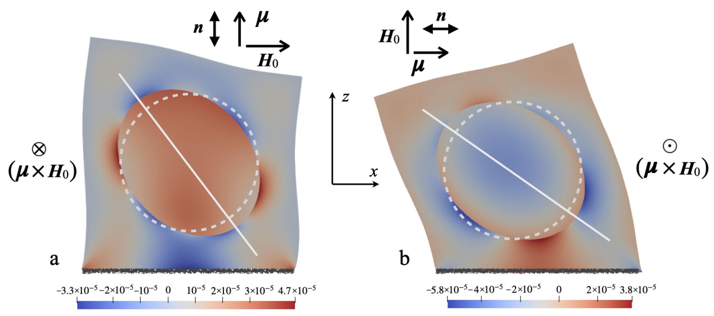
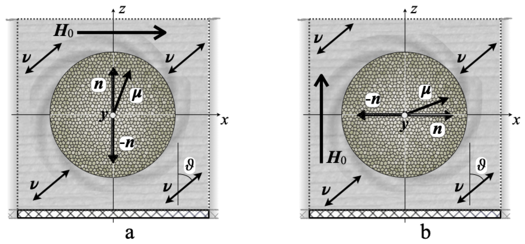
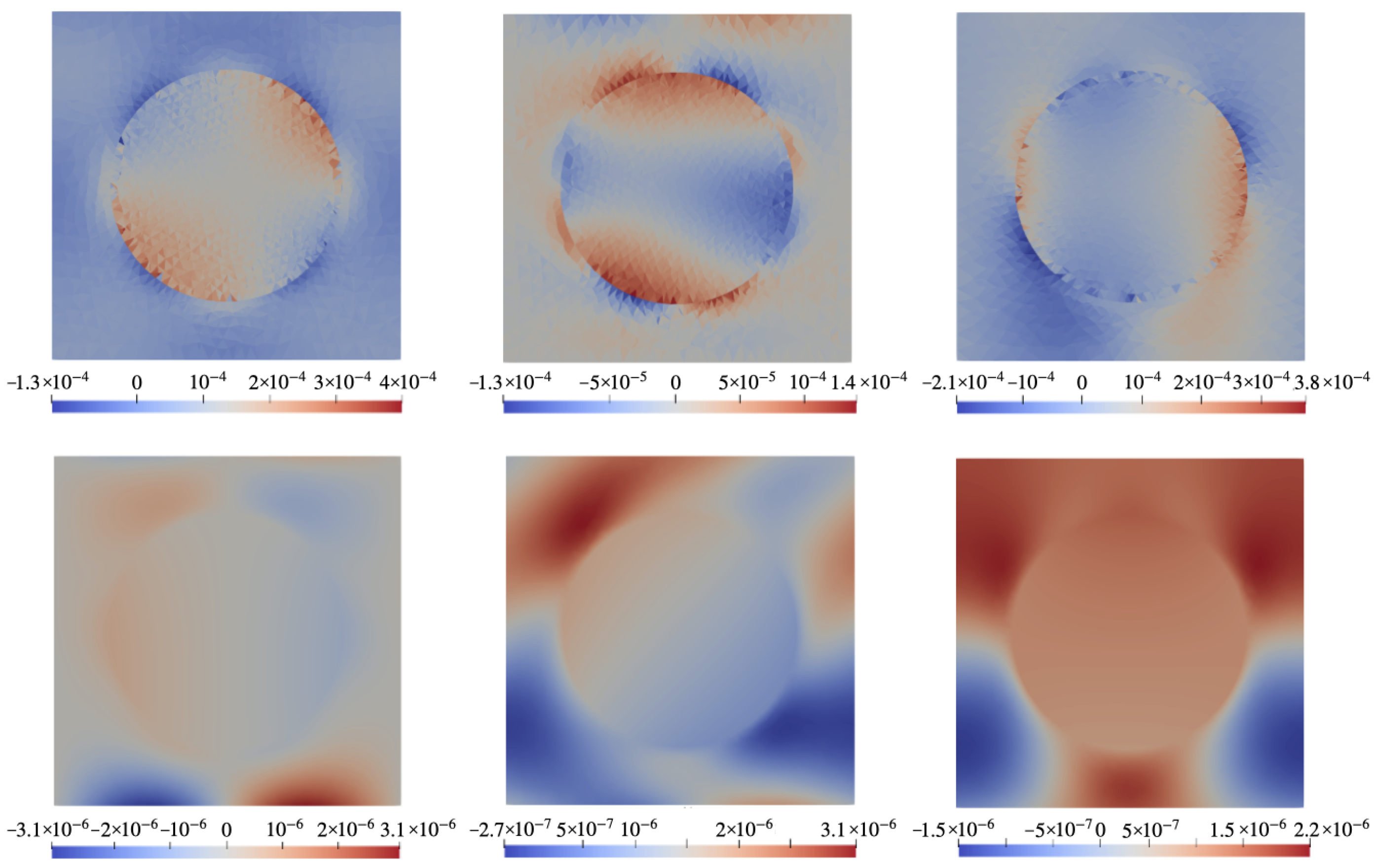
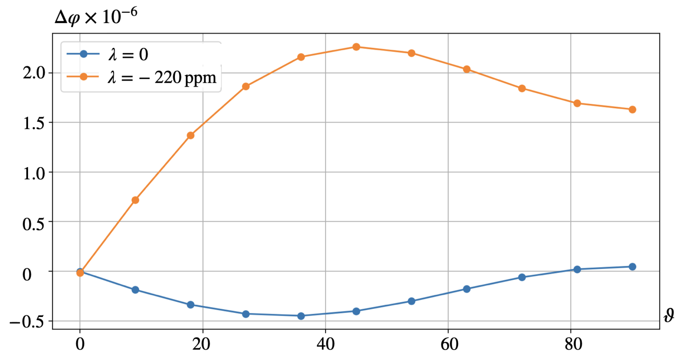
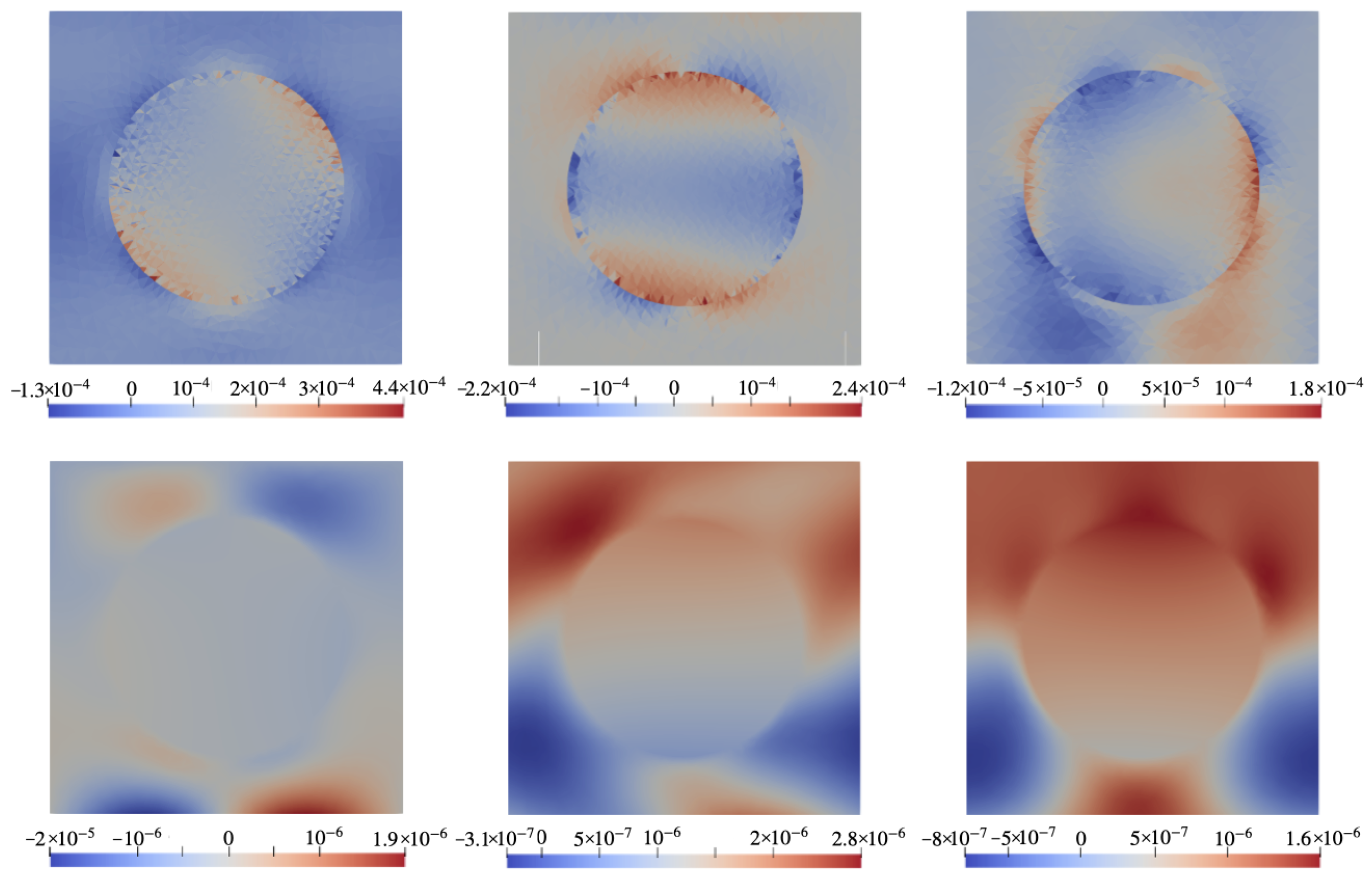
6.1. Configuration A

Figure 3 demonstrates the color maps of mechanical stresses and electric potential $\phi$ (defined against infinity) in the $xOz$ cross-section of the cell of the configuration of Figure 2a) for a ferromagnet with the magnetostriction constant ${\lambda }_s=-220$ ppm. The top row shows the distributions of three components of the stress tensor in the field $H_0=0.01$ pointing along $Ox$. The bottom row presents the distributions of electric potential in the same plane for different orientations of the piezoelectric anisotropy axis (poling direction). Whereas the mechanical stresses do not depend on the direction of vector $\mathit{\nu }$, the induced electric fields are essentially defined by that parameter since in each case the electric polarization is induced via different components of piezotensor $\mathbf{d}$. Note that when evaluating internal magnetic fields, our calculation fully accounts for the demagnetizing fields inside the film.

Figure 4 is the analog of Figure 3 but for a particle made of a hypothetical ferromagnet with magnetostriction constant ${\lambda }_s=0$. As seen from the comparison, the distributions obtained for ${\lambda }_s\ne 0$ and ${\lambda }_s=0$ are drastically different. In this connection, it is important to note that Figure 3 presents the case of joint action of the magnetostriction and magnetic rotation of the particle whereas Figure 4 accounts for the case where only the magnetorotational effect takes part in generation of the electric response.

The bottom rows of Figure 3 and Figure 4 reveal that the distributions of electric potential $\phi$ strongly depend on the poling direction. A full view of this dependence is rendered by Figure 5 where not $\phi$ itself but the difference $\mathsf{\Delta }\phi$ between the values of potential (averaged over the corresponding surface of the representing cell) at the opposite sides of the film is plotted. As it shows, the best results are attained when $\mathit{\nu }$ is oriented under $35÷{45}^{\circ }$ where both contributions are maximal. This takes place despite that the magnetorotational part (the lower curve) is negative in virtually all the angle intervals, reaching the maximum of about 20% of the magnetostrictive one. This evidences that a simple consideration presented in Figure 1a is indeed entirely correct in the qualitative aspect.

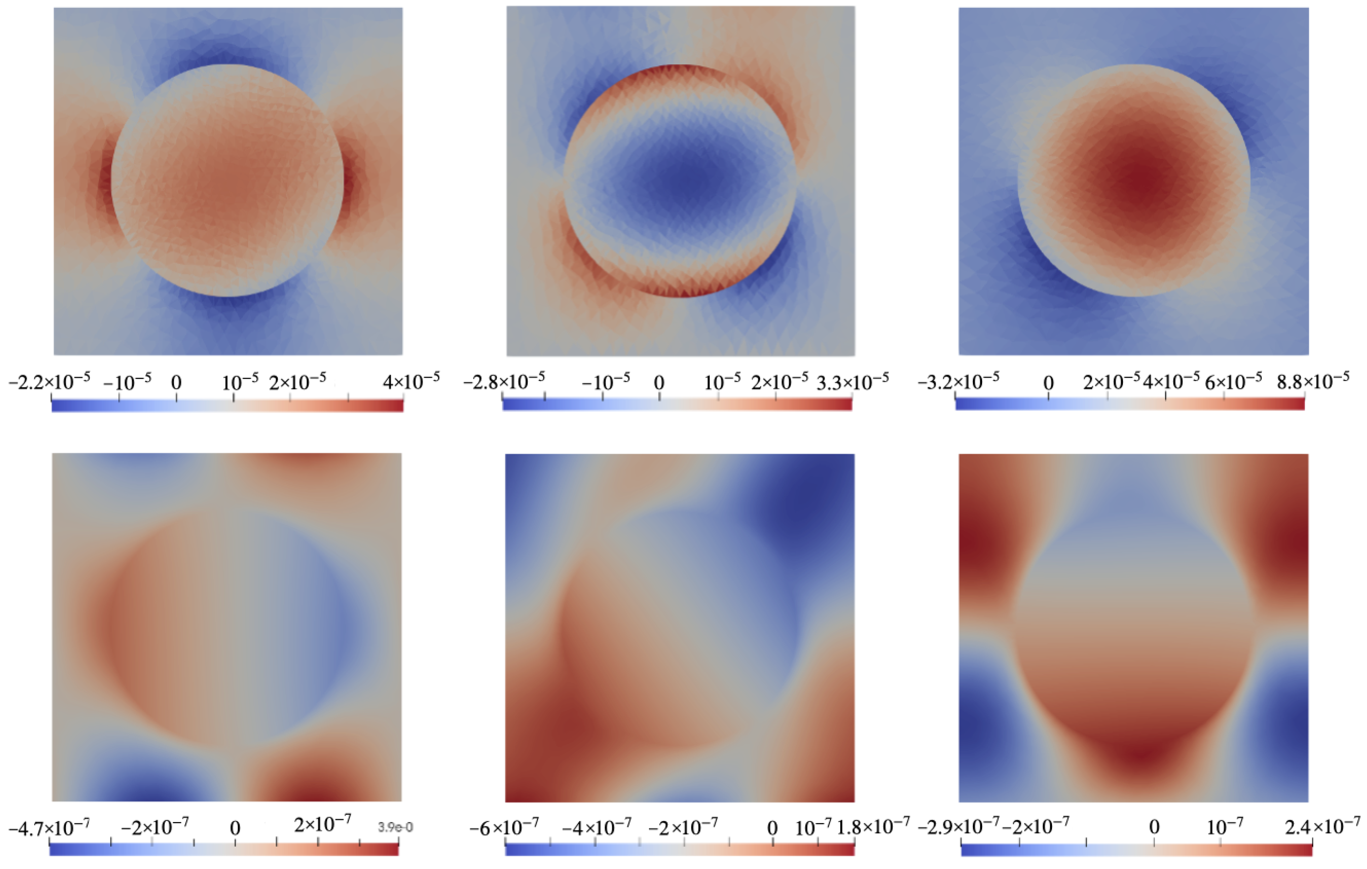
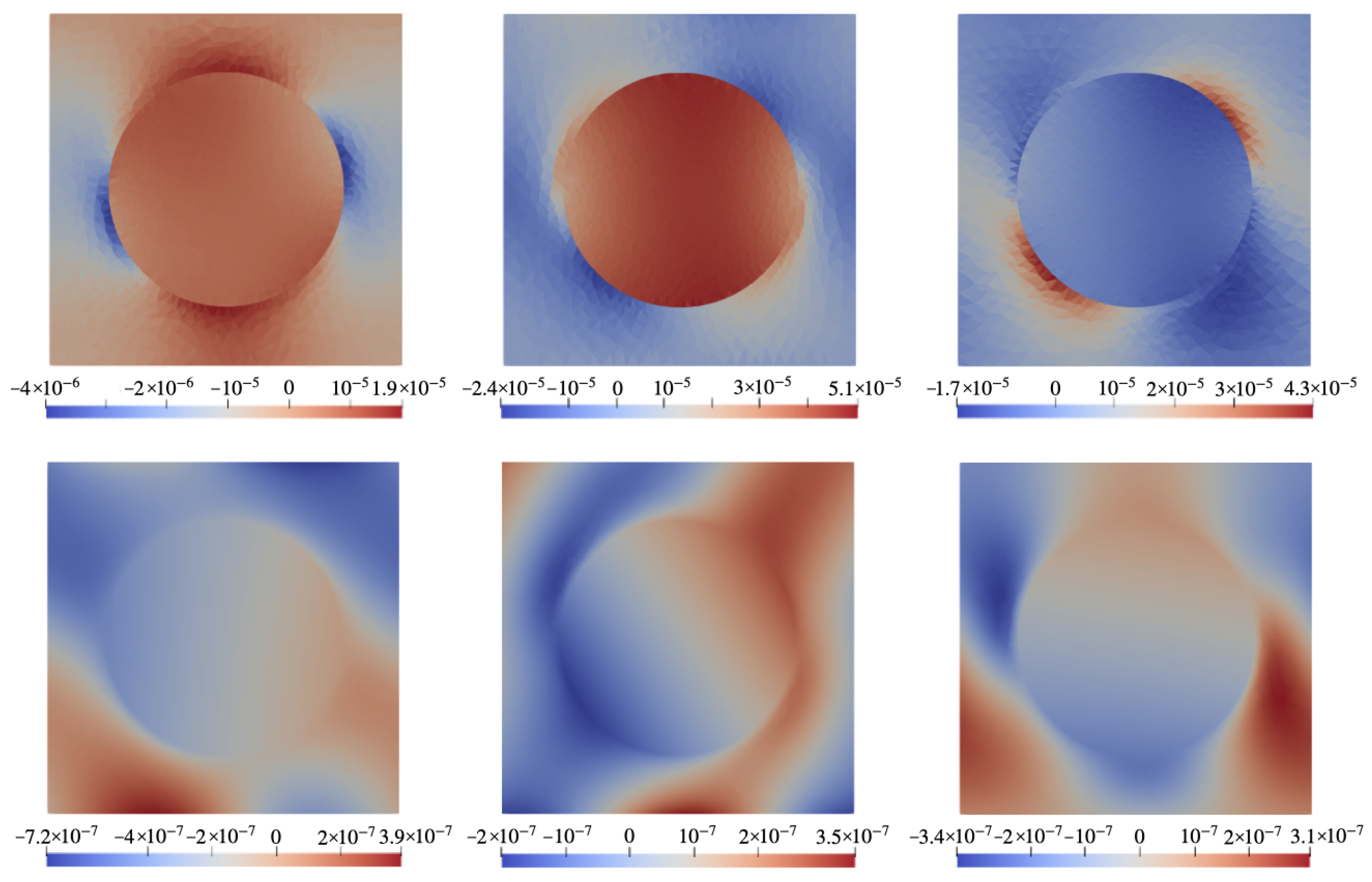
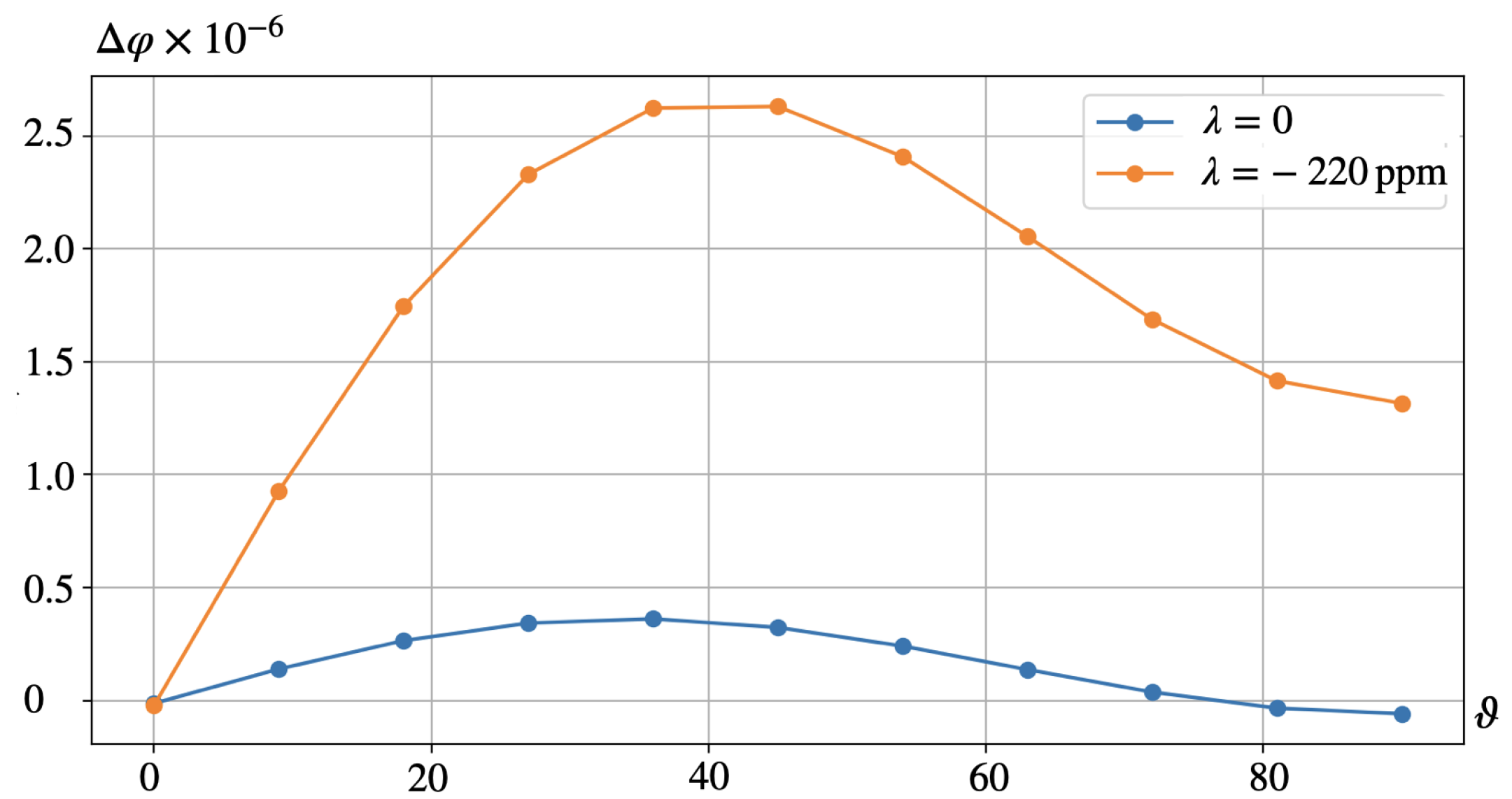
6.2. Configuration B

In Figure 6 the color maps rendering spatial distributions of stresses and electric potential (defined with respect to infinity) in the $xOz$ cross-section of the representing cell in configuration B (see Figure 2b) for a system that contains a particle with magnetostriction constant $\lambda =-220$ ppm. The top row shows three main components of the stress tensor under field $H_0=0.01$ directed along $Oz$. The bottom row presents the spatial distribution of electric potential $\phi$ for different poling directions.

In case B, as in case A, Figure 7 is the analog of Figure 6 for a particle made of a hypothetical ferromagnet whose magnetostriction constant is identical zero. In this connection, we again note that Figure 6 presents the case of joint action of the magnetostriction and magnetic rotation of the particle whereas Figure 7 describes the case where the electric response is due solely to the magnetorotational effect. Quite expectedly, the bottom rows of Figure 6 and Figure 7, when compared, evidence that the distributions of electric potential $\phi$ obtained for the cases of ${\lambda }_s\ne 0$ and ${\lambda }_s=0$ are drastically different and depend strongly on the poling direction. A full view of this dependence is rendered in Figure 8 where the difference $\mathsf{\Delta }\phi$ between the values of $\phi$ (averaged over the corresponding surface of the representing cell) at the opposite faces of the film is plotted. This figure shows that the best results correspond to the orientation range of $\mathit{\nu }$ from ${35}^{\circ }$ to ${45}^{\circ }$ where both contributions are positive and maximal; there the magnetorotational part makes about 20% of the magnetostrictive one. Recalling Figure 1, its panel (b), one finds that that simple illustration provides an entirely correct qualitative prediction.

7. Discussion

The results presented in Section 6 show that numerical simulations confirm the qualitative conclusions drawn in Section 2: depending on the magnetic and piezoelectric orientational textures established in the composite, the magentostrictive and magnetoactive (magnetorotational) mechanisms might either enhance or diminish their joint effect. Indeed, the magnetorotational contribution has opposite signs in A and B configurations whereas the magnetostrictive contributions are always positive. This explains why the obtained electric response $\mathsf{\Delta }\phi$ in configuration B is about 20% higher than in that in configuration A.

It is instructive to compare the relative magnitudes of the two considered effects. A rough estimation may be deduced from comparing the magnetostrictive and magnetorotational torques that develop under the same applied field. We note that for small deviation angles, the magnetorotational torque is

$$Q_{\mathrm{m}.\mathrm{rot}}\sim \left|(\mathit{\mu }·{\mathit{H}}_0)\right|\sim M_{s}v{H}_0,$$

(11)

where v is the particle volume.

The magnetostrictve torque is produced by the particle shape change. From expression (A22) it follows that the magnetostriction strain under $H_0<\frac{1}{2}{H}_A$ is $e^{\left(\mathrm{strict}\right)}\sim 2(H_0/H_A){\lambda }_s$. Then the energy excess and, thus, the torque which, due to magnetostriction, the particle exerts on the matrix is

$$Q_{\mathrm{m}.\mathrm{strict}}\sim |{\mathbf{e}}^{\left(\mathrm{strict}\right)}|E_{\mathrm{p}}v\sim \left|{\lambda }_s\right|E_{\mathrm{p}}v.$$

(12)

Taking the ratio, one finds

$$\xi \equiv Q_{\mathrm{m}.\mathrm{rot}}/Q_{\mathrm{m}.\mathrm{strict}}\sim M_s{H}_A/2\left|{\lambda }_s\right|E_{\mathrm{p}};$$

(13)

note that this estimation does not depend on the particle size.

The reference values for the material parameters used in our calculations are given in Section 4. Substituting these numbers in (13) one finds $\xi$∼0.2 that fairly well agrees with the results of numerical modeling presented in Figure 5 and Figure 8. However, as Equation (13) is based on rather rough assumptions, one should not overestimate the occurred closeness; much more important is that it yields a correct order of magnitude.

More important is that Equation (13) renders the parameter dependences which point out the relative roles of the effects. For instance, it predicts that under lower values of ${\lambda }_s$, like those for magnetite Fe${}_3$O${}_4$ (${\lambda }_s\sim 17÷170$ ppm [33,34,35]) or NdFeB (${\lambda }_s\approx 90$ ppm [36]), let alone barium ferrite BaFe${}_{12}$O${}_{19}$ (${\lambda }_s\approx 9$ ppm [37]), the magnetorotational mechanism of generating the electric response may become fully comparable with the magnetostrictive one and even exceed the effect of the latter. The same enhancement might be encountered as well if to deal with softer polymer matrices, like those of specially prepared PVDF films whose Young moduli range $0.5÷1.3$ GPa, see [14,38]. Besides that, under a fixed direction of the applied field, even the sign of the effect might change, see the curves in Figure 5.

Finally, we proceed to the magnitude of the modeled effects in dimensional form. The expressions of Section 4 yield $\mathsf{\Delta }\overline{\phi }=\overline{\mathcal{E}}·\overline{\mathsf{\ell }}=(g/R)\mathcal{E}\mathsf{\ell }=(g/R)\mathsf{\Delta }\phi$. Setting the size of the magnetic particle to $R\approx 15$ nm and given $\mathsf{\Delta }\overline{\phi }\sim 2\times {10}^{-6}$, one finds

$$\mathsf{\Delta }\phi \sim (R/g)\mathsf{\Delta }\overline{\phi }\sim {10}^{-5}\mathrm{V}\approx 100\mathsf{\mu }\mathrm{V}.$$

(14)

Using this for estimating the magnetoelectric susceptibility of the considered film, one obtains

$${\alpha }_V=\mathsf{\Delta }\phi /(\mathsf{\ell }·H_0)\approx 20\mathrm{mV}/\mathrm{cm}·\mathrm{Oe}.$$

(15)

The obtained value is by no means a very high one if to just directly compare it to the scale of units or tens of volts attained in sensing and harvesting ME devices. However, when assessing this result of Equation (15), one has to put it in a different context. Indeed, the very statement of the above-solved problem applies not to the resonance regimes of cantilever-type setups but to quasi-static situations which are customary for experimental tests on stimulated cell development, i.e., tissue engineering.

Going along this line, we recall that in our simulations the volume fraction of CFO is ${\varphi }_{\mathrm{v}}\sim 0.15$ that, when recalculated to weight content for ${\rho }_{\mathrm{CFO}}\sim 5$ and ${\rho }_{\mathrm{PVDF}}\sim 2$ g/cm${}^3$, yields ${\varphi }_{\mathrm{w}}\sim 0.3$. If to consider a film with weight content ${\varphi }_{\mathrm{w}}\sim 0.1$ that is typical for the biologically-oriented ME films [39], one arrives at ${\alpha }_V\sim 7$ mV/cm·Oe. This value agrees well with the result reported in Ref. [39], where it had been found that a CFO/PVDF film with ${\varphi }_{\mathrm{w}}\sim 0.1$ yields ${\alpha }_V\approx 6.5$ mV/cm·Oe.

8. Conclusions

The major idea of our consideration is to emphasize that the ME effect in polymer composites with magnetically hard particles always comprises at least two contributions of different origins, namely, the magnetostrictive and the magnetoactive (magnetorotational) ones. Mesoscopic modeling seems an adequate way to justify this conclusion since it is capable of describing in detail the mechanical and electromagnetic fields that an applied magnetic field induces inside a composite. As a convenient example of a particular sample, a film is chosen due to its simple overall geometry. To make the calculation comparable, at least qualitatively, with experimental evidence, the ingredients of the model composite are ascribed the properties of a typical pair: the filler particles possess the material parameters inherent to CFO whereas the matrix piezoelectric and mechanical properties are those typical for PVDF. In our view, the results obtained confirm the basic idea of the coexistence of the two above-mentioned polarization-inducing effects. Besides, some signatures had been found in experiments but never accounted for explicitly. This makes it interesting to really measure those effects as separate contributions.

In connection with the subject under discussion, the idea of developing a purely magnetoactive (magnetorotational) magnetoelectric turns up and may be assessed. However, as our simulations predict such a prospect seems rather futile. Meanwhile, given that coexistence of the two above-mentioned ME effects is essential, it looks reasonable to use modelling for adjusting the content and texture of the composite in such a way that both effects would work in optimal proportion. Finally, the internal structure of the composite studied in the present work is too simple to be directly compared with the experiment in any quantitative way. On the other hand, the capabilities of the developed mesoscopic approach are evident. In our future work, we plan to gradually proceed with this toolbox to more complex problems of structural magneto-electro-mechanics of polymer composites.

References

1. Liang, X.; Matyushov, A.; Hayes, P.; Schell, V.; Dong, C.; Chen, H.; He, Y.; Will-Cole, A.; Quandt, E.; Martins, P.; et al. Roadmap on magnetoelectric materials and devices. IEEE Trans. Magn. 2021, 57, 400157. [Google Scholar] [CrossRef]
2. Fernandes, C.L.; Correia, D.M.; Tariq, M.; Esperança, J.M.S.S.; Martins, P.; Lanceros-Méndez, S. Multifunctional magnetoelectric sensing and bending actuator response of polymer-based hybrid materials with magnetic ionic liquids. Nanomaterials 2023, 13, 2186. [Google Scholar] [CrossRef] [PubMed]
3. Zhang, J.; Meng, X.; Fu, G.; Han, T.; Xu, F.; Putson, C.; Liu, X. Enhanced polarization effect of flexible magnetoelectric PVDF-TrFE/Fe3O4 smart nanocomposites for nonvolatile memory application. ACS Appl. Electron. Mater. 2023, 5, 1844–1852. [Google Scholar] [CrossRef]
4. Pourhosseiniasl, M.; Gao, X.; Kamalisiahroudi, S.; Yu, Z.; Chu, Z.; Yang, J.; Lee, H.; Dong, S. Versatile power and energy conversion of magnetoelectric composite materials with high efficiency via electromechanical resonance. NanoEnergy 2020, 70, 104506. [Google Scholar] [CrossRef]
5. Jiang, J.; Liu, S.; Feng, L.; Zhao, D. A review of piezoelectric vibration energy harvesting with magnetic coupling based on different structural characteristics. Micromachines 2021, 12, 436. [Google Scholar] [CrossRef] [PubMed]
6. Sasmal, A.; Sen, S.; Chelvane, J.A.; Arockiarajan, A. PVDF based flexible magnetoelectric composites for capacitive energy storage, hybrid mechanical energy harvesting and self-powered magnetic field detection. Polymer 2023, 281, 126141. [Google Scholar] [CrossRef]
7. Díaz, E.; Valle, M.B.; Ribeiro, S.; Lanceros-Méndez, S.; Barandiarán, J.M. Development of magnetically active scaffolds for bone regeneration. Nanomaterials 2018, 8, 678. [Google Scholar] [CrossRef]
8. Kapat, K.; Shubhra, Q.T.H.; Zhou, M.; Leeuwenburgh, S. Piezoelectric nano-biomaterials for biomedicine and tissue regeneration. Adv. Funct. Mater. 2020, 30, 19009045. [Google Scholar] [CrossRef]
9. Kopyl, S.; Surmenev, R.; Surmeneva, M.; Fetisov, Y.; Kholkin, A. Magnetoelectric effect: Principles and applications in biology and medicine—A review. Mater. Today Bio 2021, 12, 100149. [Google Scholar] [CrossRef]
10. Silva, C.A.; Fernandes, M.M.; Ribeiro, C.; Lanceros-Méndez, S. Two- and three-dimensional piezoelectric scaffolds for bone tissue engineering. Colloids Surfaces B Biointerfaces 2022, 218, 112708. [Google Scholar] [CrossRef]
11. Zhao, H.; Liu, C.; Liu, Y.; Ding, Q.; Wang, T.; Li, H.; Wu, H.; Ma, T. Harnessing electromagnetic fields to assist bone tissue engineering. Stem Cell Res. Ther. 2023, 14, 7. [Google Scholar] [CrossRef] [PubMed]
12. Sharma, M.; Madras, G.; Bose, S. Process induced electroactive polymorph in PVDF: Effect on dielectric and ferroelectric properties. Phys. Chem. Chem. Phys. 2014, 16, 14792–14799. [Google Scholar] [CrossRef] [PubMed]
13. Ruan, L.; Yao, X.; Chang, Y.; Zhou, L.; Qin, G.; Zhang, X. Properties and applications of the β phase poly(vinylidene fluoride). Polymers 2018, 10, 228. [Google Scholar] [CrossRef] [PubMed]
14. Nivedhitha, D.M.; Subramanian, J. Polyvinylidene fluoride, an advanced futuristic smart polymer material: A comprehensive review. Polym. Adv. Technol. 2023, 34, 474–505. [Google Scholar] [CrossRef]
15. Correia, D.M.; Gonçalves, R.; Ribeiro, C.; Sencadas, V.; Botelho, G.; Ribelles, J.G.; Lanceros-Méndez, S. Electrosprayed poly(vinylidene fluoride) microparticles for tissue engineering applications. RSC Adv. 2014, 4, 33013–33021. [Google Scholar] [CrossRef]
16. Gonçalves, R.; Martins, P.; Correia, D.M.; Sencadas, V.; Vilas, J.L.; León, L.M.; Botelho, G.; Lanceros-Méndez, S. Development of magnetoelectric CoFe2O4/poly(vinylidene fluoride) microspheres. RSC Adv. 2015, 5, 35852–35857. [Google Scholar] [CrossRef]
17. Omelyanchik, A.; Antipova, V.; Gritsenko, C.; Kolesnikova, V.; Murzin, D.; Han, Y.; Turutin, A.V.; Kubasov, I.V.; Kislyuk, A.M.; Ilina, T.S.; et al. Boosting magnetoelectric effect in polymer-based nanocomposites. Nanomaterials 2021, 11, 1154. [Google Scholar] [CrossRef]
18. Martins, L.A.; Ródenas-Rochina, J.; Salazar, D.; Cardoso, V.F.; Ribelles, J.L.G.; Lanceros-Méndez, S. Microfluidic processing of piezoelectric and magnetic responsive electroactive microspheres. ACS Appl. Polym. Mater. 2017, 4, 5368–5379. [Google Scholar] [CrossRef]
19. Stolbov, O.V.; Ignatov, A.A.; Rodionova, V.V.; Raikher, Y.L. Modelling the effect of particle arrangement on the magnetoelectric response of a polymer multiferroic film. Soft Matter 2023, 19, 4029–4040. [Google Scholar] [CrossRef]
20. Martins, P.; Larrea, A.; Gonçalves, R.; Botelho, G.; Ramana, E.V.; Mendiratta, S.K.; Sebastian, V.; Lanceros-Méndez, S. Novel anisotropic magnetoelectric effect on #-FeO(OH)/P(VDF-TrFE) multiferroic composites. ACS Appl. Mater. Interfaces 2015, 7, 1122–1129. [Google Scholar] [CrossRef]
21. Gutiérrez, J.; Martins, P.; Gonçalves, R.; Sencadas, V.; Lasheras, A.; Lanceros-Méndez, S.; Barandiarán, J.M. Synthesis, physical and magnetic properties of BaFe12O19 / P(VDF-TrFE) multifunctional composites. Eur. Polym. J. 2015, 69, 224–231. [Google Scholar] [CrossRef]
22. Anithakumari, P.; Mandal, B.P.; Abdelhamid, E.; Naik, R.; Tyagi, A.K. Enhancement of dielectric, ferroelectric and magneto-dielectric properties in PVDF-BaFe12O19 composites. RSC Adv. 2016, 6, 16073–16080. [Google Scholar] [CrossRef]
23. Gonçalves, R.; Larrea, A.; Zheng, T.; Higgins, M.J.; Sebastian, V.; Lanceros-Méndez, S.; Martins, P. Synthesis of highly magnetostrictive nanostructures and their application in a polymer-based magnetoelectric sensing device. Eur. Polym. J. 2016, 84, 685–692. [Google Scholar] [CrossRef]
24. Alnassar, M.Y.; Ivanov, Y.P.; Kosel, J. Flexible magnetoelectric nanocomposites with tunable properties. Adv. Electron. Mater. 2016, 2, 1600081. [Google Scholar] [CrossRef]
25. Nan, C.-W.; Bichurin, M.I.; Dong, S.; Viehland, D.; Srinivasan, G. Multiferroic magnetoelectric composites: Historical perspective, status, and future directions. J. Appl. Phys. 2008, 103, 031101. [Google Scholar] [CrossRef]
26. Ma, J.; Hu, J.; Li, Z.; Nan, C.-W. Recent progress in multiferroic magnetoelectric composites: From bulk to thin films. Adv. Mater. 2011, 23, 1062–1087. [Google Scholar] [CrossRef]
27. Acosta, M.; Novak, N.; Rojas, V.; Patel, S.; Vaish, R.; Koruza, J.; Rossetti, G.A.; Rödel, J. BaTiO3-based piezoelectrics: Fundamentals, current status, and perspectives. Appl. Phys. Rev. 2018, 4, 041305. [Google Scholar] [CrossRef]
28. Ferson, N.D.; Uhl, A.M.; Andrew, J.S. Piezoelectric and magnetoelectric scaffolds for tissue regeneration and biomedicine: A Review. IEEE Trans. Ultrason. Ferroelectr. Freq. Control 2020, 68, 229–241. [Google Scholar] [CrossRef]
29. Meng, Y.; Chen, G.; Huang, M. Piezoelectric materials: Properties, advancements, and design strategies for high-temperature applications. Nanomaterials 2022, 12, 1171. [Google Scholar] [CrossRef]
30. Zhang, J.; Chen, X.; Wang, X.; Fang, C.; Weng, G.J. Magnetic, mechanical, electrical properties and coupling effects of particle reinforced piezoelectric polymer matrix composites. Compos. Struct. 2022, 304, 116450. [Google Scholar] [CrossRef]
31. Landau, L.D.; Lifshitz, E.M. Electrodynamics of Continuous Media, 2nd ed.; Elsevier: Amsterdam, The Netherlands, 1984. [Google Scholar]
32. FEniCS Project. Available online: http://www.fenicsproject.org (accessed on 8 September 2023).
33. Bickford, L.R.; Pappis, J.; Stull, J.L. Magnetostriction and permeability of magnetite and cobalt-substituted magnetite. Phys. Rev. 1955, 99, 1210–1214. [Google Scholar] [CrossRef]
34. Bozort, R.M.; Tilden, E.F.; Williams, A.J. Anisotropy and magnetostriction of some ferrites. Phys. Rev. 1955, 99, 1788–1798. [Google Scholar] [CrossRef]
35. Gonçalves, R.; Larrea, A.; Sebastian, M.S.; Sebastian, V.; Martins, P.; Lanceros-Méndez, S. Synthesis and size dependent magnetostrictive response of ferrite nanoparticles and their application on magnetoelectric polymer-based multiferroic sensors. J. Mater. Chem. C 2016, 4, 10701–10706. [Google Scholar] [CrossRef]
36. de Groot, C.H.; de Kort, K. Magnetoelastic anisotropy in NdFeB permanent magnets. J. Appl. Phys. 1999, 85, 8312–8316. [Google Scholar] [CrossRef]
37. Licei, F.; Rinaldi, S. Magnetostriction of some hexagonal ferrites. J. Appl. Phys. 1981, 52, 2442–2443. [Google Scholar] [CrossRef]
38. Cui, Y.; Sui, Y.; Wei, P.; Lv, Y.; Cong, C.; Meng, X.; Ye, H.; Zhou, Q. Rationalizing the dependence of poly (vinylidene difluoride) (PVDF) rheological performance on the nano-silica. Nanomaterials 2023, 13, 1096. [Google Scholar] [CrossRef]
39. Tang, B.; Zhuang, J.; Wang, L.; Zhang, B.; Lin, S.; Jia, F.; Dong, L.; Wang, Q.; Cheng, K.; Weng, W. Harnessing cell dynamic responses on magnetoelectric nanocomposite films to promote osteogenic differentiation. ACS Appl. Mater. Interfaces 2018, 10, 7841–7851. [Google Scholar] [CrossRef]
40. Bustamante, R.; Dorfmann, A.; Ogden, R.W. On boundary conditions in nonlinear magneto- and electroelasticity. In Constitutive Models for Rubber; Balkema-Proceedings and Monographs in Engineering, Water, and Earth Sciences; Boukamel, A., Laiarinandrasana, L., Meo, S., Verron, E., Eds.; Taylor & Francis: London, UK, 2008; Volume 5, pp. 339–344. [Google Scholar]
41. Ogden, R.W. Non-Linear Elastic Deformations; Dover: New York, NY, USA, 1984. [Google Scholar]
42. Ueberschlag, P. PVDF piezoelectric polymer. Sens. Rev. 2001, 21, 118–125. [Google Scholar] [CrossRef]
Figure 1. A 2D cell that comprises a single-domain uniaxial particle experiencing the joint action of magnetostrictive and magnetorotational effects; white lines mark the direction of the long axis of the striction-deformed particle. The color renders the shear stress distributions, the corresponding strains are enhanced by 10 5 against the spatial scale of the figure. Panels (a) and (b) differ by the relative positions of μ and H 0 vectors and, hence, the direction of the magnetic torque.
Nanomaterials 14 00031 g001
Figure 2. Schematic cross-sections of the elementary cubic cell for two variants of the initial position of the particle; panels (a) and (b) differ by the orientation of the applied field and magnetic anisotropy axis of the particle relative to the film plane; angle ϑ denotes the poling direction ν .
Nanomaterials 14 00031 g002
Figure 3. Color maps of mechanical stress σ and electric potential φ in x O z plane of the cell with configuration A (Figure 2a) under field H 0 = 0.01 directed along O x for a CFO-like particle with λ s = 220 ppm. Top row: components σ x z (left), σ x x (center), σ z z (right); bottom row: electric potential φ under poling directions ϑ = 0 (left), 45 (center), 90 (right).
Nanomaterials 14 00031 g003
Figure 4. The same as in Figure 3 for a ferromagnet particle with λ s = 0 .
Nanomaterials 14 00031 g004
Figure 5. Configuration A, see Figure 2a. Dependence of the transverse voltage on the orientation of the piezoelectric axis ν for λ s = 220 ppm and λ s = 0 .
Nanomaterials 14 00031 g005
Figure 6. Color maps of mechanical stress σ and electric potential φ in x O z plane of the cell with configuration B (Figure 2b) under field H 0 = 0.01 directed along O z for a CFO-like particle with λ s = 220 ppm. Top row: components σ x z (left), σ x x (center), σ z z (right); bottom row: electric potential under poling directions ϑ = 0 (left), 45 (center), 90 (right).
Nanomaterials 14 00031 g006
Figure 7. The same as in Figure 6 for a ferromagnet particle with λ s = 0 .
Nanomaterials 14 00031 g007
Figure 8. Configuration B, see Figure 2b. Dependence of the transverse voltage on the orientation of the piezoelectric axis ν for λ s = 220 ppm and λ s = 0 .
Nanomaterials 14 00031 g008
Disclaimer/Publisher’s Note: The statements, opinions and data contained in all publications are solely those of the individual author(s) and contributor(s) and not of MDPI and/or the editor(s). MDPI and/or the editor(s) disclaim responsibility for any injury to people or property resulting from any ideas, methods, instructions or products referred to in the content.