
Magnetic Properties and Magnetocaloric Effect of Polycrystalline and Nano-Manganites Pr0.65Sr(0.35−x)CaxMnO3 (x ≤ 0.3)


Abstract
:1. Introduction
2. Materials and Methods
3. Results
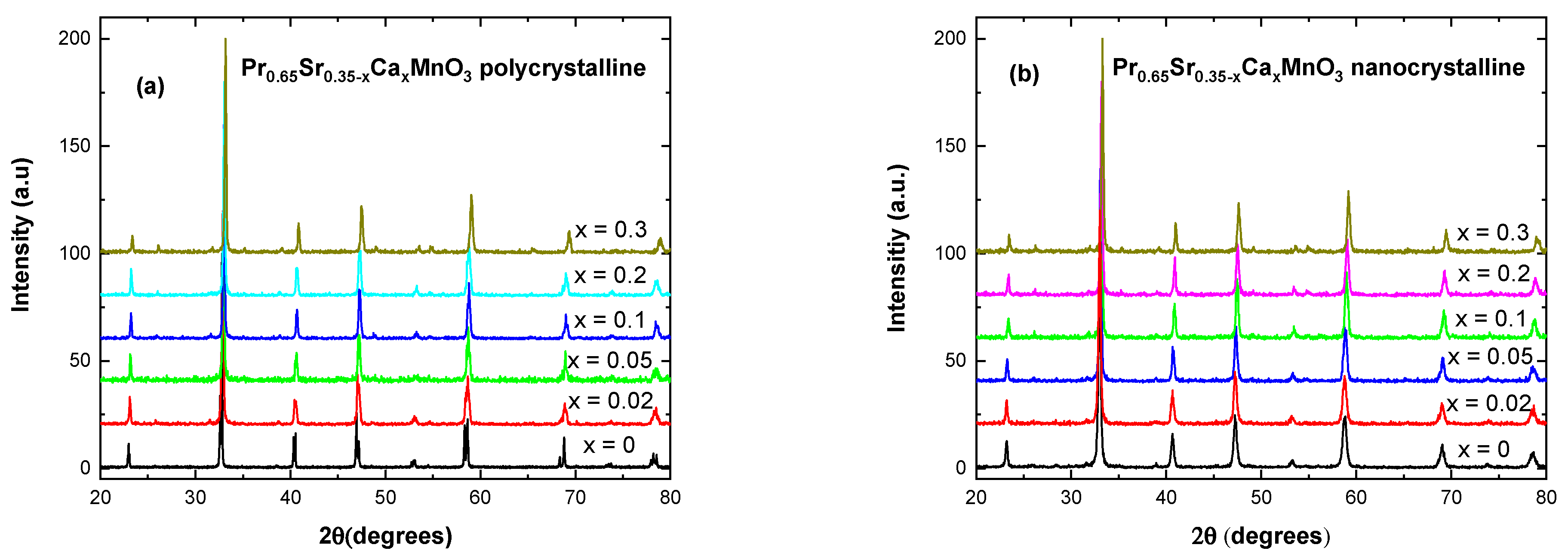
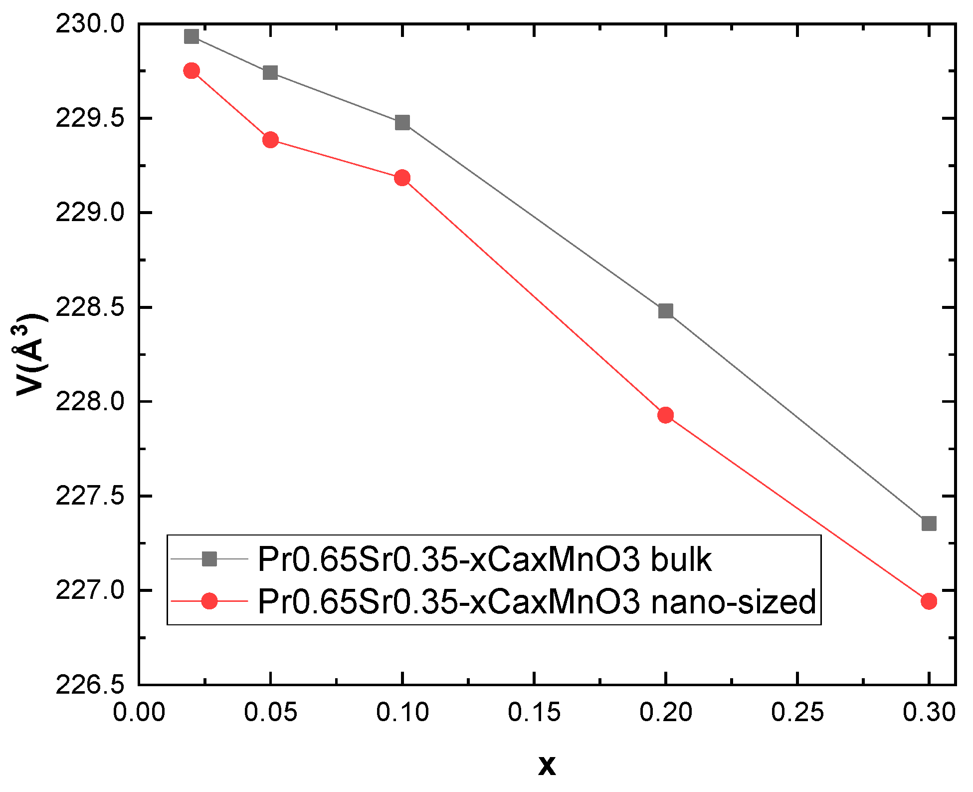
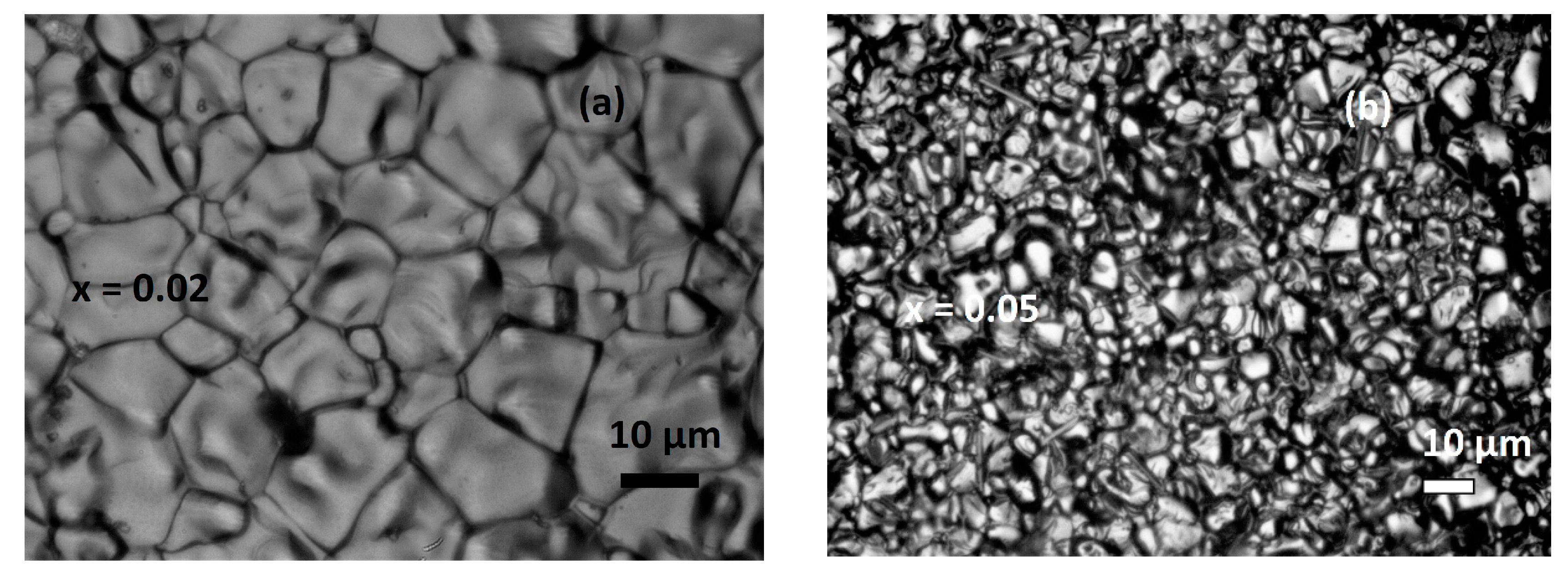
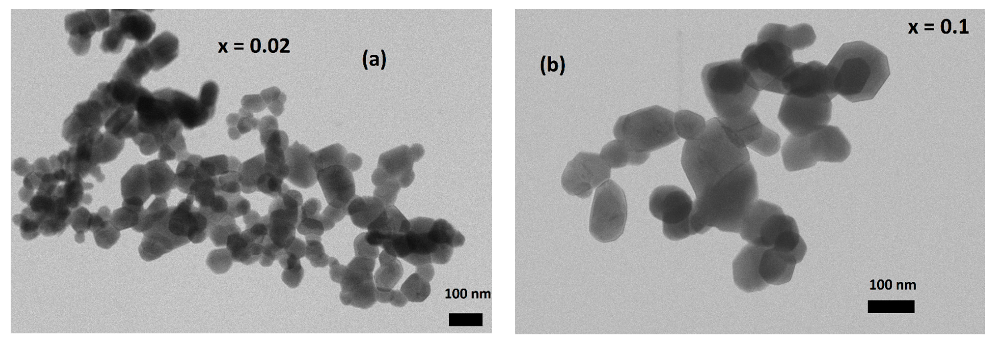
3.1. Structural Analysis
3.2. Oxygen Content
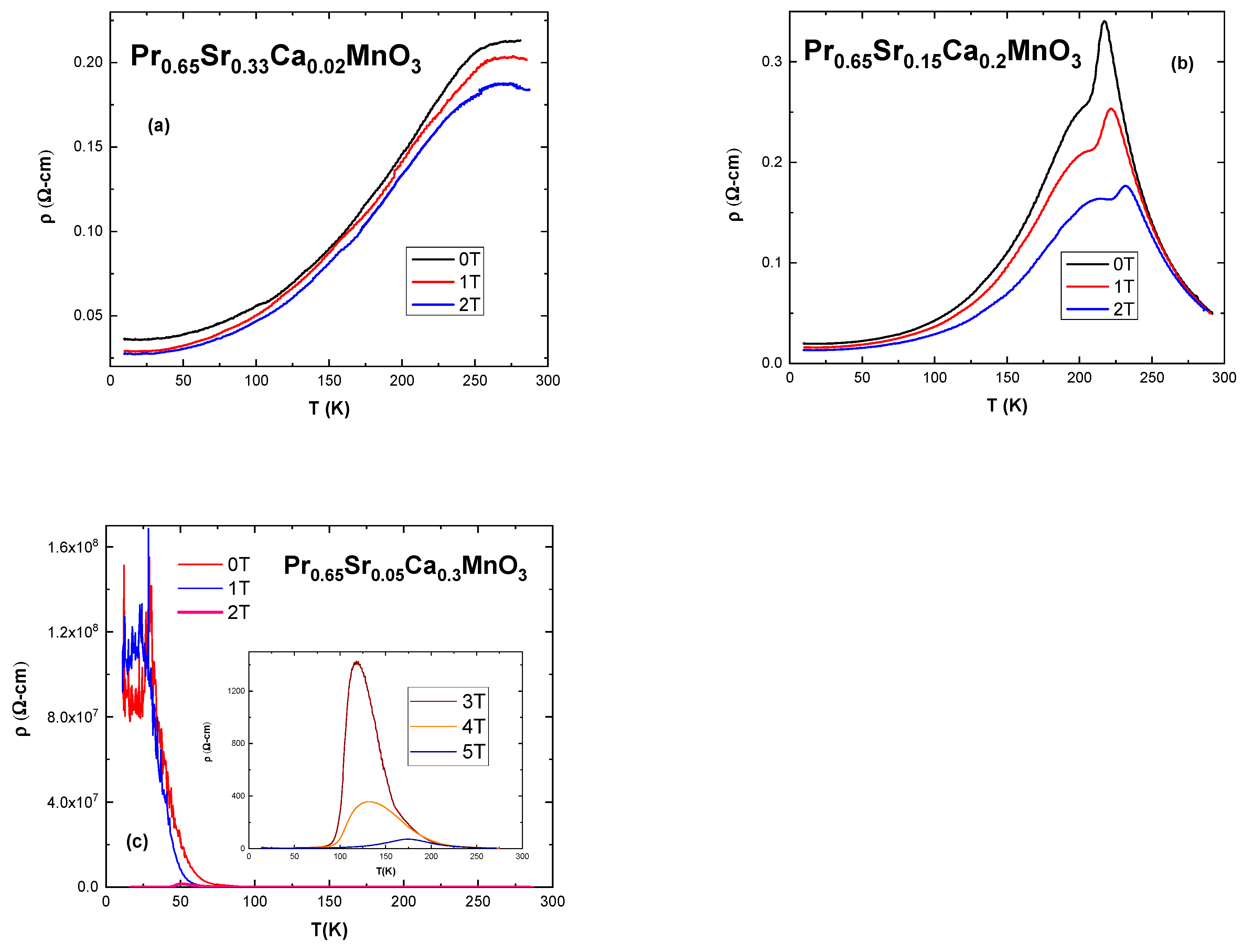
3.3. Electrical Measurements
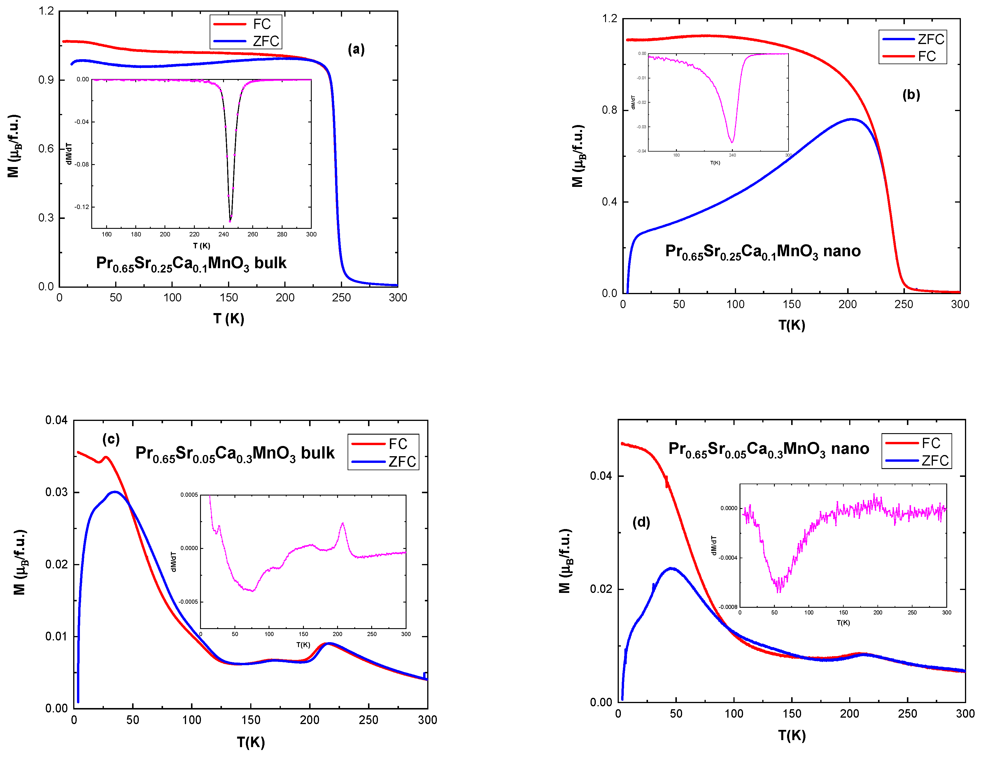
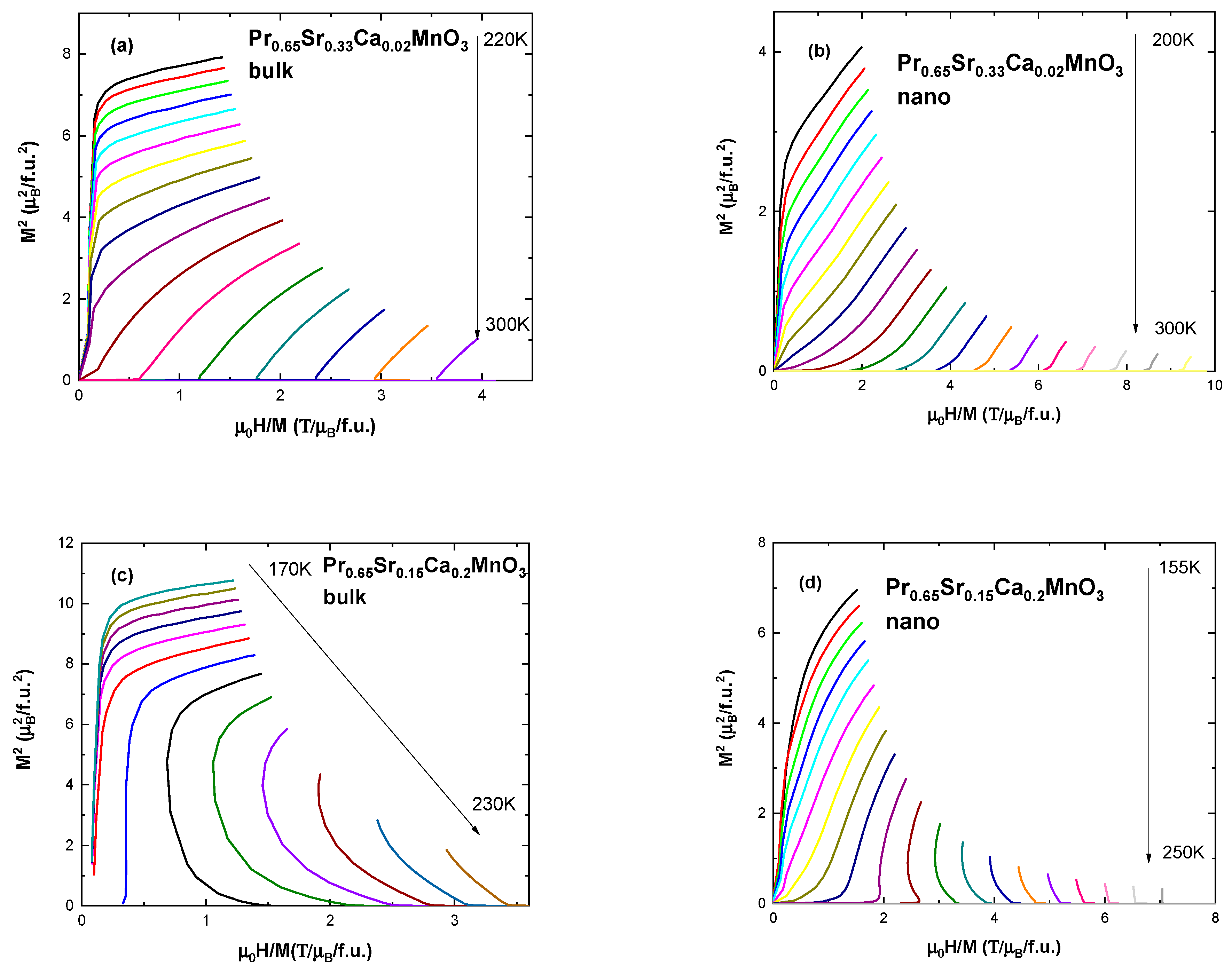
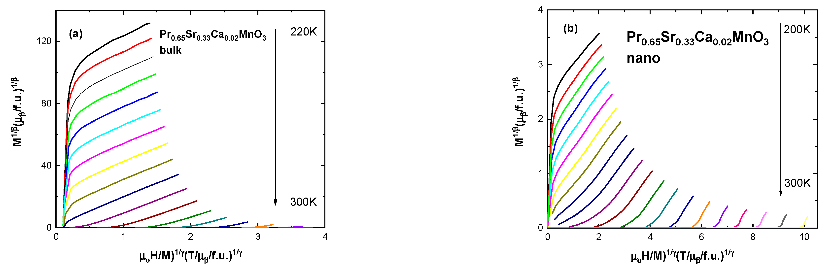
3.4. Magnetic Properties
4. Conclusions
Author Contributions
Funding
Data Availability Statement
Acknowledgments
Conflicts of Interest
References
- Mckay, C.P. Requirements and limits for life in the context of exoplanets. Proc. Natl. Acad. Sci. USA 2014, 111, 12628–12633. [Google Scholar] [CrossRef] [PubMed] [Green Version]
- Briley, G.C. A History of Refrigeration. Ashrae J. 2004, 46, S31–S34. [Google Scholar]
- Gschneidner, K.A.; Pecharsky, V.K. Thirty Years of near Room Temperature Magnetic Cooling: Where We Are Today and Future Prospects. Int. J. Refrig. 2008, 31, 945–961. [Google Scholar] [CrossRef] [Green Version]
- Salazar-Munoz, V.E.; Lobo Guerrero, A.; Palomares-Sanchez, S.A. Review of magnetocaloric properties in lanthanum manganites. J. Magn. Magn. Mater. 2022, 562, 169787. [Google Scholar] [CrossRef]
- Smith, A. Who discovered the magnetocaloric effect? EPJH 2013, 38, 507–517. [Google Scholar] [CrossRef]
- Dagotto, E.; Hotta, T.; Moreo, A. Colossal Magnetoresistant Materials: The Key Role of Phase Separation. Phys. Rep. 2001, 344, 1–153. [Google Scholar] [CrossRef] [Green Version]
- Pavarini, E.; Koch, E.; Anders, F.; Jarrell, M. Correlated Electrons: From Models to Materials Modeling and Simulation; Forschungszentrum Julich: Jülich, Germany, 2012; Chapter 7; Volume 2, pp. 18–21. ISBN 978-3-89336-796-2. [Google Scholar]
- Coey, J.M.D.; Viret, M.; Von Molnár, S. Mixed-Valence Manganites. Adv. Phys. 1999, 48, 167–293. [Google Scholar] [CrossRef]
- Rostamnejadi, A.; Venkatesan, M.; Alaria, J.; Boese, M.; Kameli, P.; Salamati, H.; Coey, J.M.D. Conventional and Inverse Magnetocaloric Effects in La0.45Sr 0.55MnO3 Nanoparticles. J. Appl. Phys. 2011, 110, 043905. [Google Scholar] [CrossRef] [Green Version]
- Varvescu, A.; Deac, I.G. Critical Magnetic Behavior and Large Magnetocaloric Effect in Pr0.67Ba0.33MnO3 Perovskite Manganite. Phys. B Condens. Matter 2015, 470–471, 96–101. [Google Scholar] [CrossRef]
- Badea, C.; Tetean, R.; Deac, I.G. Suppression of Charge and Antiferromagnetic Ordering in Ga-doped La0.4Ca0.6MnO3. Rom. J. Phys. 2018, 63, 604. [Google Scholar]
- Guillou, F.; Legait, U.; Kedous-Lebouc, A.; Hardy, V. Development of a new magnetocaloric material used in a magnetic refrigeration device. EPJ Web Conf. 2012, 29, 21. [Google Scholar] [CrossRef] [Green Version]
- Licci, F.; Turilli, G.; Ferro, P. Determination of Manganese Valence in Complex La-Mn Perovskites. J. Magn. Magn. Mater. 1996, 164, L268–L272. [Google Scholar] [CrossRef]
- Zhang, X.H.; Li, Z.Q.; Song, W.; Du, X.W.; Wu, P.; Bai, H.L.; Jiang, H.Y. Magnetic properties and charge ordering in Pr0.75Na0.25MnO3 manganite. Solid State Commun. 2005, 135, 356. [Google Scholar] [CrossRef]
- Rao, C.N.R. Charge, Spin, and Orbital Ordering in the Perovskite Manganates, Ln1−xAxMnO3 (Ln = Rare Earth, A = Ca or Sr). J. Phys. Chem. B 2000, 104, 5877–5889. [Google Scholar] [CrossRef]
- Tali, R. Determination of Average Oxidation State of Mn in ScMnO3 and CaMnO3 by Using Iodometric Titration. Damascus Univ. J. Basic Sci. 2007, 23, 9–19. [Google Scholar]
- Ehsani, M.H.; Kameli, P.; Ghazi, M.E.; Razavi, F.S.; Taheri, M. Tunable magnetic and magnetocaloric properties of La0.6Sr0.4MnO3 nanoparticles. J. Appl. Phys. 2013, 114, 223907. [Google Scholar] [CrossRef]
- Dagotto, E. Nanoscale Phase Separation and Colossal Magnetoresistance, 1st ed.; Springer Science & Business Media: New York, NY, USA, 2002; pp. 271–284. [Google Scholar]
- Raju, K.; Manjunathrao, S.; Venugopal Reddy, P. Correlation between Charge, Spin and Lattice in La-Eu-Sr Manganites. J. Low Temp. Phys. 2012, 168, 334–349. [Google Scholar] [CrossRef]
- Rao, C.N.R. Perovskites. In Encyclopedia of Physical Science and Technology; Elsevier: Amsterdam, The Netherlands, 2003; pp. 707–714. [Google Scholar]
- Nath, D.; Singh, F.; Das, R. X-ray Diffraction Analysis by Williamson-Hall, Halder-Wagner and Size-Strain Plot Methods of CdSe Nanoparticles—A Comparative Study. Mater. Chem. Phys. 2020, 239, 2764–2772. [Google Scholar] [CrossRef]
- Atanasov, R.; Bortnic, R.; Hirian, R.; Covaci, E.; Frentiu, T.; Popa, F.; Iosif Grigore Deac, I.G. Magnetic and Magnetocaloric Properties of Nano- and Polycrystalline Manganites La(0.7−x)EuxBa0.3MnO3. Materials 2022, 15, 7645. [Google Scholar] [CrossRef]
- Saw, A.K.; Channagoudra, G.; Hunagund, S.; Hadimani, R.L.; Dayal, V. Study of transport, magnetic and magnetocaloric properties in Sr2+ substituted praseodymium manganite. Mater. Res. Express 2020, 7, 016105. [Google Scholar] [CrossRef]
- Deac, I.G.; Tetean, R.; Burzo, E. Phase Separation, Transport and Magnetic Properties of La2/3A1/3Mn1−XCoxO3, A = Ca, Sr (0.5 ≤ x ≤ 1). Phys. B Condens. Matter 2008, 403, 1622–1624. [Google Scholar] [CrossRef]
- Panwar, N.; Pandya, D.K.; Agarwal, S.K. Magneto-Transport and Magnetization Studies of Pr2/3Ba 1/3MnO3:Ag2O Composite Manganites. J. Phys. Condens. Matter 2007, 19, 456224. [Google Scholar] [CrossRef]
- Panwar, N.; Pandya, D.K.; Rao, A.; Wu, K.K.; Kaurav, N.; Kuo, Y.K.; Agarwal, S.K. Electrical and Thermal Properties of Pr 2/3(Ba1−XCsx)1/3MnO 3 Manganites. Eur. Phys. J. B 2008, 65, 179–186. [Google Scholar] [CrossRef]
- Ibrahim, N.; Rusop, N.A.M.; Rozilah, R.; Asmira, N.; Yahya, A.K. Effect of grain modification on electrical transport properties and electroresistance behavior of Sm0.55Sr0.45MnO3. Int. J. Eng. Technol. 2018, 7, 113–117. [Google Scholar]
- Kubo, K.; Ohata, N. A Quantum Theory of Double Exchange. J. Phys. Soc. Jpn. 1972, 33, 21–32. [Google Scholar] [CrossRef]
- Arun, B.; Suneesh, M.V.; Vasundhara, M. Comparative Study of Magnetic Ordering and Electrical Transport in Bulk and Nano-Grained Nd0.67Sr0.33MnO3 Manganites. J. Magn. Magn. Mater. 2016, 418, 265–272. [Google Scholar] [CrossRef]
- Peters, J.A. Relaxivity of Manganese Ferrite Nanoparticles. Prog. Nucl. Magn. Reson. Spectrosc. 2020, 120, 72–94. [Google Scholar] [CrossRef] [PubMed]
- Maheswar Repaka, D.V. Magnetic Control of Spin Entropy, Thermoelectricity and Electrical Resistivity in Selected Manganites. Ph.D. Thesis, National University of Singapore, Singapore, 2014. [Google Scholar]
- Deac, I.G.; Diaz, S.V.; Kim, B.G.; Cheong, S.-W.; Schiffer, P. Magnetic relaxation in La0.250Pr0.375Ca0.375MnO3 with varying phase separation. Phys. Rev. B 2002, 64, 174426. [Google Scholar] [CrossRef] [Green Version]
- Deac, I.G.; Mitchell, J.; Schiffer, P. Phase Separation and the Low-Field Bulk Magnetic Properties of Pr0.7Ca0.3MnO3. Phys. Rev. B 2001, 63, 172408. [Google Scholar] [CrossRef] [Green Version]
- Sudyoadsuka, T.; Suryanarayananb, R.; Winotaia, P.; Wengerc, L.E. Suppression of charge-ordering and appearance of magnetoresistance in a spin-cluster glass manganite La0.3Ca0.7Mn0.8Cr0.2O3. J. Magn. Magn. Mater. 2004, 278, 96–106. [Google Scholar] [CrossRef] [Green Version]
- Anuradha, K.N.; Rao, S.S.; Bhat, S.V. Complete ‘melting’ of charge order in hydrothermally grown Pr0.57Ca0.41Ba0.02MnO3 nanowires. J. Nanosci. Nanotechnol. 2007, 7, 1775–1778. [Google Scholar] [CrossRef] [Green Version]
- Rao, S.S.; Tripathi, S.; Pandey, D.; Bhat, S.V. Suppression of charge order, disappearance of antiferromagnetism, and emergence of ferromagnetism in Nd0.5Ca0.5MnO3 nanoparticles. Phys. Rev. B 2006, 74, 144416. [Google Scholar] [CrossRef]
- Lu, C.L.; Dong, S.; Wang, K.F.; Gao, F.; Li, P.L.; Lv, L.Y.; Liu, J.M. Charge-order breaking and ferromagnetism in La0.4Ca0.6MnO3 nanoparticles. Appl. Phys. Lett. 2007, 91, 032502. [Google Scholar] [CrossRef] [Green Version]
- Hüser, D.; Wenger, L.E.; van Duynevelt, A.J.; Mydosh, J.A. Dynamical behavior of the susceptibility around the freezing temperature in (Eu,Sr)S. Phys. Rev. B 1983, 27, 3100. [Google Scholar] [CrossRef]
- Cao, G.; Zhang, J.; Wang, S.; Yu, J.; Jing, C.; Cao, S.; Shen, X. Reentrant spin glass behavior in CE-type AFM Pr0.5Ca0.5MnO3 manganite. J. Magn. Magn. Mater. 2007, 310, 169. [Google Scholar] [CrossRef]
- Jeddi, M.; Gharsallah, H.; Bejar, M.; Bekri, M.; Dhahri, E.; Hlil, E.K. Magnetocaloric Study, Critical Behavior and Spontaneous Magnetization Estimation in La0.6Ca0.3Sr0.1MnO3 Perovskite. RSC Adv. 2018, 8, 9430–9439. [Google Scholar] [CrossRef] [Green Version]
- Arrott, A. Criterion for Ferromagnetism from Observations of Magnetic Isotherms. Phys. Rev. 1957, 108, 1394–1396. [Google Scholar] [CrossRef]
- Banerjee, B.K. On a Generalised Approach to First and Second Order Magnetic Transitions. Phys. Lett. 1964, 12, 16–17. [Google Scholar] [CrossRef]
- Arrott, A.; Noakes, J.E. Approximate Equation of State for Nickel Near Its Critical Temperature. Phys. Rev. Lett. 1967, 19, 786–789. [Google Scholar] [CrossRef]
- Stanley, H.E. Introduction to Phase Transitions and Critical Phenomena; Oxford University Press: Oxford, UK, 1987; pp. 7–10. [Google Scholar]
- Fisher, M.E.; Ma, S.K.; Nickel, B.G. Critical Exponents for Long-Range Interactions. Phys. Rev. Lett. 1972, 29, 917. [Google Scholar] [CrossRef] [Green Version]
- Pathria, R.K.; Beale, P.D. Phase Transitions: Criticality, Universality, and Scaling. In Statistical Mechanics; Elsevier: Amsterdam, The Netherlands, 2022; pp. 417–486. [Google Scholar]
- Vadnala, S.; Asthana, S. Magnetocaloric effect and critical field analysis in Eu substituted La0.7−xEuxSr0.3MnO3 (x = 0.0, 0.1, 0.2, 0.3) manganites. J. Magn. Magn. Mater. 2018, 446, 68–79. [Google Scholar] [CrossRef]
- Kim, D.; Revaz, B.; Zink, B.L.; Hellman, F.; Rhyne, J.J.; Mitchell, J.F. Tri-critical Point and the Doping Dependence of the Order of the Ferromagnetic Phase Transition of La1−xCaxMnO3. Phys. Rev. Lett. 2002, 89, 227202. [Google Scholar] [CrossRef] [PubMed] [Green Version]
- Pelka, R.; Konieczny, P.; Fitta, M.; Czapla, M.; Zielinski, P.M.; Balanda, M.; Wasiutynski, T.; Miyazaki, Y.; Inaba, A.; Pinkowicz, D.; et al. Magnetic systems at criticality: Different signatures of scaling. Acta Phys. Pol. 2013, 124, 977. [Google Scholar] [CrossRef]
- Souca, G.; Iamandi, S.; Mazilu, C.; Dudric, R.; Tetean, R. Magnetocaloric Effect and Magnetic Properties of Pr1−XCexCo3 Compounds. Stud. Univ. Babeș-Bolyai Phys. 2018, 63, 9–18. [Google Scholar] [CrossRef]
- Zverev, V.; Tishin, A.M. Magnetocaloric Effect: From Theory to Practice. In Reference Module in Materials Science and Material Engineering; Elsevier: Amsterdam, The Netherlands, 2016; pp. 5035–5041. [Google Scholar] [CrossRef]
- Deac, I.G.; Vladescu, A. Magnetic and magnetocaloric properties of Pr1−xSrxCoO3 cobaltites. J. Magn. Magn. Mater. 2014, 365, 1–7. [Google Scholar] [CrossRef]
- Griffith, L.D.; Mudryk, Y.; Slaughter, J.; Pecharsky, V.K. Material-based figure of merit for caloric materials. J. Appl. Phys. 2018, 123, 034902. [Google Scholar] [CrossRef]
- Naik, V.B.; Barik, S.K.; Mahendiran, R.; Raveau, B. Magnetic and Calorimetric Investigations of Inverse Magnetocaloric Effect in Pr0.46Sr0.54MnO3. Appl. Phys. Lett. 2011, 98, 112506. [Google Scholar] [CrossRef]
- Gong, Z.; Xu, W.; Liedienov, N.A.; Butenko, D.S.; Zatovsky, I.V.; Gural’skiy, I.A.; Wei, Z.; Li, Q.; Liu, B.; Batman, Y.A.; et al. Expansion of the multifunctionality in off-stoichiometric manganites using post-annealing and high pressure: Physical and electrochemical studies. Phys. Chem. Chem. Phys. 2002, 24, 21872–21885. [Google Scholar] [CrossRef]
- Sandeman, K.G. Magnetocaloric materials: The search for new systems. Scr. Mater. 2012, 67, 566–571. [Google Scholar] [CrossRef] [Green Version]
- Smith, A.; Bahl, A.C.R.H.; Bjørk, R.; Engelbrecht, K.; Kaspar, K.; Nielsen, K.K.; Pryds, N. Materials challenges for high performance magnetocaloric refrigeration devices. Adv. Energy Mater. 2012, 2, 1288–1318. [Google Scholar] [CrossRef]
- Kitanovski, A.; Tusek, J.; Tomc, U.; Plaznik, U.; Ozbolt, M.; Poredos, A. Magentocaloric Energy Conversion: From Theory to Applications, 1st ed.; Springer: Cham, Switzerland, 2015. [Google Scholar] [CrossRef]
- Legait, U.; Guillou, F.; Kedous-Lebouc, A.; Hardy, A.V.; Almanza, M. An experimental comparison of four magnetocaloric regenerators using three different materials. Int. J. Refrig. 2014, 37, 147–155. [Google Scholar] [CrossRef]
- Krishnamoorthi, C.; Barik, S.K.; Siu, Z.; Mahendiran, R. Normal and inverse magnetocaloric effects in La0.5Ca0.5Mn1−xNixO3. Solid State Commun. 2010, 150, 1670–1673. [Google Scholar] [CrossRef]
- von Ranke, P.J.; de Oliveira, N.A.; Alho, B.P.; Plaza, E.J.R.; de Sousa, V.S.R.; Caron, L.; Reis, M.S. Understanding the inverse magnetocaloriceffect in antiferro- and ferrimagnetic arrangements. J. Phys. Condens. Matter 2009, 21, 056004. [Google Scholar] [CrossRef] [PubMed]
- Majumder, D.D.; Majumder, D.D.; Karan, S. Magnetic Properties of Ceramic Nanocomposites. In Ceramic Nanocomposites; Banerjee, R., Manna, I., Eds.; Woodhead Publishing Series in Composites Science and Engineering; Elsevier B.V.: Amsterdam, The Netherlands, 2013; pp. 51–91. [Google Scholar] [CrossRef]
- Hueso, L.E.; Sande, P.; Miguéns, D.R.; Rivas, J.; Rivadulla, F.; López-Quintela, M.A. Tuning of the magnetocaloric effect in nanoparticles synthesized by sol–gel techniques. J. Appl. Phys. 2002, 91, 9943–9947. [Google Scholar] [CrossRef]
- Anis, B.; Tapas, S.; Banerjee, S.; Das, I. Magnetocaloric properties of nanocrystalline Pr0.65(Ca0.6Sr0.4)0.35MnO3. J. Appl. Phys. 2008, 103, 013912. [Google Scholar] [CrossRef]


| Ca Content (Bulk) | t (Tolerance Factor) | Mn-O (Å) | Mn-O-Mn | Average Particle Diameter (μm) | Williamson–Hall Size (nm) | Average Rietveld Size (nm) | Strain |
|---|---|---|---|---|---|---|---|
| (°) | |||||||
| x = 0.02 | 0.925 | 1.964 | 157.73 | 15 | 111.33 | 96.67 | 0.0022 |
| x = 0.05 | 0.924 | 1.962 | 157.74 | 11 | 156.63 | 113.68 | 0.0019 |
| x = 0.1 | 0.921 | 1.961 | 157.73 | 13 | 132.88 | 192.59 | 0.0024 |
| x = 0.2 | 0.917 | 1.956 | 157.69 | 10 | 144.85 | 125.64 | 0.0023 |
| x = 0.3 | 0.912 | 1.954 | 157.72 | 11 | 123.56 | 86.79 | 0.0021 |
| Ca Content (Nano) | Mn-O (Å) | Mn-O-Mn | Average Particle Diameter (nm) | Williamson–Hall Size (nm) | Average Rietveld Size (nm) | Strain |
|---|---|---|---|---|---|---|
| (°) | ||||||
| x = 0 | 1.972 | 157.74 | 68.1 | 72.45 | 54.33 | 0.0018 |
| x = 0.02 | 1.964 | 157.75 | 64.8 | 71.15 | 45.64 | 0.0019 |
| x = 0.05 | 1.958 | 157.69 | 78.2 | 84.59 | 57.21 | 0.0016 |
| x = 0.1 | 1.957 | 157.69 | 87.5 | 82.95 | 39.75 | 0.0019 |
| x = 0.2 | 1.955 | 157.7 | 71.5 | 66.73 | 45.62 | 0.0017 |
| x = 0.3 | 1.951 | 157.71 | 65.7 | 69.69 | 51.11 | 0.002 |
| Ca Content | Average Mn3+/Mn4+ Ratio | Standard Deviation | Relative Standard Deviation (%) | Average Oxygen Content |
|---|---|---|---|---|
| x = 0.02 bulk | 0.788 | 0.0167 | 2.12 | O2.93±0.02 |
| x = 0.05 bulk | 0.783 | 0.0121 | 1.55 | O2.93±0.01 |
| x = 0.1 bulk | 0.778 | 0.0139 | 1.79 | O2.94±0.02 |
| x = 0.2 bulk | 0.781 | 0.0182 | 2.33 | O2.94±0.02 |
| x = 0.3 bulk | 0.765 | 0.0226 | 2.95 | O2.94±0.02 |
| x = 0 nano | 0.624 | 0.008 | 1.28 | O3.01±0.01 |
| x = 0.02 nano | 0.612 | 0.009 | 1.47 | O3.02±0.01 |
| x = 0.05 nano | 0.622 | 0.011 | 1.33 | O3.01±0.01 |
| x = 0.1 nano | 0.615 | 0.009 | 1.77 | O3.02±0.01 |
| x = 0.2 nano | 0.633 | 0.008 | 1.26 | O3.01±0.01 |
| x = 0.3 nano | 0.638 | 0.012 | 1.88 | O3.01±0.01 |
| Compound (Bulk) | TC (K) | Tp1 (K) (Tp2 (K)) | ρpeak (Ωcm) in 0 T | MRMax (%) (1 T) | MRMax (%) (2 T) |
|---|---|---|---|---|---|
| Pr0.65Sr0.33Ca0.02MnO3 | 273 | 274 | 0.213 | 4.45 | 11.99 |
| Pr0.65Sr0.3Ca0.05MnO3 | 261 | 273 | 3.094 | 12.28 | 22.75 |
| Pr0.65Sr0.25Ca0.1MnO3 | 244 | 256 (258) | 1.602 | 23.28 | 33.27 |
| Pr0.65Sr0.15Ca0.2MnO3 | 201 | 210 (217) | 0.341 | 29.08 | 51.96 |
| Pr0.65Sr0.05Ca0.3MnO3 | - | >100 × 108 (72.985 in 5 T) | 77.62 (between 3 and 4 T) | 99.99 (between 2 and 3 T) |
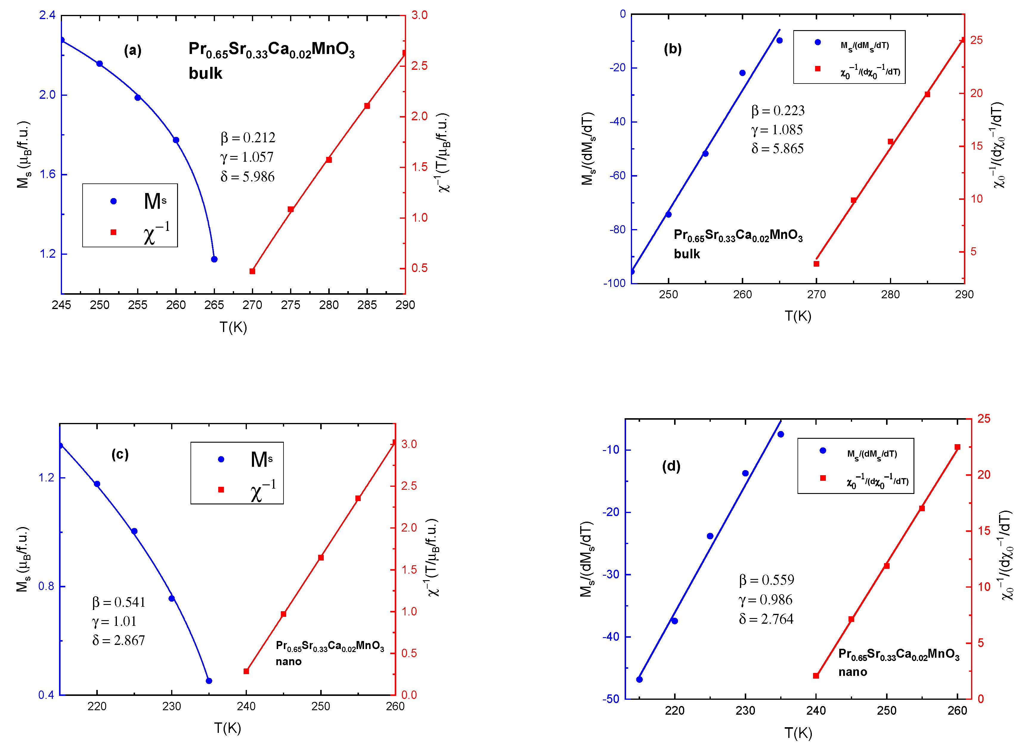
| Compound | γ | β | δ | TC (K) | |
|---|---|---|---|---|---|
| x = 0.02 | bulk | 1.057 | 0.212 | 5.986 | 273 |
| x = 0.05 | bulk | 0.981 | 0.232 | 5.228 | 261 |
| x = 0.1 | bulk | 0.985 | 0.25 | 4.94 | 244 |
| x = 0.2 | bulk | 1.036 | 0.217 | 5.774 | 201 |
| x = 0.3 | bulk | - | - | - | - |
| x = 0 | nano | 1.023 | 0.552 | 2.853 | 257 |
| x= 0.02 | nano | 1.01 | 0.541 | 2.867 | 252 |
| x = 0.05 | nano | 0.986 | 0.508 | 2.941 | 249 |
| x = 0.1 | nano | 0.977 | 0.512 | 2.908 | 239 |
| x = 0.2 | nano | 0.967 | 0.531 | 2.821 | 191 |
| x = 0.3 | nano | - | - | - | - |
| Mean field model | 1 | 0.5 | 3 | ||
| 3D Heisenberg model | 1.366 | 0.355 | 4.8 | ||
| Ising model | 1.24 | 0.325 | 4.82 | ||
| Tricritical mean field model | 1 | 0.25 | 5 | ||
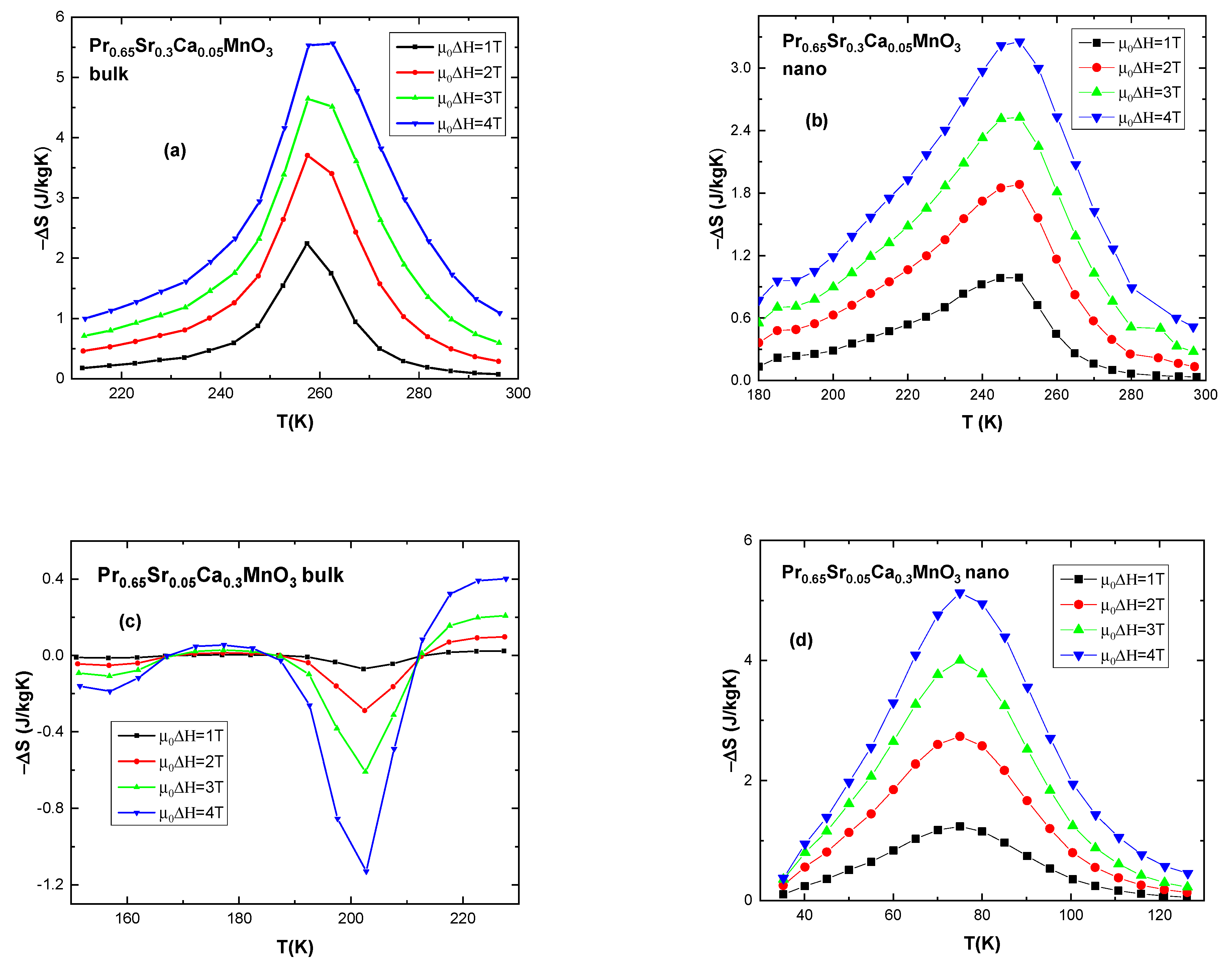
| Compound (Bulk) | TC (K) | Ms (μB/f.u.) | Hci (Oe) | |ΔSM| (J/kgK) μ0ΔH = 1 T | |ΔSM| (J/kgK) μ0ΔH = 4 T | RCP (S) (J/kg) μ0ΔH = 1 T | RCP (S) (J/kg) μ0ΔH = 4 T | Refs. |
|---|---|---|---|---|---|---|---|---|
| Pr0.65Sr0.35MnO3 | 295 | 2.3 | [12] | |||||
| Pr0.65Sr0.33Ca0.02MnO3 | 273 | 3.71 | 180 | 2.04 | 5.53 | 34 | 166 | This work |
| Pr0.65Sr0.3Ca0.05MnO3 | 261 | 3.78 | 170 | 2.24 | 5.56 | 44 | 167 | This work |
| Pr0.65Sr0.25Ca0.1MnO3 | 244 | 3.94 | 190 | 3.03 | 6.91 | 45 | 186 | This work |
| Pr0.65Sr0.15Ca0.2MnO3 | 201 | 3.97 | 160 | 4.48 | 9.21 | 60 | 270 | This work |
| Pr0.65Sr0.05Ca0.3MnO3 | 3.81 | 170 | 4.6 (40 K) | 15.3 (40 K) | 92 (40 K) | 380 (40 K) | This work | |
| La0.7Ca0.3MnO3 | 256 | 1.38 | 41 | [10] | ||||
| La0.7Sr0.3MnO3 | 365 | - | 4.44 (5 T) | 128 (5 T) | [10] | |||
| La0.6Nd0.1Ca0.3MnO3 | 233 | 1.95 | 37 | [10] | ||||
| Gd5Si2Ge2 | 276 | - | 18 (5 T) | - | 535 (5 T) | [10] | ||
| Gd | 293 | 2.8 | 35 | [10] |
| Compound (Nano) | Tc (K) | Ms (μB/f.u.) | Hci (Oe) | |ΔSM| (J/kgK) μ0ΔH = 1 T | |ΔSM| (J/kgK) μ0ΔH = 4 T | RCP(S) (J/kg) μ0ΔH = 1 T | RCP(S) (J/kg) μ0ΔH = 4 T | Refs. |
|---|---|---|---|---|---|---|---|---|
| Pr0.65Sr0.35MnO3 | 257 | 3.6 | 810 | 1.62 | 4.55 | 54 | 263 | This work |
| Pr0.65Sr0.33Ca0.02MnO3 | 252 | 3.08 | 720 | 0.69 | 2.5 | 38 | 175 | This work |
| Pr0.65Sr0.3Ca0.05MnO3 | 249 | 3.16 | 540 | 0.99 | 3.25 | 48 | 178 | This work |
| Pr0.65Sr0.25Ca0.1MnO3 | 239 | 3.49 | 510 | 1.41 | 4.37 | 39 | 215 | This work |
| Pr0.65Sr0.15Ca0.2MnO3 | 191 | 3.39 | 620 | 1.08 | 3.9 | 41 | 185 | This work |
| Pr0.65Sr0.05Ca0.3MnO3 | - | 600 | 1.23(75 K) | 5.12(75 K) | 48(75 K) | 204(75 K) | This work | |
| La0.67Ca0.33MnO3 | 260 | 0.97 (5 T) | 27 (5 T) | [63] | ||||
| Pr0.65(Ca0.6Sr0.4)0.35MnO3 | 220 | 0.75 | 21.8 | [64] | ||||
| La0.6Sr0.4MnO3 | 365 | 1.5 | 66 | [17] |
Disclaimer/Publisher’s Note: The statements, opinions and data contained in all publications are solely those of the individual author(s) and contributor(s) and not of MDPI and/or the editor(s). MDPI and/or the editor(s) disclaim responsibility for any injury to people or property resulting from any ideas, methods, instructions or products referred to in the content. |
© 2023 by the authors. Licensee MDPI, Basel, Switzerland. This article is an open access article distributed under the terms and conditions of the Creative Commons Attribution (CC BY) license (https://creativecommons.org/licenses/by/4.0/).
Share and Cite
Atanasov, R.; Ailenei, D.; Bortnic, R.; Hirian, R.; Souca, G.; Szatmari, A.; Barbu-Tudoran, L.; Deac, I.G. Magnetic Properties and Magnetocaloric Effect of Polycrystalline and Nano-Manganites Pr0.65Sr(0.35−x)CaxMnO3 (x ≤ 0.3). Nanomaterials 2023, 13, 1373. https://doi.org/10.3390/nano13081373
Atanasov R, Ailenei D, Bortnic R, Hirian R, Souca G, Szatmari A, Barbu-Tudoran L, Deac IG. Magnetic Properties and Magnetocaloric Effect of Polycrystalline and Nano-Manganites Pr0.65Sr(0.35−x)CaxMnO3 (x ≤ 0.3). Nanomaterials. 2023; 13(8):1373. https://doi.org/10.3390/nano13081373
Chicago/Turabian StyleAtanasov, Roman, Dorin Ailenei, Rares Bortnic, Razvan Hirian, Gabriela Souca, Adam Szatmari, Lucian Barbu-Tudoran, and Iosif Grigore Deac. 2023. "Magnetic Properties and Magnetocaloric Effect of Polycrystalline and Nano-Manganites Pr0.65Sr(0.35−x)CaxMnO3 (x ≤ 0.3)" Nanomaterials 13, no. 8: 1373. https://doi.org/10.3390/nano13081373