
Numerical Simulation of a Time-Dependent Electroviscous and Hybrid Nanofluid with Darcy-Forchheimer Effect between Squeezing Plates


 ,
,  and
and
Abstract
:1. Introduction
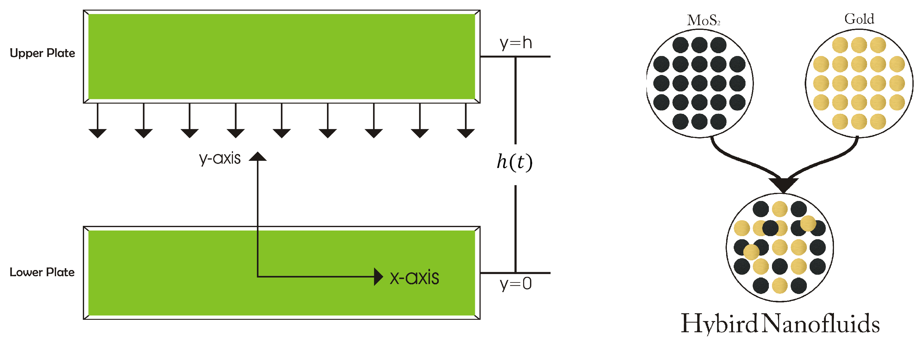
2. Formulation
3. Numerical Solution by PCM
- First order of ODEWe use the variables below to transform the PDEs given in (11)–(16) into the first order of ODEs.
- Introducing parameter q gives ODEs in the q-parameter group
- Differentiation by q reaches the following system with respect to the sensitivities of the parameter-q
- Cauchy Problemwhere and are the vector functions. By resolving the two types of Cauchy problems for each component, the system of the ODEs are satisfied automatically.and we have the boundary conditions.
- Use of Numerical SolutionAn absolute scheme has been considered for the resolution of the problem
- Take the corresponding coefficientsAs mentioned, the boundaries are commonly used for , where ; for the solution of the ODEs, we used the equation , and its corresponding matrix representation as given below.where
4. Results and Discussion
5. Concluding Remarks
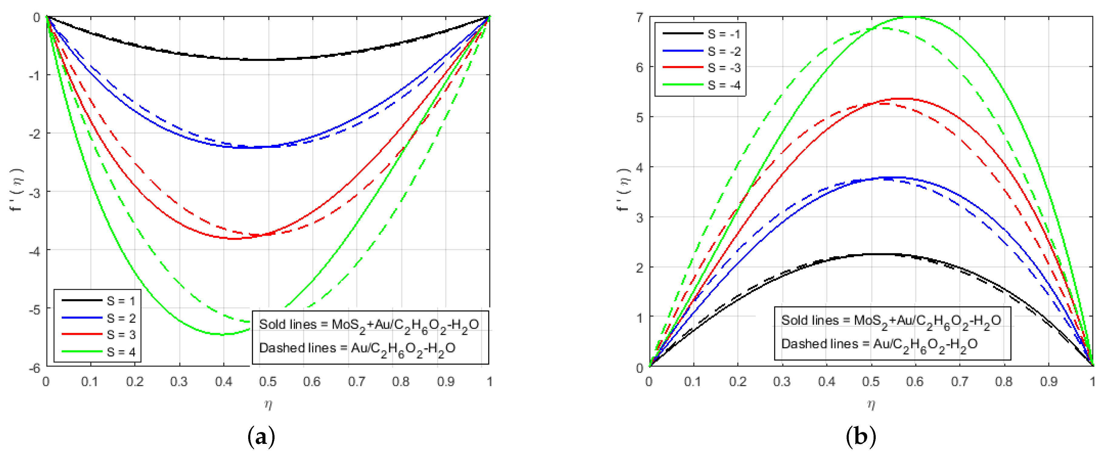
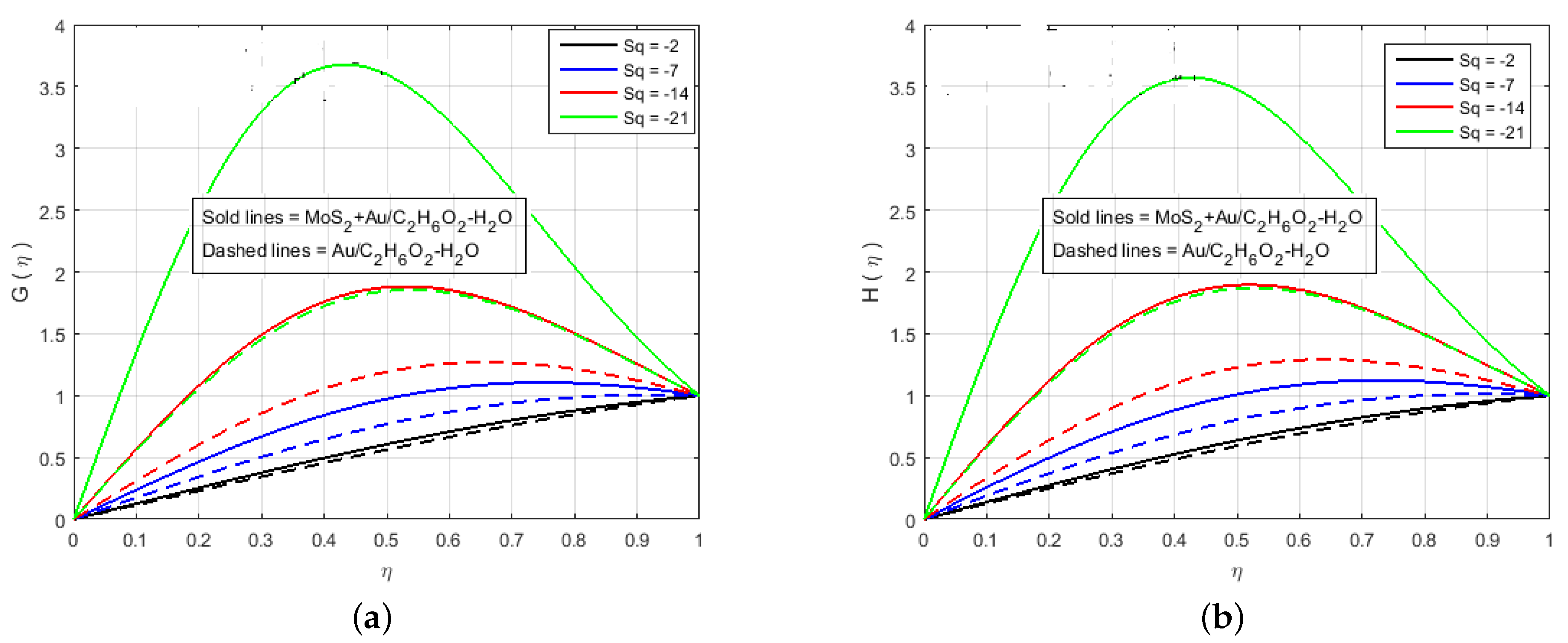
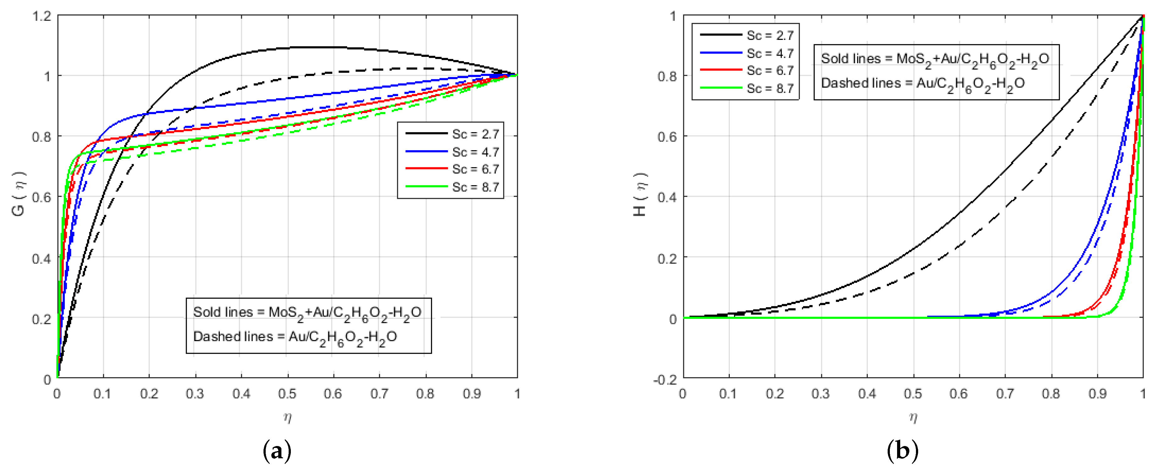
- The velocity profile shows gradually opposite behavior as a result of the augmenting value of the suction/injection parameter S.
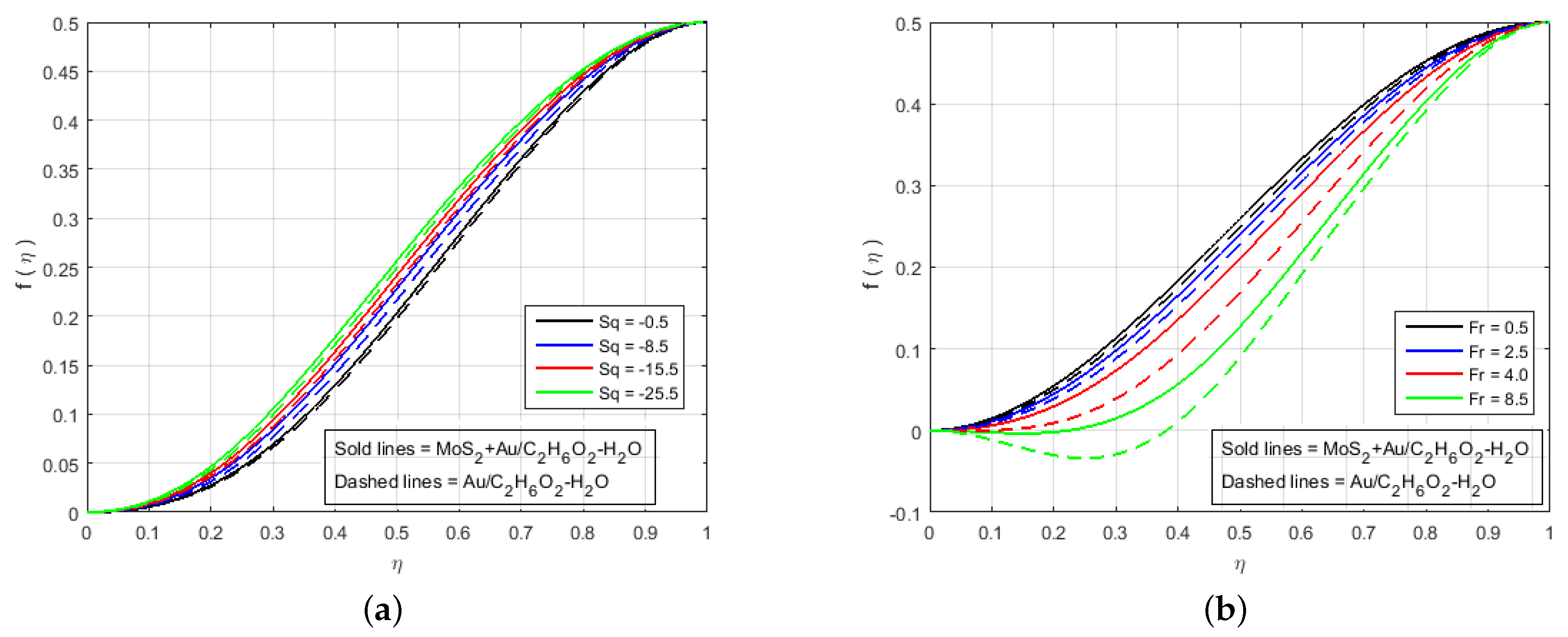
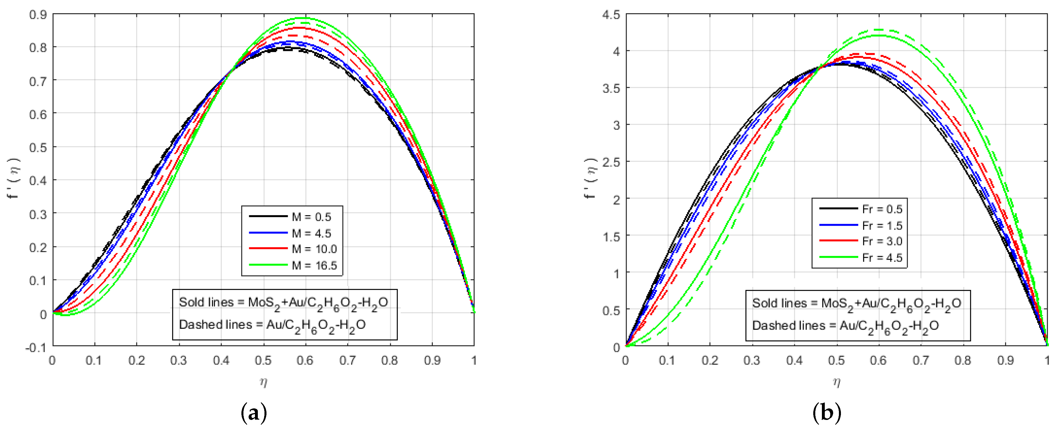
- The increment in nanomaterial volume fraction reflects the same rising influence at the velocity profile for the value of M and Sq.
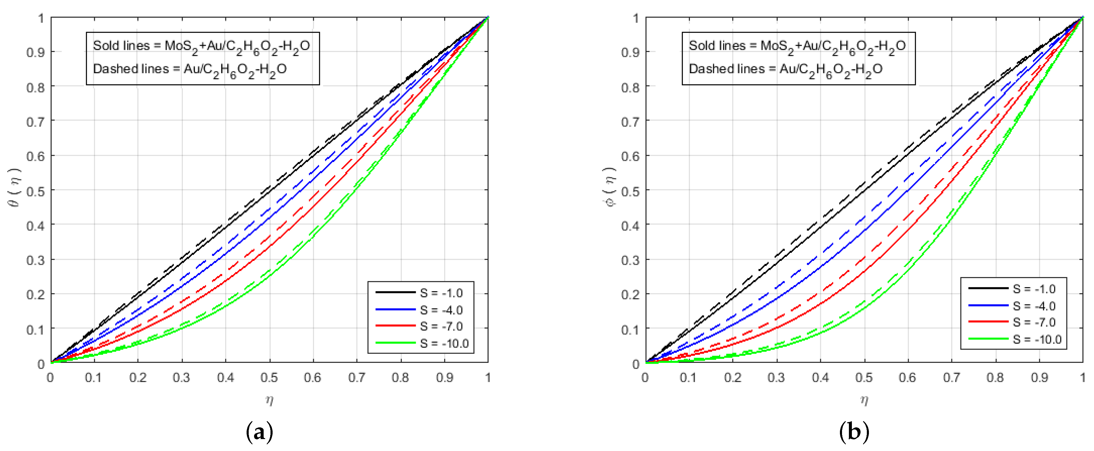
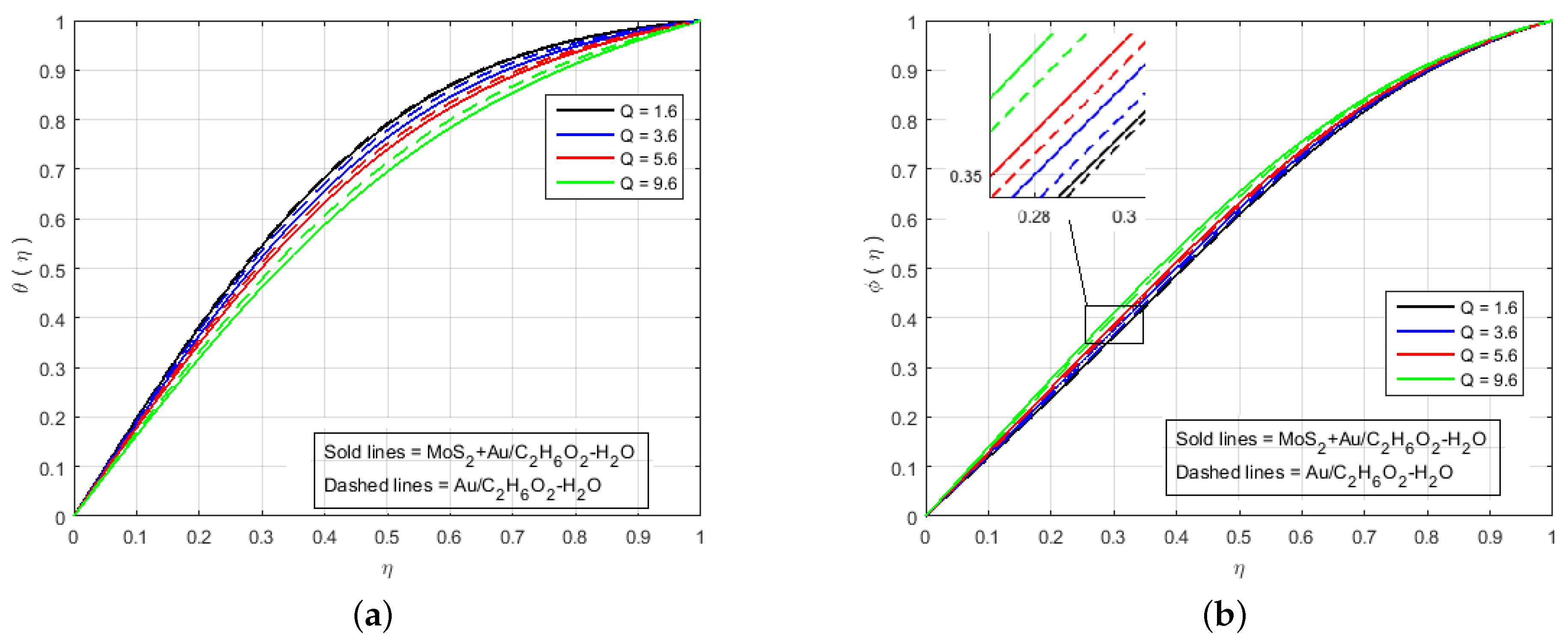
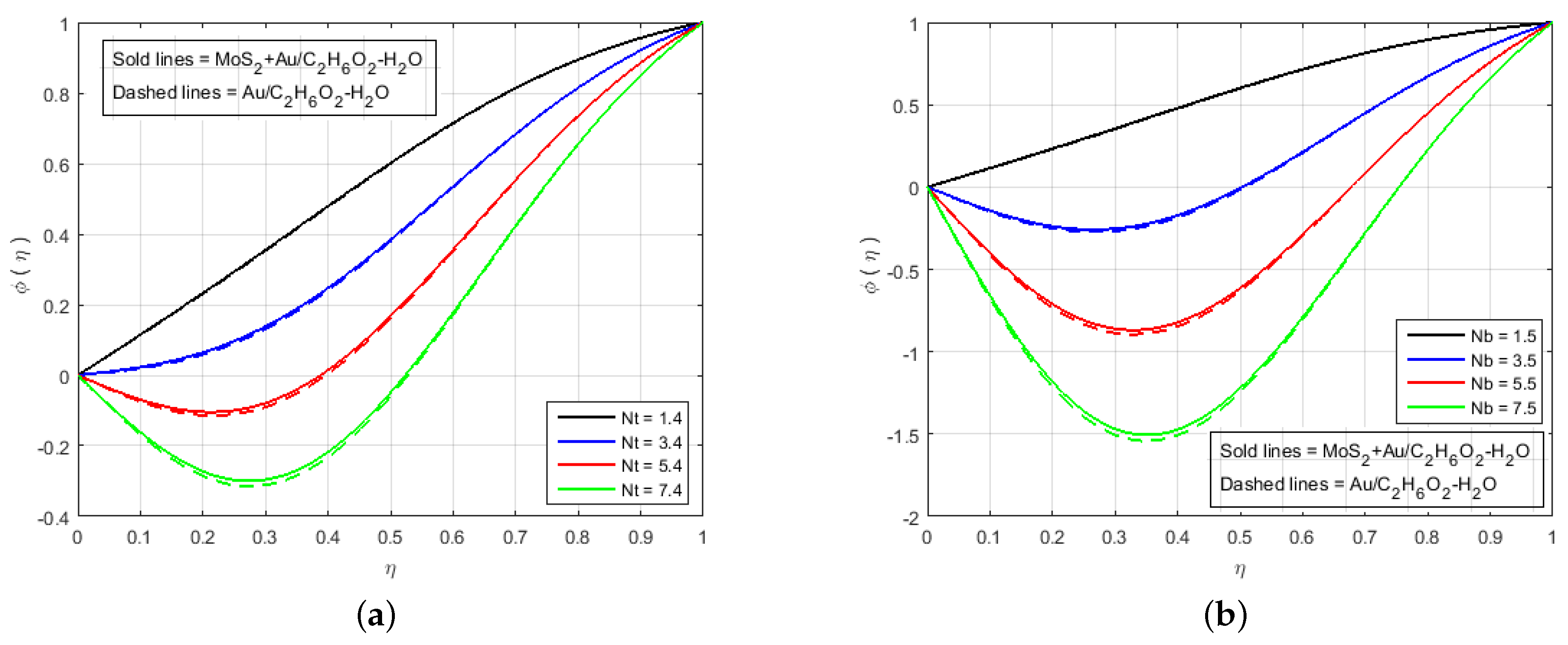
- The temperature profile and concentration profile declines with rising absolute values of nanomaterial volume fraction for .
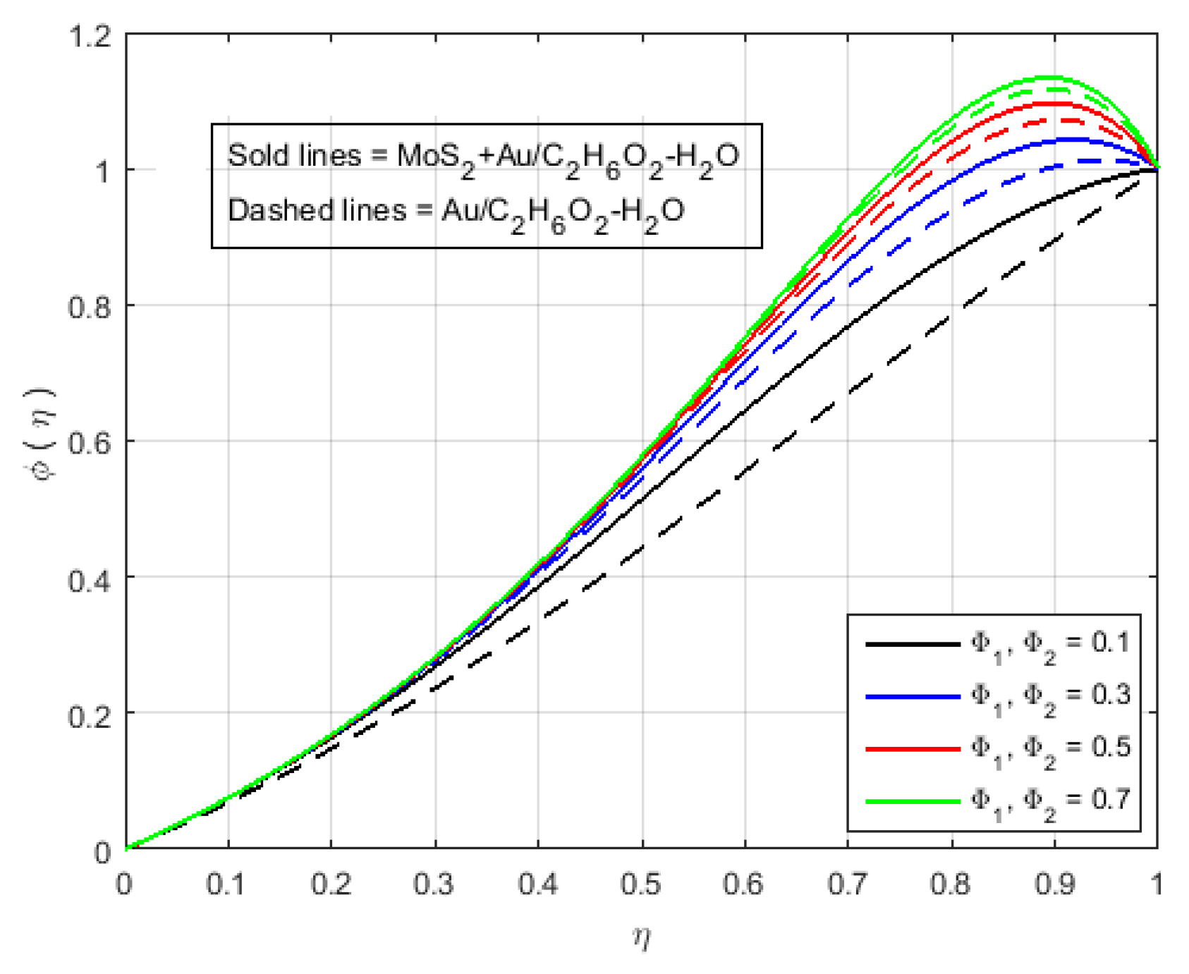
- With increasing values of nanomaterial volume fraction, the concentration profile rises.
- The higher the M and S values, the less skin friction there is at the wall.
- Skin friction is lower in the nanoparticles than in other ethylene glycol + water-based nanomaterials. Otherwise, heats the surface more efficiently than the rest of the mixtures.
Author Contributions
Funding
Institutional Review Board Statement
Informed Consent Statement
Data Availability Statement
Acknowledgments
Conflicts of Interest
References
- Choi, S.U.S.; Eastman, J.A. Enhancing thermal conductivity of fluids with nanoparticles. In Proceedings of the ASME International Mechanical Engineering Congr Expo, ASME, FED231/MD66, San Francisco, CA, USA, 12–17 November 1995; pp. 99–105. [Google Scholar]
- Eastman, J.A.; Choi, S.U.S.; Li, S.; Yu, W.; Thompson, L.J. Anomalously increased effective thermal conductivities of ethylene glycol-based nanofluids containing copper nanoparticles. Appl. Phys. Lett. 2001, 78, 718–720. [Google Scholar] [CrossRef]
- Noor, N.A.M.; Shafie, S.; Admon, M.A. Effects of Viscous Dissipation and Chemical Reaction on MHD Squeezing Flow of Casson Nanofluid between Parallel Plates in a Porous Medium with Slip Boundary Condition. Eur. Phys. J. Plus. 2020, 135, 855. [Google Scholar] [CrossRef]
- Wong, K.V.; De Leon, O. Applications of nanofluids: Current and future. Adv. Mech. Eng. 2010, 4, 519659. [Google Scholar] [CrossRef] [Green Version]
- Buongiorno, J. Convective Transport in Nanofluids. ASME J. Heat Transf. 2006, 128, 240–250. [Google Scholar] [CrossRef]
- Stefan, M. Experiments on apparent adhesion. Lond. Edinb. Dublin Philos. Mag. J. Sci. 1874, 47, 465–466. [Google Scholar] [CrossRef]
- Archibald, F.R. Load capacity and time relations for squeeze films. Trans. ASME 1956, 78, 231–245. [Google Scholar] [CrossRef]
- Reynolds, O. On the theory of lubrication and its application to Mr. Beauchamp towers experiments, including an experimental determination of the viscosity of olive oil. Philos. Trans. R. Soc. Lond. 1886, 177, 157–234. [Google Scholar] [CrossRef]
- Jackson, J.D. A study of squeezing flow. Appl. Sci. Res. 1963, 11, 148–152. [Google Scholar] [CrossRef]
- Ishizawa, S. The unsteady flow between two parallel discs with arbitary varying gap width. Bull. Jpn. Soc. Mech. Eng. 1966, 9, 533–550. [Google Scholar] [CrossRef]
- Noor, N.A.M.; Shafie, S.; Admon, M.A. Unsteady MHD squeezing flow of Jeffrey fluid in a porous medium with thermal radiation, heat generation/absorption and chemical reaction. Phys. Scr. 2020, 95, 105213. [Google Scholar] [CrossRef]
- Mabood, F.; Abdel-Rahman, R.G.; Lorenzini, G. Numerical Study of Unsteady Jeffery Fluid Flow with Magnetic Field Effect and Variable Fluid Properties. J. Therm. Sci. Eng. Appl. 2016, 8, 041003. [Google Scholar] [CrossRef]
- Ali, A.; Asghar, S. Analytic solution for oscillatory flow in a channel for Jeffrey fluid. J. Aerosp. Eng. 2012, 27, 644–651. [Google Scholar] [CrossRef]
- Akbar, N.S.; Nadeem, S.; Ali, M. Jeffrey fluid model for blood flow through a tapered artery with a stenosis. J. Mech. Med. Biol. 2011, 11, 529–545. [Google Scholar] [CrossRef]
- D’Emili, E.; Giuliani, L.; Lisi, A.; Ledda, M.; Grimaldi, S.; Montagnier, L.; Libof, A.R. Lorentz force in water: Evidence that hydronium cyclotron resonance enhances polymorphism. Electromagn. Biol. Med. 2014, 34, 370–375. [Google Scholar] [CrossRef] [PubMed]
- Sulochana, C.; Samrat, S.P. Unsteady MHD radiative flow of a nanoliquid past a permeable stretching sheet: An analytical study. J. Nanofluids 2017, 6, 711–719. [Google Scholar] [CrossRef]
- Noor, N.A.M.; Shafie, S.; Admon, M.A. Impacts of chemical reaction on squeeze flow of MHD Jeffrey fluid in horizontal porous channel with slip condition. Phys. Scr. 2021, 96, 035216. [Google Scholar] [CrossRef]
- Nallapu, S.; Radhakrishnamacharya, G. Jeffrey fluid flow through porous medium in the presence of magnetic field in narrow tubes. Int. J. Eng. Math. 2014, 2014, 713831. [Google Scholar] [CrossRef] [Green Version]
- Ahmad, K.; Ishak, A. Magnetohydrodynamic flow and heat transfer of a Jeffrey fluid towards a stretching vertical surface. Therm. Sci. 2015, 2015, 29. [Google Scholar] [CrossRef] [Green Version]
- Hu, L.; Harrison, J.D.; Masliyah, J.H. Numerical Model of Electrokinetic Flow for Capillary Electrophoresis. J. Colloid Interface Sci. 1999, 215, 300–312. [Google Scholar] [CrossRef]
- Culbertson, C.; Ramsey, R.; Ramsey, J.M. Electroosmotically induced hydraulic pumping on microchips: Differential ion transport. Anal. Chem. 2000, 72, 2285–2291. [Google Scholar] [CrossRef]
- Yang, C.; Li, D.; Masliyah, J.H. Modeling forced liquid convection in rectangular microchannels with electrokinetic effects. Int. J. Heat Mass Transf. 1998, 41, 4229–4249. [Google Scholar] [CrossRef]
- Arulanandam, S.; Li, D. Liquid transport in rectangular microchannels by electroosmotic pumping. Colloids Surf. A Physicochem. Eng. Asp. 2000, 161, 89–102. [Google Scholar] [CrossRef]
- Whitesides, G.; Stroock, A. Flexible methods for microfluidics. Phys. Fluids 2001, 54, 42–48. [Google Scholar] [CrossRef] [Green Version]
- Gad-El-Hak, M. (Ed.) The MEMS Handbook, 2nd ed.; CRC Press: Boca Raton, FL, USA, 2006. [Google Scholar]
- Stone, H.A.; Kim, S. Microfluidics: Basic issues, applications, and challenges. AIChE J. 2001, 47, 1250–1254. [Google Scholar] [CrossRef]
- Stone, H.A.; Stroock, A.D.; Ajdari, A. Engineering flows in small devices: Microfluidics towards a lab-on-a-chip. Annu. Rev. Fluid Mech. 2004, 36, 381–411. [Google Scholar] [CrossRef] [Green Version]
- Khashi’ie, N.S.; Waini, I.; Arifin, N.M.; Pop, I. Unsteady squeezing flow of Cu-Al2O3/water hybrid nanofluid in a horizontal channel with magnetic field. Sci. Rep. 2021, 11, 14128. [Google Scholar] [CrossRef] [PubMed]
- Khan, M.S.; Rehan, A.S.; Amjad, A.; Aamir, K. Parametric investigation of the Nernst–Planck model and Maxwell–s equations for a viscous fluid between squeezing plates. Bound. Value Probl. 2019, 2019, 107. [Google Scholar] [CrossRef] [Green Version]
- Khan, M.S.; Rehan, A.S.; Aamir, K. Effect of variable magnetic field on the flow between two squeezing plates. Eur. Phys. J. Plus 2019, 134, 219. [Google Scholar] [CrossRef]
- Shah, R.A.; Anjum, M.N.; Khan, M.S. Analysis of unsteady squeezing flow between two porous plates with variable magnetic field. Int. J. Adv. Eng. Manag. Sci. 2017, 3, 239756. [Google Scholar]
- Khan, A.; Shah, R.A.; Alam, M.K.; Rehman, S.; Shahzad, M.; Almad, S.; Khan, M.S. Flow dynamics of a time-dependent non-Newtonian and non-isothermal fluid between coaxial squeezing disks. Adv. Mech. Eng. 2021, 13, 16878140211033370. [Google Scholar] [CrossRef]
- Khan, M.S.; Mei, S.; Fernandez-Gamiz, U.; Noeiaghdam, S.; Shah, S.A.; Khan, A. Numerical Analysis of Unsteady Hybrid Nanofluid Flow Comprising CNTs-Ferrousoxide/Water with Variable Magnetic Field. Nanomaterials 2022, 12, 180. [Google Scholar] [CrossRef]
- Shah, R.A.; Ullah, H.; Khan, M.S.; Khan, A. Parametric analysis of the heat transfer behavior of the nano-particle ionic-liquid flow between concentric cylinders. Adv. Mech. Eng. 2021, 13, 16878140211024009. [Google Scholar] [CrossRef]
- Sajid, T.; Jamshed, W.; Shahzad, F.; Eid, M.R.; Alshehri, H.M.; Goodarzi, M.; Nisar, K.S. Micropolar fluid past a convectively heated surface embedded with nth order chemical reaction and heat source/sink. Phys. Scr. 2021, 96, 104010. [Google Scholar] [CrossRef]
- Jamshed, W.; Goodarzi, M.; Prakash, M.; Nisar, K.S.; Zakarya, M.; Abdel-Aty, A.H. Evaluating the unsteady Casson nanofluid over a stretching sheet with solar thermal radiation: An optimal case study. Case Stud. Therm. Eng. 2021, 26, 101160. [Google Scholar] [CrossRef]
- Waqas, H.; Farooq, U.; Khan, S.A.; Alshehri, H.M.; Goodarzi, M. Numerical analysis of dual variable of conductivity in bioconvection flow of Carreau–Yasuda nanofluid containing gyrotactic motile microorganisms over a porous medium. J. Therm. Anal. Calorim. 2021, 145, 2033–2044. [Google Scholar] [CrossRef]
- Davidson, M.R.; Bharti, R.P.; Liovic, P.; Harvie, D.J. Electroviscous effects in low Reynolds number flow through a microfluidic contraction with rectangular cross-section. Proc. World Acad. Sci. Eng. Technol. 2008, 30, 256–260. [Google Scholar]
- Park, H.M.; Lee, J.S.; Kim, T.W. Comparison of the Nernst–Planck model and the Poisson–Boltzmann model for electroosmotic flows in microchannels. J. Colloid Interface Sci. 2007, 315, 731–739. [Google Scholar] [CrossRef]
- Saeed, A.; Kumam, P.; Gul, T.; Alghamdi, W.; Kumam, W.; Khan, A. Darcy–Forchheimer couple stress hybrid nanofluids flow with variable fluid properties. Sci. Rep. 2021, 11, 19612. [Google Scholar] [CrossRef]


| Physical Properties | ||||
|---|---|---|---|---|
| MoS | 5060 | |||
| Au (Gold) | 19300 | 130 | 310 | |
| 3630 |
| Present | Najiyah S.K. et al. [28] | Present | Najiyah S.K. et al. [28] | ||
| 0 | 0.5 | 4.7133540 | 4.7133028 | −7.4111453 | −7.4111525 |
| 1 | 0.5 | 4.7390482 | 4.7390165 | −7.5916641 | −7.5916177 |
| 4 | 0.5 | 4.8202618 | 4.8202511 | −8.1103709 | −8.1103342 |
| 9 | 0.5 | 4.3964712 | 4.9648698 | −8.9100425 | −8.9100956 |
| 4 | 0.0 | 1.8424315 | 1.8424469 | −4.5878710 | −4.5878911 |
| 4 | 0.3 | 3.6536010 | 3.6536948 | −6.6656598 | −6.6656620 |
| 4 | 0.6 | 5.3912487 | 5.3912475 | −8.8514001 | −8.8514442 |
| 4 | 1.0 | 7.5934008 | 7.5934262 | −11.9485561 | −11.9485843 |
| Present | Najiyah S.K. et al. [28] | |||
|---|---|---|---|---|
| 0 | 1 | 0.5 | 1.814699 | 1.814634 |
| 0.25 | 1 | 0 | −1.171512 | −1.171551 |
| 0.25 | 1 | 0.5 | 1.808145 | 1.808177 |
| 0.25 | 0 | 0.5 | 4.719601 | 4.719656 |
| 0.25 | 1.5 | 0.5 | 0.283965 | 0.283948 |
| 0.25 | 1 | 1 | 4.573012 | 4.573016 |
| 1 | 1 | 0.5 | 1.789303 | 1.789372 |
| PCM | BVP4C | HAM | PCM | BVP4C | HAM | |
|---|---|---|---|---|---|---|
| 0 | 3.0934 | 3.0931 | 3.0926 | −0.8443 | −0.8440 | −0.8438 |
| 0.1 | 3.0988 | 3.0981 | 3.0978 | −0.8615 | −0.8612 | −0.8608 |
| 0.2 | 3.1042 | 3.1038 | 3.1033 | −0.8791 | −0.8788 | −0.8783 |
| 0.3 | 3.1096 | 3.1091 | 3.1087 | −0.8969 | −0.8963 | −0.8962 |
| 0.4 | 3.1151 | 3.1145 | 3.1139 | −0.9151 | −0.9146 | −0.9140 |
| 0.5 | 3.1206 | 3.1201 | 3.1210 | −0.9336 | −0.9331 | −0.9325 |
| 0.6 | 3.1261 | 3.1255 | 3.1250 | −0.9523 | −0.9518 | −0.9511 |
| 0.7 | 3.1316 | 3.1310 | 3.1303 | −0.9714 | −0.9709 | −0.9704 |
| 0.8 | 3.1372 | 3.1365 | 3.1360 | −0.9908 | −0.9902 | −0.9914 |
| 0.9 | 3.1428 | 3.1423 | 3.1416 | −1.0105 | −1.0100 | −1.0111 |
| 1 | 3.1484 | 3.1478 | 3.1471 | −1.0306 | −1.0302 | −1.0310 |
Publisher’s Note: MDPI stays neutral with regard to jurisdictional claims in published maps and institutional affiliations. |
© 2022 by the authors. Licensee MDPI, Basel, Switzerland. This article is an open access article distributed under the terms and conditions of the Creative Commons Attribution (CC BY) license (https://creativecommons.org/licenses/by/4.0/).
Share and Cite
Khan, M.S.; Mei, S.; Shabnam; Fernandez-Gamiz, U.; Noeiaghdam, S.; Khan, A. Numerical Simulation of a Time-Dependent Electroviscous and Hybrid Nanofluid with Darcy-Forchheimer Effect between Squeezing Plates. Nanomaterials 2022, 12, 876. https://doi.org/10.3390/nano12050876
Khan MS, Mei S, Shabnam, Fernandez-Gamiz U, Noeiaghdam S, Khan A. Numerical Simulation of a Time-Dependent Electroviscous and Hybrid Nanofluid with Darcy-Forchheimer Effect between Squeezing Plates. Nanomaterials. 2022; 12(5):876. https://doi.org/10.3390/nano12050876
Chicago/Turabian StyleKhan, Muhammad Sohail, Sun Mei, Shabnam, Unai Fernandez-Gamiz, Samad Noeiaghdam, and Aamir Khan. 2022. "Numerical Simulation of a Time-Dependent Electroviscous and Hybrid Nanofluid with Darcy-Forchheimer Effect between Squeezing Plates" Nanomaterials 12, no. 5: 876. https://doi.org/10.3390/nano12050876