
Mössbauer Spectroscopy with a High Velocity Resolution in the Studies of Nanomaterials
 ,
, 


Abstract
:1. Introduction
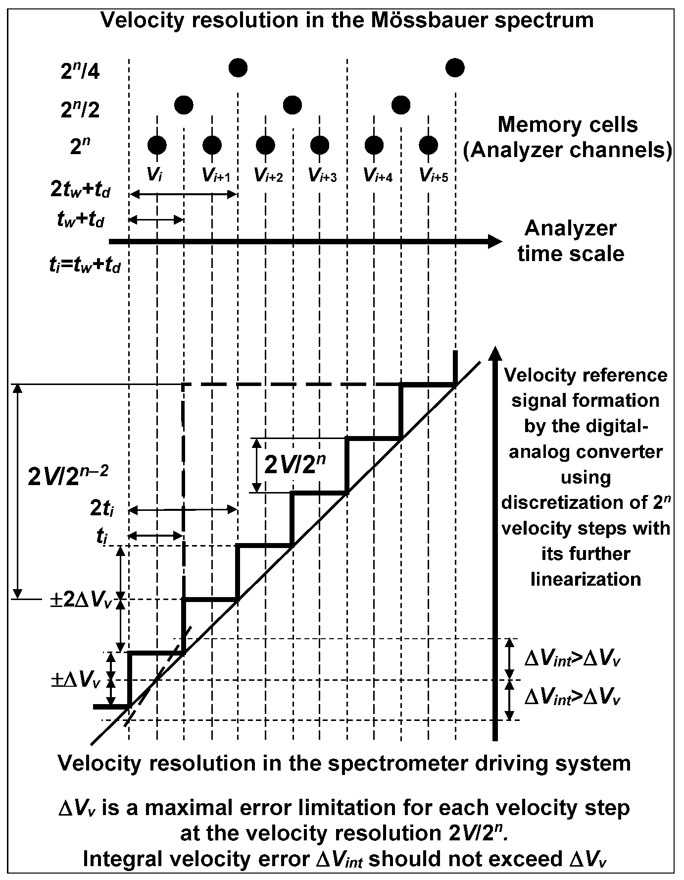
2. Mössbauer Spectroscopy with a High Velocity Resolution
3. Nanoparticles in Biology, Medicine and Pharmacy
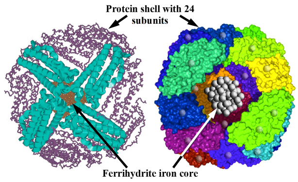
3.1. Nanosized Iron Cores in Human Liver Ferritin
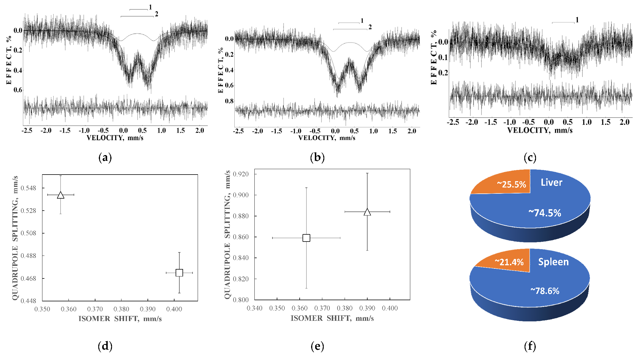
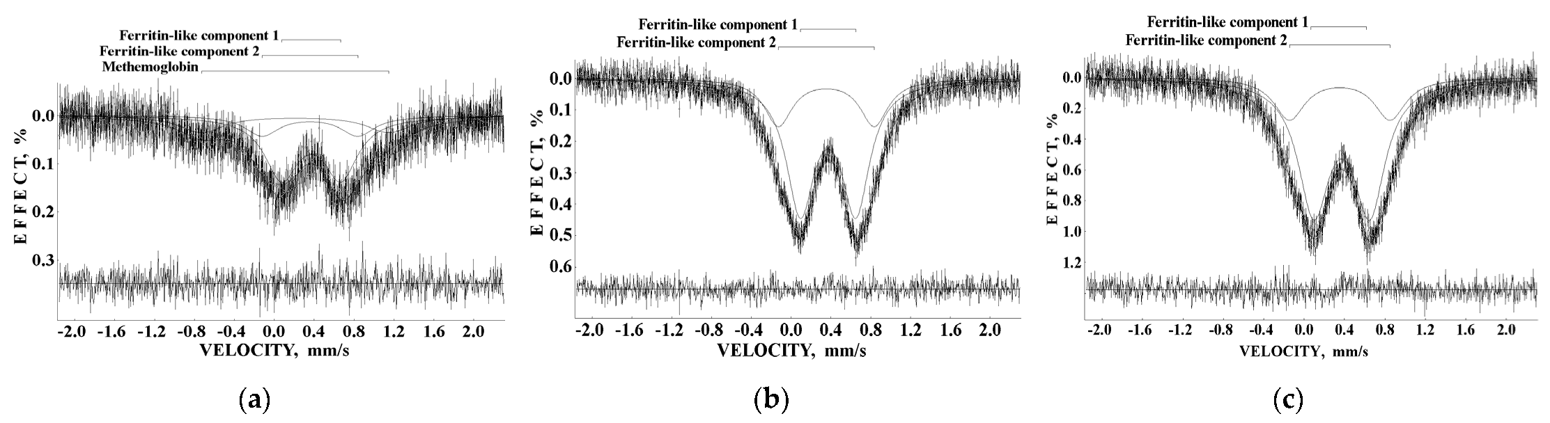
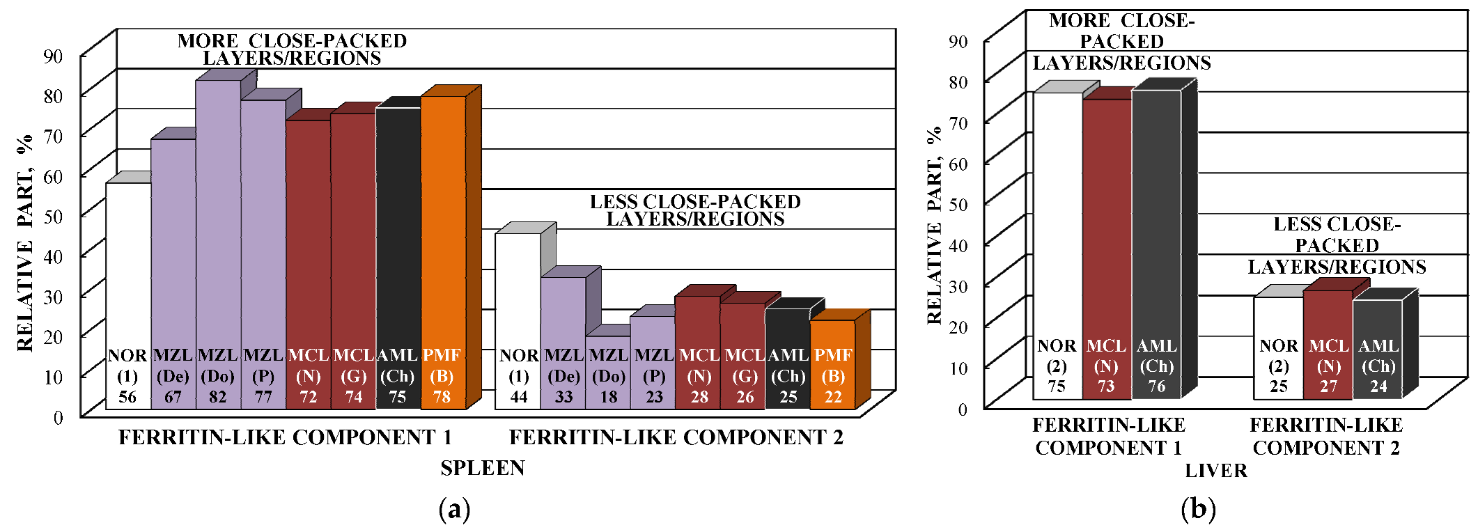
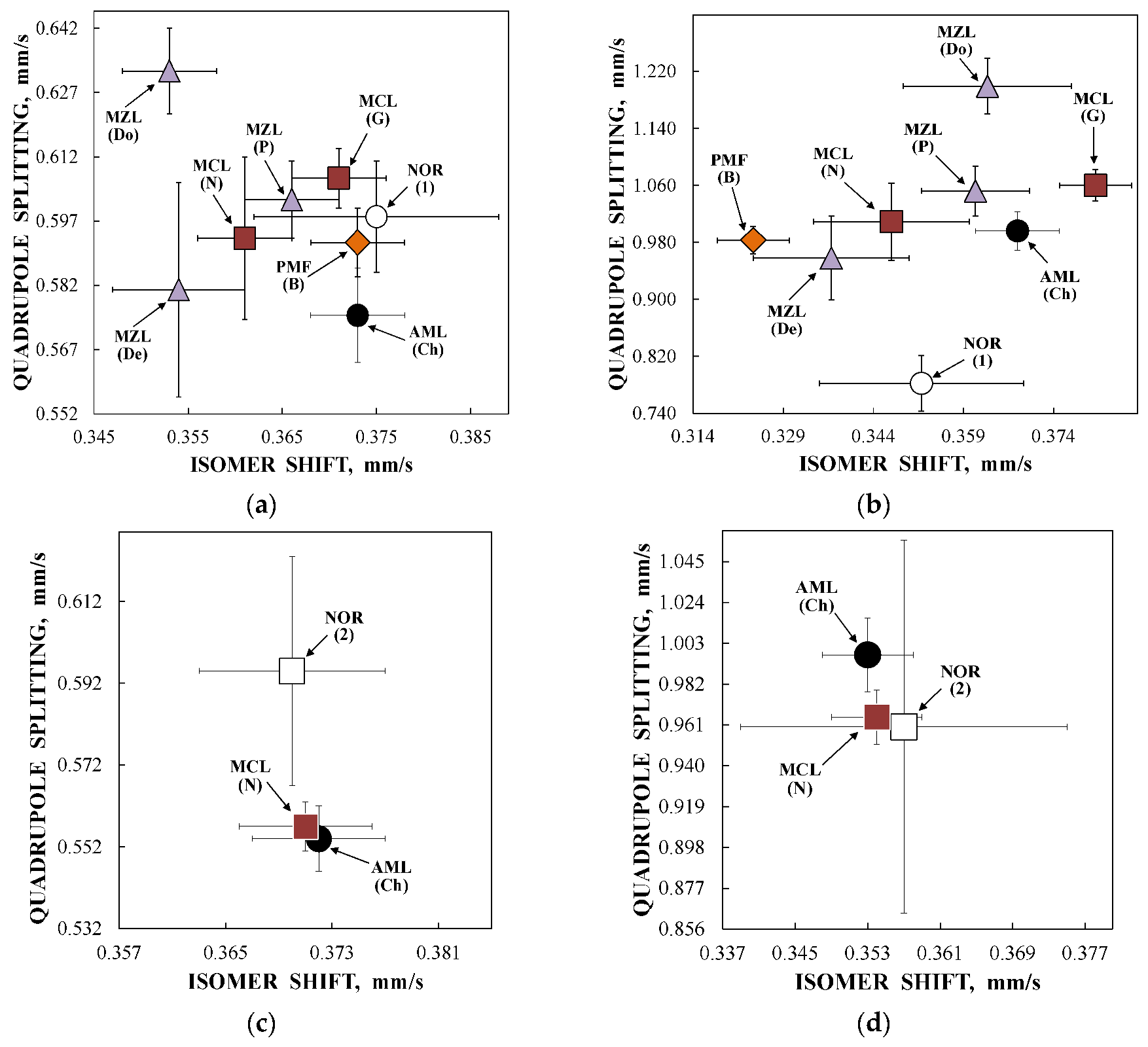
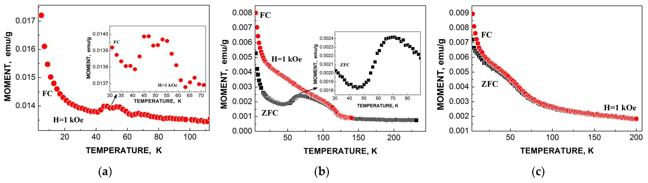
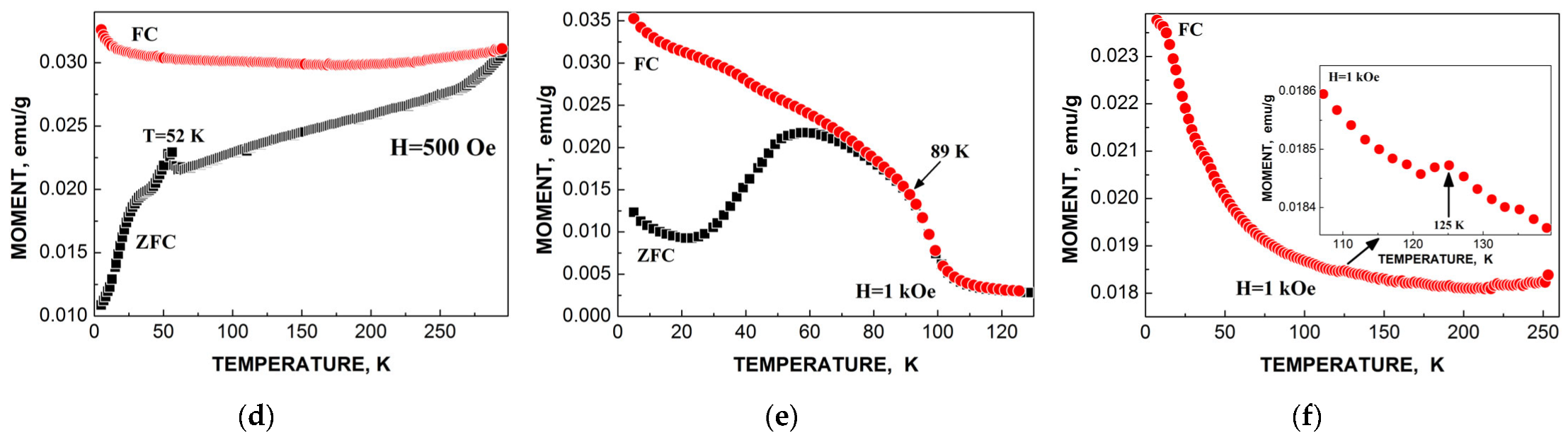
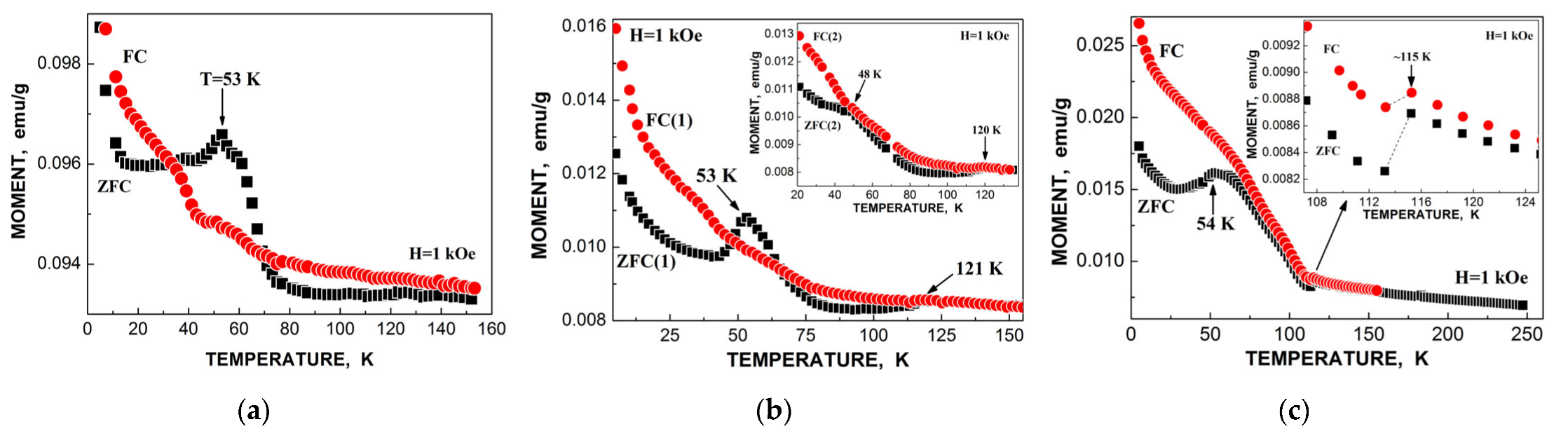
3.2. Nanosized Iron Cores in Ferritin in Liver and Spleen Tissues
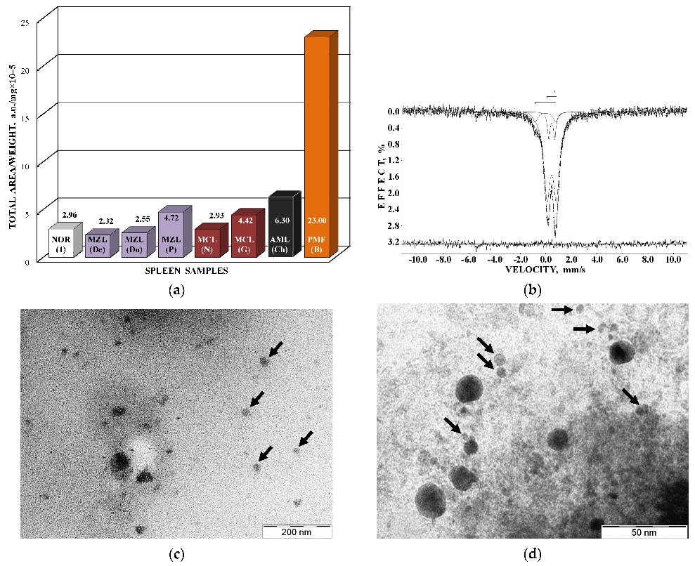
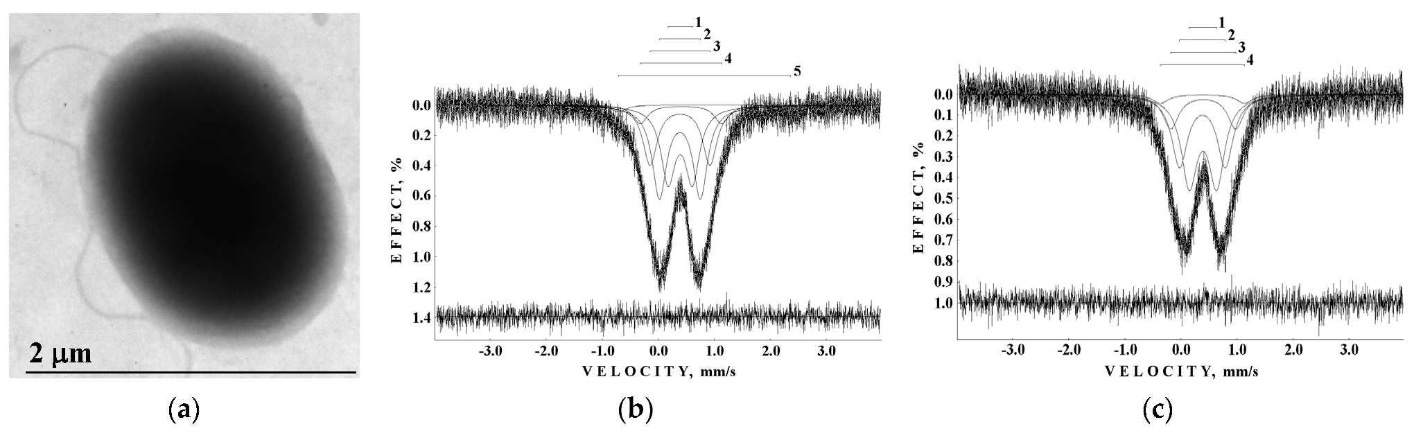
3.3. Nanosized Iron Cores in Ferritin in Bacteria
3.4. Nanosized Iron Cores in Pharmaceutical Ferritin Analogues
3.5. Nanoparticles for Magnetic Fluids and Other Medical Aims
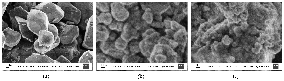
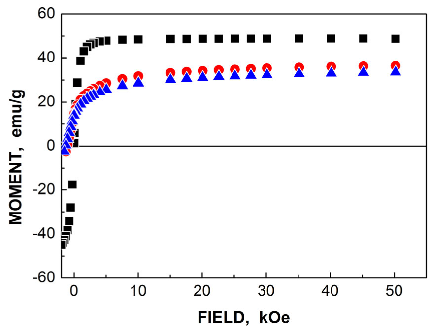
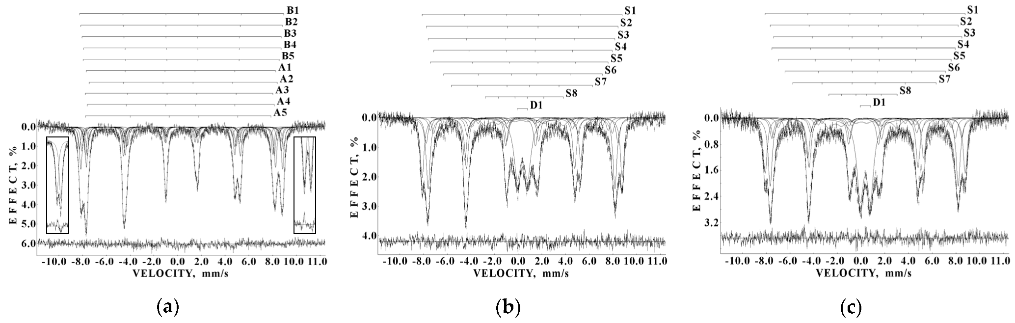
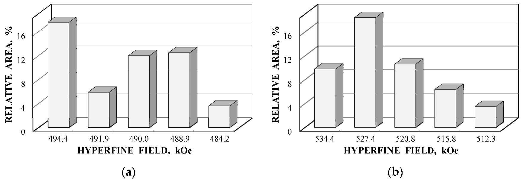
4. Nanosized Ferrites
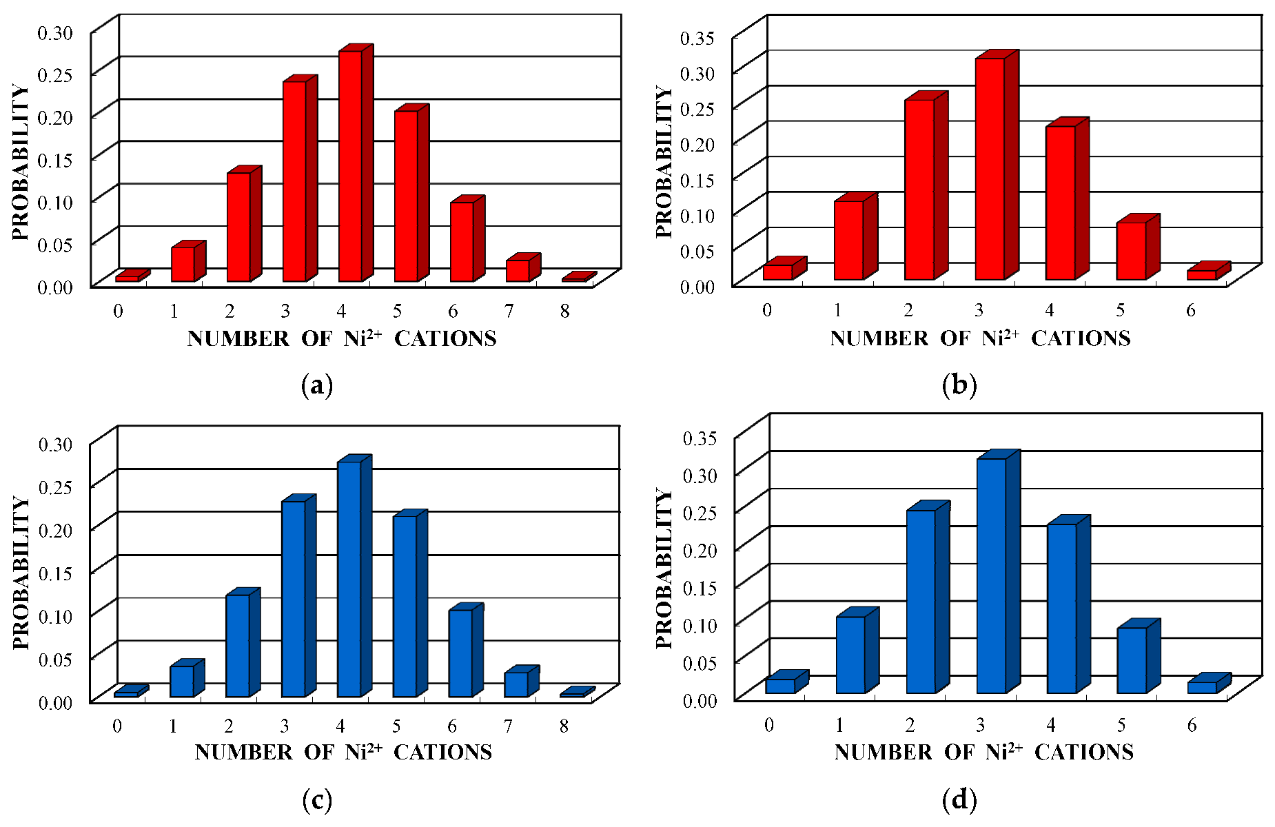
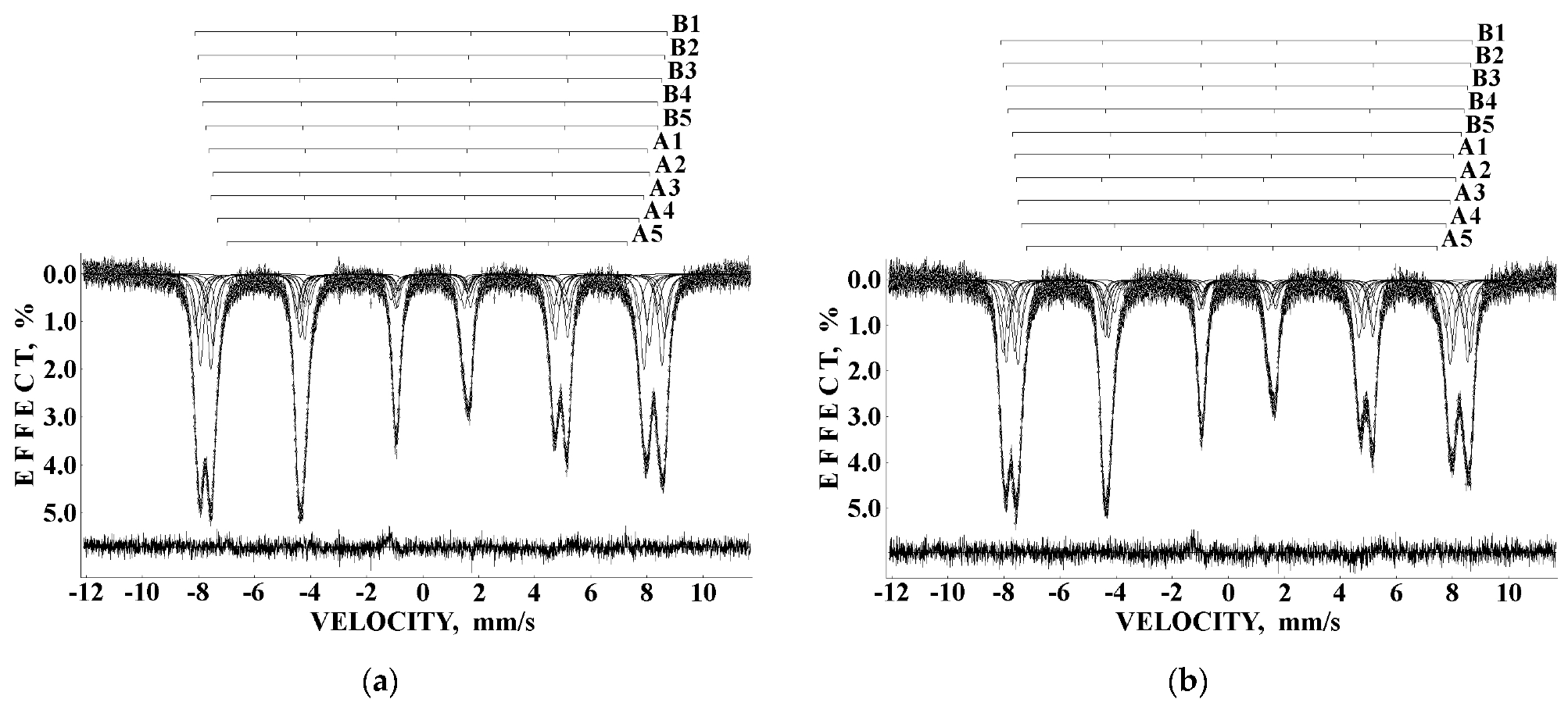
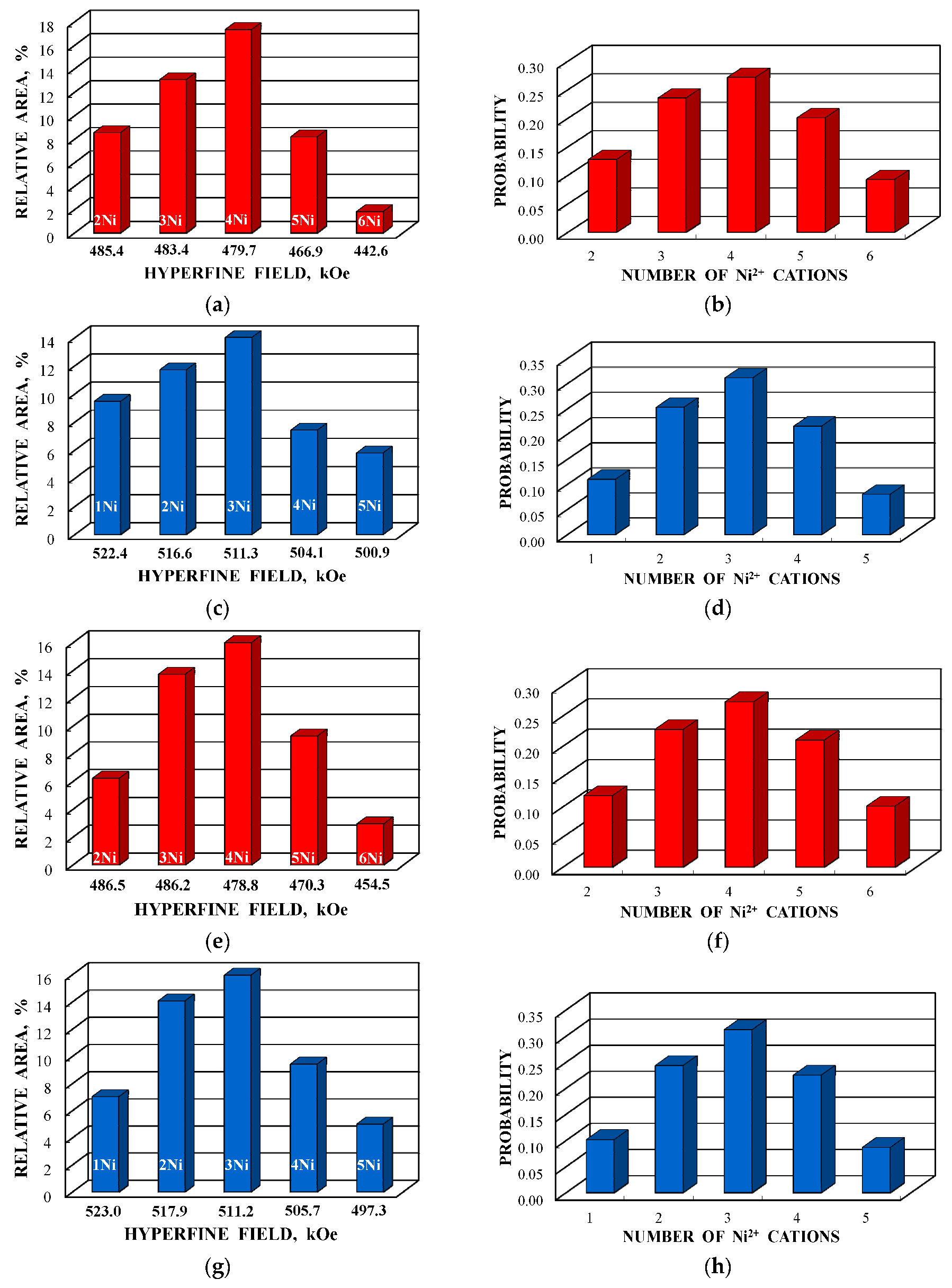
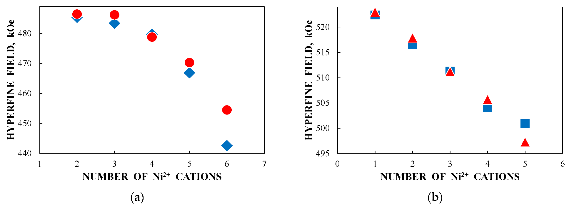
4.1. Nickel Ferrites
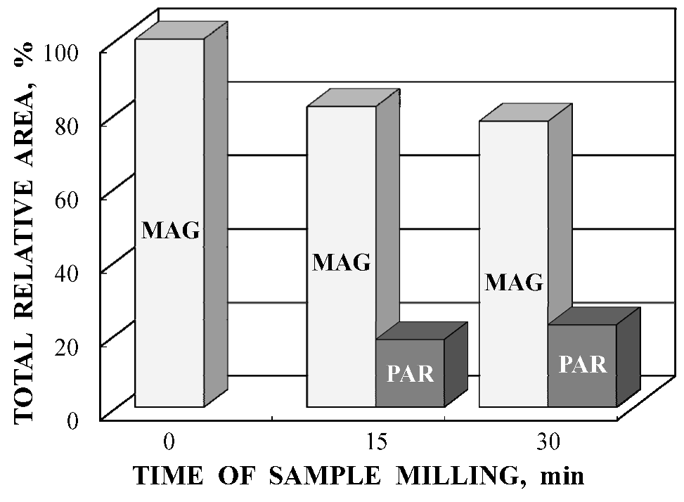
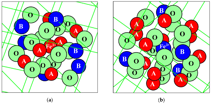
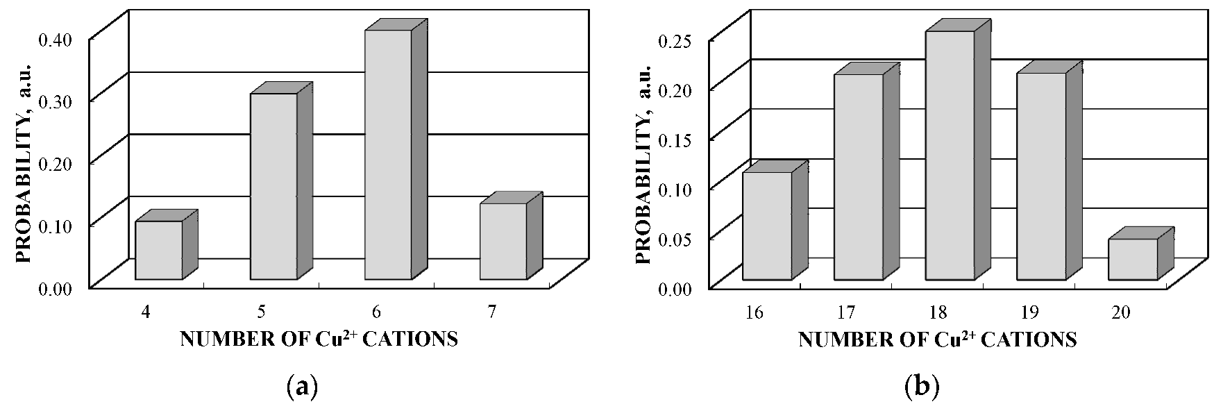
4.2. Copper Ferrites
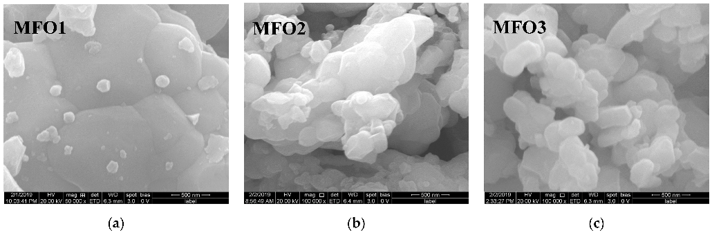
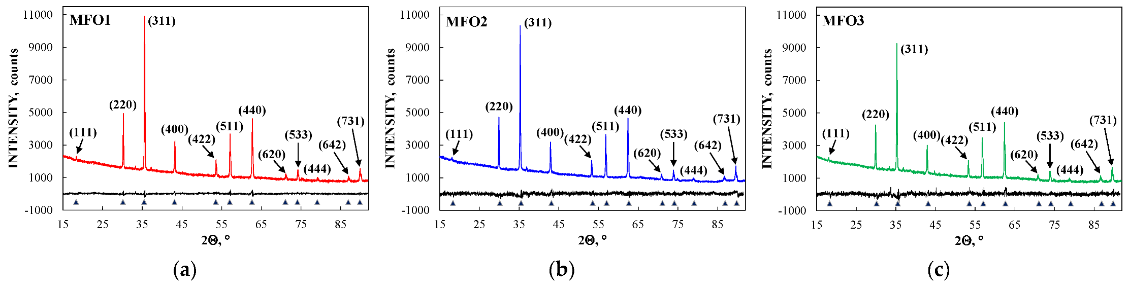
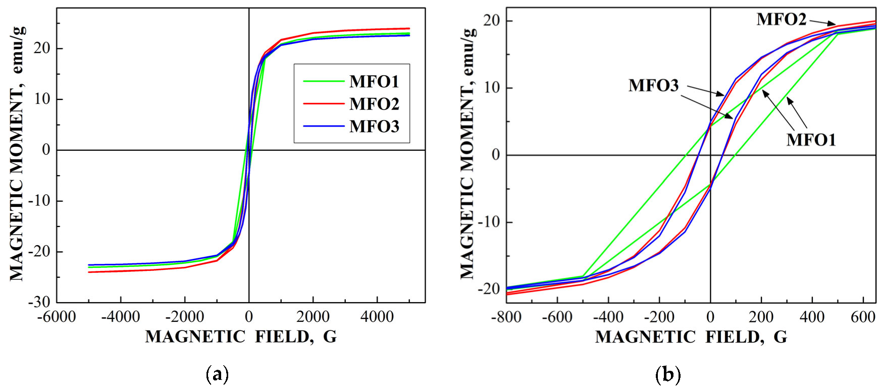
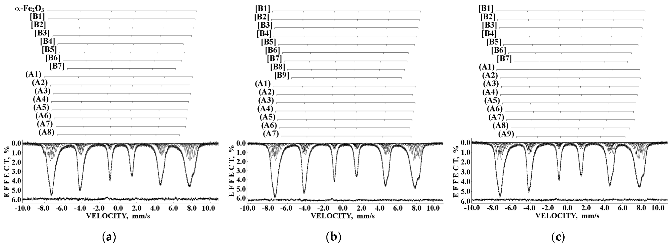
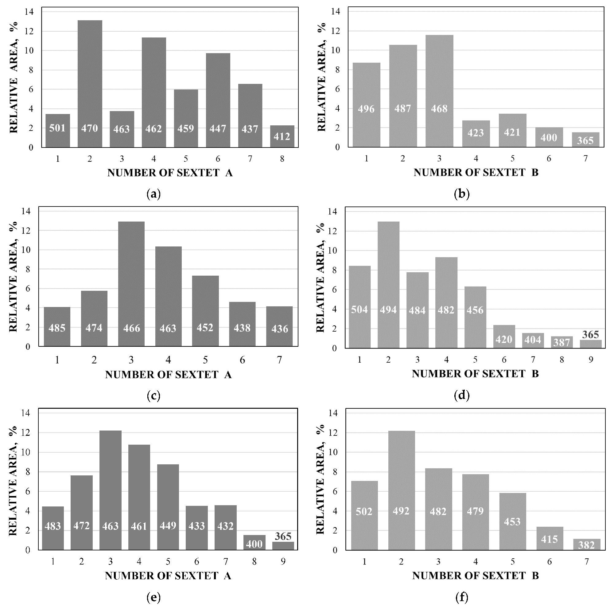
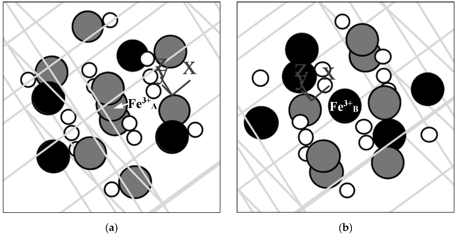
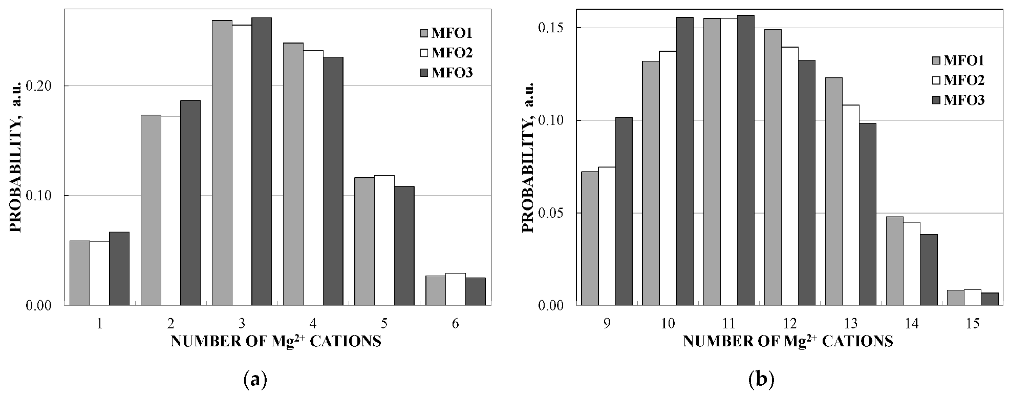
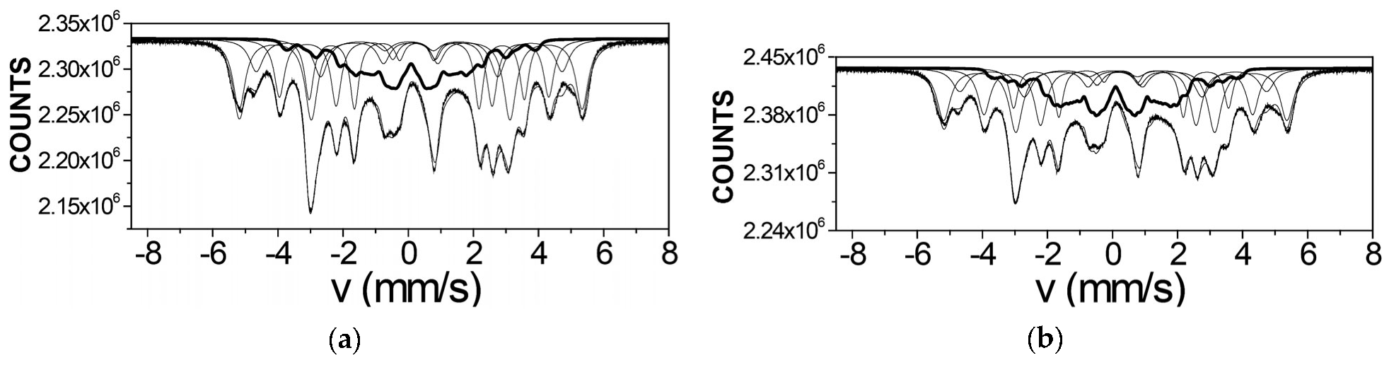
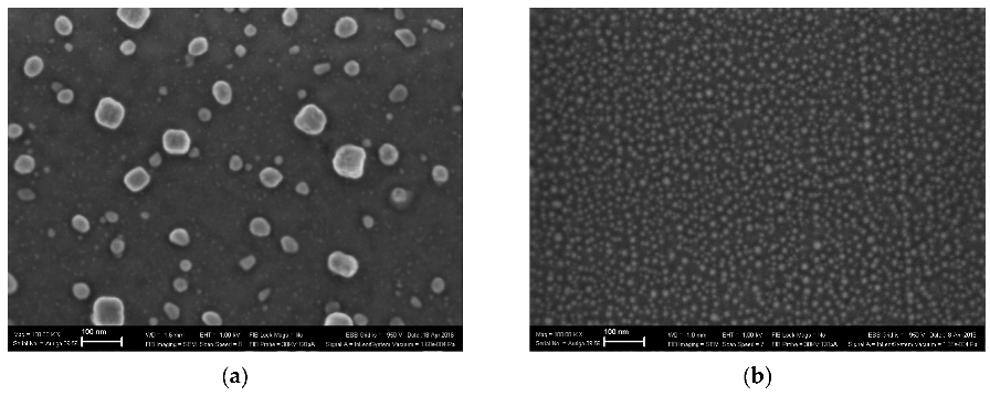
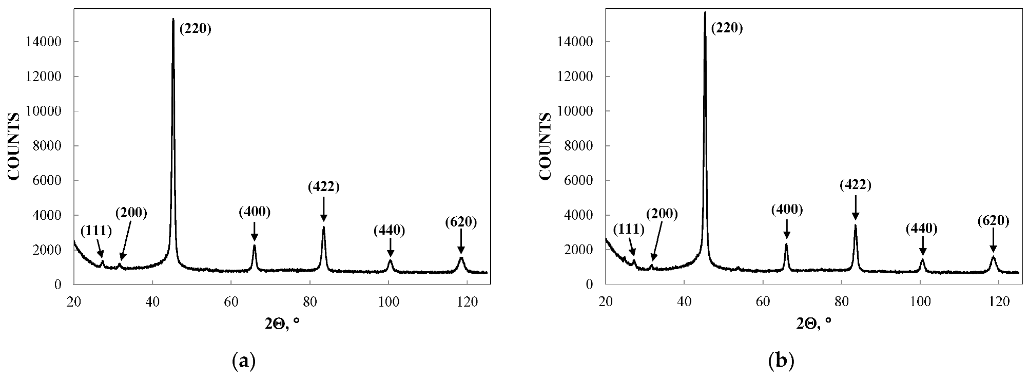
4.3. Magnesium Ferrites
5. FINEMET Alloys
6. Conclusions
Author Contributions
Funding
Institutional Review Board Statement
Informed Consent Statement
Data Availability Statement
Acknowledgments
Conflicts of Interest
References
- Bhushan, B. (Ed.) Springer Handbook of Nanotechnology, 2nd ed.; Springer Science+Business Media, Inc.: Berlin/Heidelberg, Germany; New York, NY, USA, 2007; pp. 1–1916. [Google Scholar]
- Binns, C. Introduction to Nanoscience and Nanotechnology; John Wiley & Sons, Inc.: Hoboken, NJ, USA, 2010; pp. 1–301. [Google Scholar]
- Sellmyer, D.; Skomski, R. (Eds.) Advanced Magnetic Nanostructures; Springer Science+Business Media, Inc.: Boston, MA, USA, 2006; pp. 1–508. [Google Scholar]
- Berry, C.C.; Curtis, A.S.G. Functionalisation of magnetic nanoparticles for applications in biomedicine. J. Phys. D Appl. Phys. 2003, 36, R198–R206. [Google Scholar] [CrossRef]
- Pankhurst, Q.A.; Connolly, J.; Jones, S.K.; Dobson, J. Applications of magnetic nanoparticles in biomedicine. J. Phys. D Appl. Phys. 2003, 36, R167–R181. [Google Scholar] [CrossRef] [Green Version]
- Arruebo, M.; Fernández-Pacheco, R.; Ibarra, M.R.; Santamaría, J. Magnetic nanoparticles for drug delivery. Nano Today 2007, 2, 22–32. [Google Scholar] [CrossRef]
- Pankhurst, Q.A.; Thanh, N.K.T.; Jones, S.K.; Dobson, J. Progress in applications of magnetic nanoparticles in biomedicine. J. Phys. D Appl. Phys. 2009, 42, 224001. [Google Scholar] [CrossRef] [Green Version]
- Amstad, E.; Textora, M.; Reimhult, E. Stabilization and functionalization of iron oxide nanoparticles for biomedical applications. Nanoscale 2011, 3, 2819. [Google Scholar] [CrossRef] [PubMed] [Green Version]
- Marszałł, M.P. Application of magnetic nanoparticles in pharmaceutical sciences. Pharm. Res. 2011, 28, 480–483. [Google Scholar] [CrossRef] [Green Version]
- Hasany, S.F.; Ahmed, I.; Rehman, R.J.A. Systematic review of the preparation techniques of iron oxide magnetic nanoparticles. Nanosci. Nanotech. 2012, 2, 148–158. [Google Scholar] [CrossRef] [Green Version]
- Wu, W.; Wu, Z.; Yu, T.; Jiang, C.; Kim, W.-S. Recent progress on magnetic iron oxide nanoparticles: Synthesis, surface functional strategies and biomedical applications. Sci. Technol. Adv. Mater. 2015, 16, 023501. [Google Scholar] [CrossRef]
- Hedayatnasab, Z.; Abnisa, F.; Daud, W.M.A.W. Review on magnetic nanoparticles for magnetic nanofluid hyperthermia application. Mater. Des. 2017, 123, 174–196. [Google Scholar] [CrossRef]
- Kefeni, K.K.; Msagati, T.A.M.; Mamba, B.B. Ferrite nanoparticles: Synthesis, characterisation and applications in electronic device. Mater. Sci. Eng. B 2017, 215, 37–55. [Google Scholar] [CrossRef]
- Zhang, X.; Sun, L.; Yu, Y.; Zhao, Y. Flexible ferrofluids: Design and applications. Adv. Mater. 2019, 31, 1903497. [Google Scholar] [CrossRef] [PubMed]
- Taghizadeh, S.-M.; Berenjian, A.; Zare, M.; Ebrahiminezhad, A. New perspectives on iron-based nanostructures. Processes 2020, 8, 1128. [Google Scholar] [CrossRef]
- Liu, Q.; Zhang, A.; Wang, R.; Zhang, Q.; Cui, D. A review on metal- and metal oxide-based nanozymes: Properties, mechanisms, and applications. Nano-Micro Lett. 2021, 13, 154. [Google Scholar] [CrossRef]
- Imran, M.; Affandi, A.M.; Alam, M.M.; Khan, A.; Khan, A.I. Advanced biomedical applications of iron oxide nanostructures based ferrofluids. Nanotechnology 2021, 32, 422001. [Google Scholar] [CrossRef]
- Lv, L.; Peng, M.; Wu, L.; Dong, Y.; You, G.; Duan, Y.; Yang, W.; He, L.; Liu, X. Progress in iron oxides based nanostructures for applications in energy storage. Nanoscale Res. Lett. 2021, 16, 138. [Google Scholar] [CrossRef]
- Wang, R.; Li, X.; Nie, Z.; Zhao, Y.; Wang, H. Metal/metal oxide nanoparticles-composited porous carbon for high-performance supercapacitors. J. Energy Storage 2021, 38, 102479. [Google Scholar] [CrossRef]
- Wertheim, G.K. The Mössbauer Effect, Principles and Applications; Academic Press: New York, NY, USA, 1964; pp. 1–116. [Google Scholar]
- Gibb, T.C. Principles of Mössbauer Spectroscopy; Springer-Science+Business Media, B.V.: Berlin/Heidelberg, Germany, 1976; pp. 1–254. [Google Scholar]
- Vertes, A.; Korecz, L.; Burger, K. Mössbauer Spectroscopy; Academia Kiada: Budapest, Hungary, 1979; pp. 1–432. [Google Scholar]
- Gutlich, P.; Bill, E.; Trautwein, A. Mössbauer Spectroscopy and Transition Metal Chemistry. Fundamentals and Applications; Springer: Berlin/Heidelberg, Germany, 2011; pp. 1–569. [Google Scholar]
- Papaefthymiou, G.C. Nanoparticle magnetism. Nano Today 2009, 4, 438–447. [Google Scholar] [CrossRef]
- Papaefthymiou, G.C. The Mössbauer and magnetic properties of ferritin cores. Biochim. Biophys. Acta 2010, 1800, 886–897. [Google Scholar] [CrossRef]
- Kuncser, V.; Palade, P.; Kuncser, A.; Greculeasa, S.; Schinteie, G. Engineering magnetic properties of nanostructures via size effects and interphase interactions. In Size Effects in Nanostructures; Kuncser, V., Miu, L., Eds.; Springer: Berlin/Heidelberg, Germany, 2014; pp. 169–237. [Google Scholar]
- Ramos-Guivar, J.A.; Flores-Cano, D.A.; Passamani, E.C. Differentiating nanomaghemite and nanomagnetite and discussing their importance in arsenic and lead removal from contaminated effluents: A critical review. Nanomaterials 2021, 11, 2310. [Google Scholar] [CrossRef] [PubMed]
- Oshtrakh, M.I.; Semionkin, V.A.; Milder, O.B.; Novikov, E.G. Mössbauer spectroscopy with high velocity resolution: An increase of analytical possibilities in biomedical research. J. Radioanal. Nucl. Chem. 2009, 281, 63–67. [Google Scholar] [CrossRef]
- Semionkin, V.A.; Oshtrakh, M.I.; Milder, O.B.; Novikov, E.G. A High velocity resolution Mössbauer spectrometric system for biomedical research. Bull. Rus. Acad. Sci. Phys. 2010, 74, 416–420. [Google Scholar] [CrossRef]
- Oshtrakh, M.I.; Semionkin, V.A. Mössbauer spectroscopy with a high velocity resolution: Advances in biomedical, pharmaceutical, cosmochemical and nanotechnological research. Spectrochim. Acta Part A Mol. Biomol. Spectrosc. 2013, 100, 78–87. [Google Scholar] [CrossRef] [Green Version]
- Oshtrakh, M.I.; Semionkin, V.A. Mössbauer spectroscopy with a high velocity resolution: Principles and applications. In Proceedings of the International Conference “Mössbauer Spectroscopy in Materials Science 2016”, Liptovský Ján, Slovakia, 23–27 May 2016; Tuček, J., Miglierini, M., Eds.; AIP Publishing: Melville, NY, USA, 2016; Volume 1781, p. 020019. [Google Scholar]
- Oshtrakh, M.I.; Semionkin, V.A. Testing of the velocity driving system in Mössbauer spectrometers using reference absorbers. Hyperfine Interact. 2021, 242, 28. [Google Scholar] [CrossRef]
- Klencsar, Z.; Kuzmann, E.; Vertes, A. User-friendly software for Mossbauer spectrum analysis. J. Radioanal. Nucl. Chem. 1996, 210, 105–118. [Google Scholar] [CrossRef]
- Theil, E.C. Ferritin: Structure, gene regulation, and cellular function in animals, plants, and microorganisms. Annu. Rev. Biochem. 1987, 56, 289–315. [Google Scholar] [CrossRef] [PubMed]
- Chasteen, N.D.; Harrison, P.M. Mineralization in ferritin: An efficient means of iron storage. J. Struct. Biol. 1999, 126, 182–194. [Google Scholar] [CrossRef] [Green Version]
- Arosio, P.; Ingrassia, R.; Cavadini, P. Ferritins: A family of molecules for iron storage, antioxidation and more. Biochim. Biophys. Acta 2009, 1790, 589–599. [Google Scholar] [CrossRef]
- Zhang, C.; Zhang, X.; Zhao, G. Ferritin nanocage: A versatile nanocarrier utilized in the field of food, nutrition, and medicine. Nanomaterials 2020, 10, 1894. [Google Scholar] [CrossRef] [PubMed]
- Oshtrakh, M.I.; Milder, O.B.; Semionkin, V.A. A Study of human liver ferritin and chicken liver and spleen using Mössbauer spectroscopy with high velocity resolution. Hyperfine Interact. 2008, 181, 45–52. [Google Scholar] [CrossRef]
- Oshtrakh, M.I.; Milder, O.B.; Semionkin, V.A. Mössbauer spectroscopy with high velocity resolution in the study of ferritin and Imferon: Preliminary results. Hyperfine Interact. 2008, 185, 39–46. [Google Scholar] [CrossRef]
- Brooks, R.A.; Vymazal, J.; Goldfarb, R.B.; Bulte, J.W.; Aisen, P. Relaxometry and magnetometry of ferritin. Mag. Res. Med. 1998, 40, 227–235. [Google Scholar] [CrossRef] [PubMed]
- Oshtrakh, M.I.; Alenkina, I.V.; Dubiel, S.M.; Semionkin, V.A. Structural variations of the iron cores in human liver ferritin and its pharmaceutically important models: A comparative study using Mössbauer spectroscopy with a high velocity resolution. J. Mol. Struct. 2011, 993, 287–291. [Google Scholar] [CrossRef]
- Alenkina, I.V.; Oshtrakh, M.I.; Klepova, Y.u.V.; Dubiel, S.M.; Sadovnikov, N.V.; Semionkin, V.A. Comparative study of the iron cores in human liver ferritin, its pharmaceutical models and ferritin in chicken liver and spleen tissues using Mössbauer spectroscopy with a high velocity resolution. Spectrochim. Acta Part A Mol. Biomol. Spectrosc. 2013, 100, 88–93. [Google Scholar] [CrossRef] [Green Version]
- Alenkina, I.V.; Oshtrakh, M.I.; Semionkin, V.A.; Kuzmann, E. Comparative study of nanosized iron cores in human liver ferritin and its pharmaceutically important models Maltofer® and Ferrum Lek using Mössbauer spectroscopy. Bull. Rus. Acad. Sci. Phys. 2013, 77, 739–744. [Google Scholar] [CrossRef] [Green Version]
- Alenkina, I.V.; Oshtrakh, M.I.; Klencsár, Z.; Kuzmann, E.; Chukin, A.V.; Semionkin, V.A. 57Fe Mössbauer spectroscopy and electron paramagnetic resonance studies of human liver ferritin, Ferrum Lek and Maltofer®. Spectrochim. Acta Part A Mol. Biomol. Spectrosc. 2014, 130, 24–36. [Google Scholar] [CrossRef]
- Alenkina, I.V.; Oshtrakh, M.I.; Klencsár, Z.; Kuzmann, E.; Semionkin, V.A. Mössbauer spectroscopy of human liver ferritin and its analogue Ferrum Lek in the temperature range 295–90 K: Comparison within the homogeneous iron core model. In Proceedings of the International Conference “Mössbauer Spectroscopy in Materials Science 2014”, Hlohovec u Břeclavi, Czech Republic, 26–30 May 2014; Tuček, J., Miglierini, M., Eds.; AIP Publishing: Melville, NY, USA, 2014; Volume 1622, pp. 142–148. [Google Scholar]
- Oshtrakh, M.I.; Alenkina, I.V.; Kuzmann, E.; Klencsár, Z.; Semionkin, V.A. Anomalous Mössbauer line broadening for nanosized hydrous ferric oxide cores in ferritin and its pharmaceutical analogue Ferrum Lek in the temperature range 295–90 K. J. Nanopart. Res. 2014, 16, 2363. [Google Scholar] [CrossRef]
- Dubiel, S.M.; Cieślak, J.; Alenkina, I.V.; Oshtrakh, M.I.; Semionkin, V.A. Evaluation of the Debye temperature for iron cores in human liver ferritin and its pharmaceutical analogue, Ferrum Lek, using Mössbauer spectroscopy. J. Inorg. Biochem. 2014, 140, 89–93. [Google Scholar] [CrossRef] [Green Version]
- Oshtrakh, M.I.; Alenkina, I.V.; Semionkin, V.A. The 57Fe hyperfine interactions in human liver ferritin and its iron-polymaltose analogues: The heterogeneous iron core model. Hyperfine Interact. 2016, 237, 145. [Google Scholar] [CrossRef]
- Oshtrakh, M.I.; Alenkina, I.V.; Klencsár, Z.; Kuzmann, E.; Semionkin, V.A. Different 57Fe microenvironments in the nanosized iron cores in human liver ferritin and its pharmaceutical analogues on the basis of temperature dependent Mössbauer spectroscopy. Spectrochim. Acta Part A Mol. Biomol. Spectrosc. 2017, 172, 14–24. [Google Scholar] [CrossRef]
- Alenkina, I.V.; Kuzmann, E.; Felner, I.; Kis, V.K.; Oshtrakh, M.I. Unusual temperature dependencies of Mössbauer parameters of the nanosized iron cores in ferritin and its pharmaceutical analogues. Hyperfine Interact. 2021, 242, 9. [Google Scholar] [CrossRef]
- Alenkina, I.V.; Kovacs Kis, V.; Felner, I.; Kuzmann, E.; Klencsár, Z.; Oshtrakh, M.I. Structural and magnetic study of the iron cores in iron(III)-polymaltose pharmaceutical ferritin analogue Ferrifol®. J. Inorg. Biochem. 2020, 213, 1112020. [Google Scholar] [CrossRef] [PubMed]
- Heald, S.M.; Stern, E.A.; Bunker, B.; Holt, E.M.; Holt, S.L. Structure of the iron-containing core in ferritin by the extended X-ray absorption fine structure technique. J. Am. Chem. Soc. 1979, 101, 67–73. [Google Scholar] [CrossRef]
- Oshtrakh, M.I.; Semionkin, V.A.; Milder, O.B.; Novikov, E.G. Mössbauer spectroscopy with high velocity resolution: New possibilities in biomedical research. J. Mol. Struct. 2009, 924–926, 20–26. [Google Scholar] [CrossRef]
- Oshtrakh, M.I.; Alenkina, I.V.; Vinogradov, A.V.; Konstantinova, T.S.; Semionkin, V.A. Differences of the 57Fe hyperfine parameters in both oxyhemoglobin and spleen from normal human and patient with primary myelofibrosis. Hyperfine Interact. 2013, 222, 55–60. [Google Scholar] [CrossRef] [Green Version]
- Oshtrakh, M.I.; Alenkina, I.V.; Vinogradov, A.V.; Konstantinova, T.S.; Kuzmann, E.; Semionkin, V.A. Mössbauer spectroscopy of the iron cores in human liver ferritin, ferritin in normal human spleen and ferritin in spleen from patient with primary myelofibrosis: Preliminary results of comparative analysis. Biometals 2013, 26, 229–239. [Google Scholar] [CrossRef] [Green Version]
- Oshtrakh, M.I.; Alenkina, I.V.; Vinogradov, A.V.; Konstantinova, T.S.; Semionkin, V.A. The 57Fe hyperfine interactions in iron storage proteins in liver and spleen tissues from normal human and two patients with mantle cell lymphoma and acute myeloid leukemia: A Mössbauer effect study. Hyperfine Interact. 2015, 230, 123–130. [Google Scholar] [CrossRef]
- Alenkina, I.V.; Oshtrakh, M.I.; Felner, I.; Vinogradov, A.V.; Konstantinova, T.S.; Semionkin, V.A. Iron in spleen and liver: Some cases of normal tissues and tissues from patients with hematological malignancies. In Proceedings of the International Conference “Mössbauer Spectroscopy in Materials Science 2016”, Liptovský Ján, Slovakia, 23–27 May 2016; Tuček, J., Miglierini, M., Eds.; AIP Publishing: Melville, NY, USA, 2016; Volume 1781, p. 020010. [Google Scholar]
- Alenkina, I.V.; Vinogradov, A.V.; Konstantinova, T.S.; Felner, I.; Oshtrakh, M.I. Spleen tissues from patients with lymphoma: Magnetization measurements and Mössbauer spectroscopy. Hyperfine Interact. 2018, 239, 5. [Google Scholar] [CrossRef]
- Alenkina, I.V.; Vinogradov, A.V.; Felner, I.; Konstantinova, T.S.; Kuzmann, E.; Semionkin, V.A.; Oshtrakh, M.I. The iron state in spleen and liver tissues from patients with hematological malignancies studied using magnetization measurements and Mössbauer spectroscopy. Cell Biochem. Biophys. 2019, 77, 33–46. [Google Scholar] [CrossRef]
- Felner, I.; Alenkina, I.V.; Vinogradov, A.V.; Oshtrakh, M.I. Peculiar magnetic observations in pathological human liver. J. Mag. Mag. Mat. 2016, 399, 118–122. [Google Scholar] [CrossRef]
- St Pierre, T.G.; Chua-anusorn, W.; Webb, J.; Macey, D.J.; Pootrakul, P. The form of iron oxide deposits in thalassemic tissues varies between different groups of patients: A comparison between Thai β-thalassemia/hemoglobin E patients and Australian β-thalassemia patients. Biochim. Biophys. Acta 1998, 1407, 51–60. [Google Scholar] [CrossRef]
- Hackett, S.; Chua-anusorn, W.; Pootrakul, P.; St Pierre, T.G. The magnetic susceptibilities of iron deposits in thalassaemic spleen tissue. Biochim. Biophys. Acta 2007, 1772, 330–337. [Google Scholar] [CrossRef] [PubMed] [Green Version]
- Smith, J.L. The physiological role of ferritin-like compounds in bacteria. Crit. Rev. Microbiol. 2004, 30, 173–185. [Google Scholar] [CrossRef] [PubMed]
- Alenkina, I.V.; Oshtrakh, M.I.; Tugarova, A.V.; Biró, B.; Semionkin, V.A.; Kamnev, A.A. Study of the rhizobacterium Azospirillum brasilense Sp245 using Mössbauer spectroscopy with a high velocity resolution: Implication for the analysis of ferritin-like iron cores. J. Mol. Struct. 2014, 1073, 181–186. [Google Scholar] [CrossRef]
- Oshtrakh, M.I.; Semionkin, V.A.; Prokopenko, P.G.; Milder, O.B.; Livshits, A.B.; Kozlov, A.A. Hyperfine interactions in the iron cores from various pharmaceutically important iron-dextran complexes and human ferritin: A comparative study by Mössbauer spectroscopy. Int. J. Biol. Macromol. 2001, 29, 303–314. [Google Scholar] [CrossRef]
- Bull, J.N.; Maclagan, R.G.A.R.; Fitchett, C.M.; Tennant, W.C. A new isomorph of ferrous chloride tetrahydrate: A 57Fe Mössbauer and X-ray crystallography study. J. Phys. Chem. Solids 2010, 71, 1746–1753. [Google Scholar] [CrossRef]
- Alcaraz, L.; Sotillo, B.; Marco, J.F.; Alguacil, F.J.; Fernández, P.; López, F.A. Obtention and characterization of ferrous chloride FeCl2⋅4H2O from water pickling liquors. Materials 2021, 14, 4840. [Google Scholar] [CrossRef]
- Murad, E. Mössbauer spectroscopy of clays, soils and their mineral constituents. Clay Miner. 2010, 45, 413–430. [Google Scholar] [CrossRef]
- Oshtrakh, M.I.; Rodriguez, A.F.R.; Semionkin, V.A.; Santos, J.G.; Milder, O.B.; Silveira, L.B.; Marmolejo, E.M.; Ushakov, M.V.; de Souza-Parise, M.; Morais, P.C. Magnetic fluid: Comparative study of nanosized Fe3O4 and Fe3O4 suspended in Copaiba oil using Mössbauer spectroscopy with a high velocity resolution. J. Phys. Conf. Ser. 2010, 217, 012018. [Google Scholar] [CrossRef] [Green Version]
- Oshtrakh, M.I.; Šepelák, V.; Rodriguez, A.F.R.; Semionkin, V.A.; Ushakov, M.V.; Santos, J.G.; Silveira, L.B.; Marmolejo, E.M.; De Souza Parise, M.; Morais, P.C. Comparative study of iron oxide nanoparticles as-prepared and dispersed in Copaiba oil using Mössbauer spectroscopy with low and high velocity resolution. Spectrochim. Acta Part A Mol. Biomol. Spectrosc. 2013, 100, 94–100. [Google Scholar] [CrossRef] [Green Version]
- Oshtrakh, M.I.; Ushakov, M.V.; Semenova, A.S.; Kellerman, D.G.; Šepelák, V.; Rodriguez, A.F.R.; Semionkin, V.A.; Morais, P.C. Magnetite nanoparticles as-prepared and dispersed in Copaiba oil: Study using magnetic measurements and Mössbauer spectroscopy. Hyperfine Interact. 2013, 219, 19–24. [Google Scholar] [CrossRef]
- Oshtrakh, M.I.; Ushakov, M.V.; Šepelák, V.; Semionkin, V.A.; Morais, P.C. Study of iron oxide nanoparticles using Mössbauer spectroscopy with a high velocity resolution. Spectrochim. Acta Part A Mol. Biomol. Spectrosc. 2016, 152, 666–679. [Google Scholar] [CrossRef] [PubMed]
- Ushakov, M.V.; Oshtrakh, M.I.; Felner, I.; Semenova, A.S.; Kellerman, D.G.; Šepelák, V.; Semionkin, V.A.; Morais, P.C. Magnetic properties of iron oxide-based nanoparticles: Study using Mössbauer spectroscopy with a high velocity resolution and magnetization measurements. J. Mag. Mag. Mat. 2017, 431, 46–48. [Google Scholar] [CrossRef]
- Goya, G.F.; Berquo, T.S.; Fonseca, F.C.; Morales, M.P. Static and dynamic magnetic properties of spherical magnetite nanoparticles. J. Appl. Phys. 2003, 94, 3520–3528. [Google Scholar] [CrossRef] [Green Version]
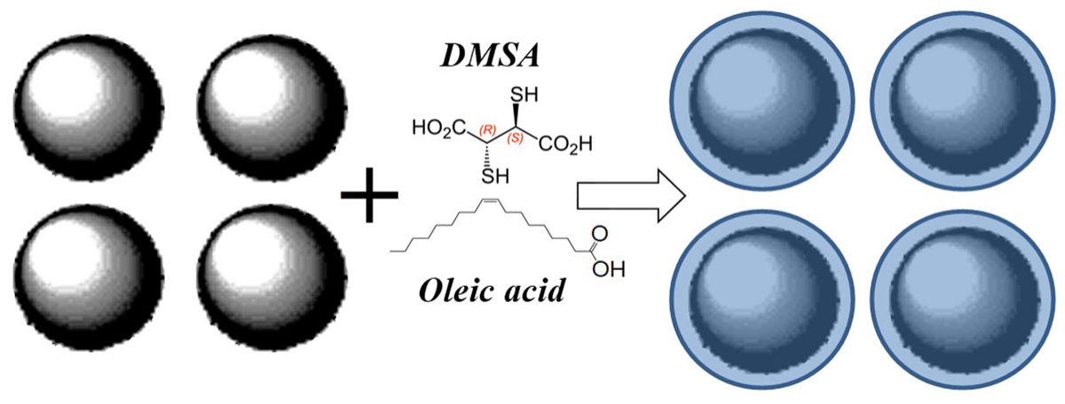
- Oshtrakh, M.I.; Ushakov, M.V.; Semionkin, V.A.; Lima, E.C.D.; Morais, P.C. Study of maghemite nanoparticles as-prepared and coated with DMSA using Mössbauer spectroscopy with a high velocity resolution. Hyperfine Interact. 2014, 226, 123–130. [Google Scholar] [CrossRef]
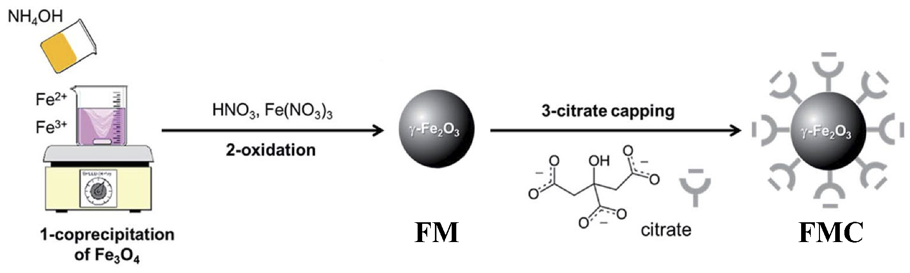
- Ushakov, M.V.; Sousa, M.H.; Morais, P.C.; Kuzmann, E.; Semionkin, V.A.; Oshtrakh, M.I. Effect of iron oxide nanoparticles functionalization by citrate analyzed using Mössbauer spectroscopy. Hyperfine Interact. 2020, 241, 27. [Google Scholar] [CrossRef]
- Oshtrakh, M.I.; Ushakov, M.V.; Senthilkumar, B.; Kalai Selvan, R.; Sanjeeviraja, C.; Semionkin, V.A. Iron environment non-equivalence in both octahedral and tetrahedral sites in NiFe2O4 nanoparticles: Study using Mössbauer spectroscopy with a high velocity resolution. In Proceedings of the International Conference “Mössbauer Spectroscopy in Materials Science 2012”, Olomouc, Czech Republic, 11–15 June 2012; Tuček, J., Machala, L., Eds.; AIP Publishing: Melville, NY, USA, 2012; Volume 1489, pp. 115–122. [Google Scholar]
- Oshtrakh, M.I.; Ushakov, M.V.; Senthilkumar, B.; Kalai Selvan, R.; Sanjeeviraja, C.; Felner, I.; Semionkin, V.A. Study of NiFe2O4 nanoparticles using Mössbauer spectroscopy with a high velocity resolution. Hyperfine Interact. 2013, 219, 7–12. [Google Scholar] [CrossRef] [Green Version]
- Ushakov, M.V.; Senthilkumar, B.; Kalai Selvan, R.; Felner, I.; Oshtrakh, M.I. Mössbauer spectroscopy of NiFe2O4 nanoparticles: The effect of Ni2+ in the Fe3+ local microenvironment in both tetrahedral and octahedral sites. Mater. Chem. Phys. 2017, 202, 159–168. [Google Scholar] [CrossRef]
- Ramalho, M.A.F.; Gama, L.; Antonio, S.G.; Paiva-Santos, C.O.; Miola, E.J.; Kiminami, R.H.G.A.; Costa, A.C.F.M. X-ray diffraction and Mössbauer spectra of nickel ferrite prepared by combustion reaction. J. Mater. Sci. 2007, 42, 3603–3606. [Google Scholar] [CrossRef]
- Yu, B.Y.; Kwak, S.-Y. Self-assembled mesoporous Co and Ni-ferrite spherical clusters consisting of spinel nanocrystals prepared using a template-free approach. Dalton Trans. 2011, 40, 9989–9998. [Google Scholar] [CrossRef]
- Mahmoud, M.H.; Elshahawy, A.M.; Makhlouf, S.A.; Hamdeh, H.H. Mössbauer and magnetization studies of nickel ferrite nanoparticles synthesized by the microwave-combustion method. J. Magn. Magn. Mater. 2013, 343, 21–26. [Google Scholar] [CrossRef]
- Ushakov, M.V.; Oshtrakh, M.I.; Chukin, A.V.; Šepelák, V.; Felner, I.; Semionkin, V.A. The milling effect on nickel ferrite particles studied using magnetization measurements and Mössbauer spectroscopy. Hyperfine Interact. 2018, 239, 4. [Google Scholar] [CrossRef]
- Kalai Selvan, R.; Augustin, C.O.; Oshtrakh, M.I.; Milder, O.B.; Semionkin, V.A. Mössbauer and d.c. magnetization studies of (CuFe2O4)1–x(SnO2)x (x = 0 and 5 wt.%) nanocomposites. Hyperfine Interact. 2005, 165, 231–237. [Google Scholar] [CrossRef]
- Kalai Selvan, R.; Augustin, C.O.; Oshtrakh, M.I.; Milder, O.B.; Semionkin, V.A. Hyperfine interactions in (CuFe2O4)1–x(SnO2)x (x = 0, 1, 5, 10 and 20 wt.%) nanocomposites studied by Mössbauer spectroscopy. Hyperfine Interact. 2007, 179, 33–38. [Google Scholar] [CrossRef]
- Jiang, J.Z.; Goya, G.F.; Rechenberg, H.R. Magnetic properties of nanostructured CuFe2O4. J. Phys. Condens. Matter. 1999, 11, 4063–4078. [Google Scholar] [CrossRef] [Green Version]
- Gajbhiya, N.S.; Balaji, G.; Bhattacharya, S.; Ghafari, M. Mössbauer studies of nanosize CuFe2O4 particles. Hyperfine Interact. 2004, 156–157, 57–61. [Google Scholar] [CrossRef]
- Al-Rawas, A.D.; Widatallah, H.M.; Al-Omari, I.A.; Johnson, C.; Elzain, M.E.; Gismelseed, A.M.; Al-Taie, S.; Yousif, A.A. The influence of mechanical milling and subsequent calcination on the formation of nanocrystalline CuFe2O4. In Proceedings of the International Symposium on the Industrial Applications of the Mössbauer Effect 2004, Madrid, Spain, 4–8 October 2004; Gracia, M., Marco, J.F., Plazaola, F., Eds.; AIP Publishing: Melville, NY, USA, 2005; Volume 765, pp. 277–281. [Google Scholar]
- Iqbal, M.J.; Yaqub, N.; Sepiol, B.; Ismail, B. A study of the influence of crystallite size on the electrical and magnetic properties of CuFe2O4. Mater. Res. Bull. 2011, 46, 1837–1842. [Google Scholar] [CrossRef]
- Kurian, J.; Mathew, M.J. Structural, optical and magnetic studies of CuFe2O4, MgFe2O4 and ZnFe2O4 nanoparticles prepared by hydrothermal/solvothermal method. J. Mag. Mag. Mater. 2018, 451, 121–130. [Google Scholar] [CrossRef]
- Oshtrakh, M.I.; Kalai Selvan, R.; Augustin, C.O.; Semionkin, V.A. Study of CuFe2O4–SnO2 nanocomposites by Mössbauer spectroscopy with high velocity resolution. Hyperfine Interact. 2008, 183, 34–37. [Google Scholar] [CrossRef]
- Kalai Selvan, R.; Augustin, C.O.; Berchmans, L.J.; Saraswathi, R. Combustion synthesis of CuFe2O4. Mater. Res. Bull. 2003, 38, 41–54. [Google Scholar] [CrossRef]
- Bloesser, A.; Kurz, H.; Timm, J.; Wittkamp, F.; Simon, C.; Hayama, S.; Weber, B.; Apfel, U.P.; Marschall, R. Tailoring the size, inversion parameter, and absorption of phase-pure magnetic MgFe2O4 nanoparticles for photocatalytic degradations. ACS Appl. Nano Mater. 2020, 3, 11587–11599. [Google Scholar] [CrossRef]
- Ushakov, M.V.; Nithya, V.D.; Rajeesh Kumar, N.; Arunkumar, S.; Chukin, A.V.; Kalai Selvan, R.; Oshtrakh, M.I. X-ray diffraction, magnetic measurements and Mössbauer spectroscopy of MgFe2O4 nanoparticles. J. Alloys Comp. 2022, 912, 165125. [Google Scholar] [CrossRef]
- Ounnunkad, S.; Winotai, P.; Phanichphant, S. Cation distribution and magnetic behavior of Mg1−xZnxFe2O4 ceramics monitored by Mössbauer spectroscopy. J. Electroceram. 2006, 16, 363–368. [Google Scholar] [CrossRef]
- Sivakumar, N.; Narayanasamy, A.; Grenèche, J.-M.; Murugaraj, R.; Lee, Y.S. Electrical and magnetic behaviour of nanostructured MgFe2O4 spinel ferrite. J. Alloys Comp. 2010, 504, 395–402. [Google Scholar] [CrossRef]
- Gismelseed, A.M.; Mohammed, K.A.; Elzain, M.E.; Widatallah, H.M.; Al-Rawas, A.D.; Yousif, A.A. The structural and magnetic behaviour of the MgFe2−xCrxO4 spinel ferrite. Hyperfine Interact. 2012, 208, 33–37. [Google Scholar] [CrossRef]
- Yoshizawa, Y.; Oguma, S.; Yamauchi, K. New Fe-based soft magnetic alloys composed of ultrafine grain structure. J. Appl. Phys. 1988, 64, 6044–6046. [Google Scholar] [CrossRef]
- Kuzmann, E.; Stichleutner, S.; Sápi, A.; Varga, L.K.; Havancsák, K.; Skuratov, V.; Homonnay, Z.; Vértes, A. Mössbauer study of FINEMET type nanocrystalline ribbons irradiated with swift heavy ions. Hyperfine Interact. 2012, 207, 73–79. [Google Scholar] [CrossRef]
- Kuzmann, E.; Stichleutner, S.; Machala, L.; Pechousek, J.; Vondrasek, R.; Smrcka, D.; Kouril, L.; Homonnay, Z.; Oshtrakh, M.I.; Mozzolai, A.; et al. Change in magnetic anisotropy at the surface and in the bulk of FINEMET induced by swift heavy ion irradiation. Nanomaterials 2022, 12, 1962. [Google Scholar] [CrossRef]
- Kuzmann, E.; Stichleutner, S.; Sápi, A.; Klencsár, Z.; Oshtrakh, M.I.; Semionkin, V.A.; Kubuki, S.; Homonnay, Z.; Varga, L.K. Mössbauer study of FINEMET with different permeability. Hyperfine Interact. 2013, 219, 63–67. [Google Scholar] [CrossRef] [Green Version]
- Oshtrakh, M.I.; Klencsar, Z.; Semionkin, V.A.; Kuzmann, E.; Homonnay, Z.; Varga, L.K. Annealed FINEMET ribbons: Structure and magnetic anisotropy as revealed by the high velocity resolution Mössbauer spectroscopy. Mat. Chem. Phys. 2016, 180, 66–74. [Google Scholar] [CrossRef]
- Borrego, J.M.; Conde, A.; Pena-Rodríguez, V.A.; Grenèche, J.M. Mössbauer spectrometry of FINEMET-type nanocrystallibe alloy. Hyperfine Interact. 2000, 131, 67–82. [Google Scholar] [CrossRef]
- Crisan, O.; Le Breton, J.M.; Filoti, G. Nanocrystallization of soft magnetic Finemet-type amorphous ribbons. Sens. Actuat. A 2003, 106, 246–250. [Google Scholar] [CrossRef]


| Sample | T, K | Γ, mm/s | δ, mm/s | ΔEQ (2ε), mm/s | Heff, kOe | A, % | Spectral Component |
|---|---|---|---|---|---|---|---|
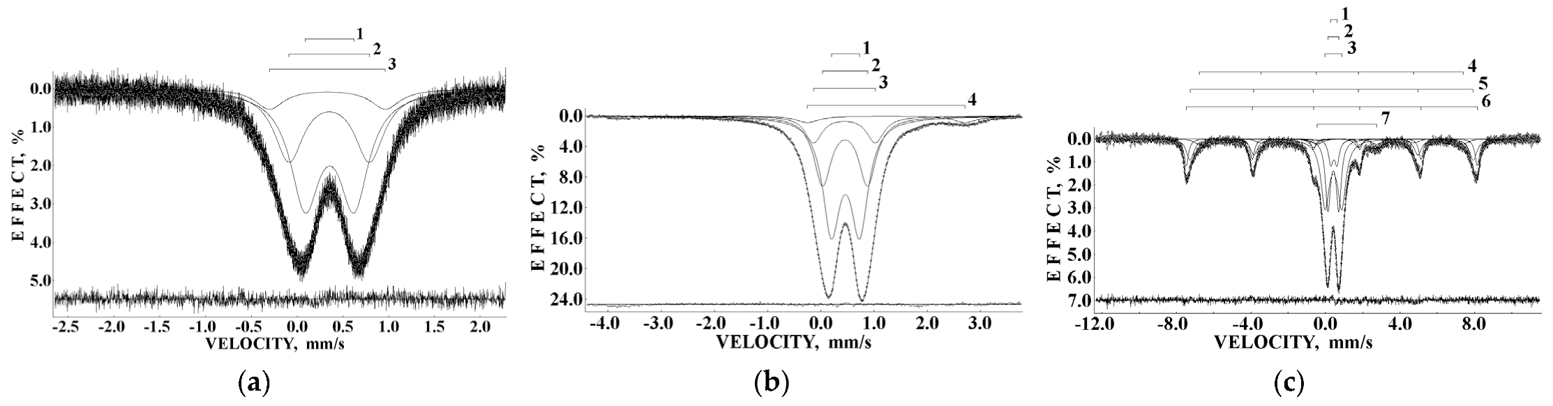
| Imferon | 295 | 0.390 ± 0.009 | 0.356 ± 0.003 | 0.534 ± 0.015 | – | 55.22 | 1 (FeOOH) |
| (lyophilized) | 0.390 ± 0.009 | 0.352 ± 0.003 | 0.880 ± 0.030 | – | 34.89 | 2 (FeOOH) | |
| 0.390 ± 0.009 | 0.331 ± 0.009 | 1.268 ± 0.043 | – | 9.90 | 3 (FeOOH) | ||
| Imferon | 87 | 0.396 ± 0.032 | 0.465 ± 0.016 | 0.530 ± 0.016 | – | 51.84 | 1 (FeOOH) |
| (frozen solution) | 0.396 ± 0.032 | 0.457 ± 0.016 | 0.844 ± 0.016 | – | 31.59 | 2 (FeOOH) | |
| 0.396 ± 0.032 | 0.444 ± 0.016 | 1.160 ± 0.016 | – | 12.43 | 3 (FeOOH) | ||
| 0.543 ± 0.032 | 1.228 ± 0.016 | 2.966 ± 0.018 | – | 4.13 | 4 (FeCl2) | ||
| Imferon | 90 | 0.298 ± 0.024 | 0.452 ± 0.012 | 0.330 ± 0.012 | – | 6.14 | 1 (FeOOH) |
| (frozen solution) | 0.323 ± 0.024 | 0.424 ± 0.012 | 0.580 ± 0.012 | – | 19.01 | 2 (FeOOH) | |
| 0.537 ± 0.024 | 0.427 ± 0.012 | 0.889 ± 0.012 | – | 30.53 | 3 (FeOOH) | ||
| 0.694 ± 0.073 | 0.473 ± 0.017 | −0.329 ± 0.035 | 440.0 ± 2.2 | 7.06 | 4 (FeOOH) | ||
| 0.489 ± 0.028 | 0.449 ± 0.012 | −0.220 ± 0.012 | 472.0 ± 0.6 | 19.26 | 5 (FeOOH) | ||
| 0.292 ± 0.024 | 0.471 ± 0.012 | −0.257 ± 0.012 | 485.2 ± 0.5 | 14.56 | 6 (FeOOH) | ||
| 0.705 ± 0.080 | 1.148 ± 0.027 | 3.199 ± 0.051 | – | 3.44 | 7 (FeCl2) |
Publisher’s Note: MDPI stays neutral with regard to jurisdictional claims in published maps and institutional affiliations. |
© 2022 by the authors. Licensee MDPI, Basel, Switzerland. This article is an open access article distributed under the terms and conditions of the Creative Commons Attribution (CC BY) license (https://creativecommons.org/licenses/by/4.0/).
Share and Cite
Alenkina, I.V.; Ushakov, M.V.; Morais, P.C.; Kalai Selvan, R.; Kuzmann, E.; Klencsár, Z.; Felner, I.; Homonnay, Z.; Oshtrakh, M.I. Mössbauer Spectroscopy with a High Velocity Resolution in the Studies of Nanomaterials. Nanomaterials 2022, 12, 3748. https://doi.org/10.3390/nano12213748
Alenkina IV, Ushakov MV, Morais PC, Kalai Selvan R, Kuzmann E, Klencsár Z, Felner I, Homonnay Z, Oshtrakh MI. Mössbauer Spectroscopy with a High Velocity Resolution in the Studies of Nanomaterials. Nanomaterials. 2022; 12(21):3748. https://doi.org/10.3390/nano12213748
Chicago/Turabian StyleAlenkina, Irina V., Michael V. Ushakov, Paulo C. Morais, Ramakrishan Kalai Selvan, Ernő Kuzmann, Zoltán Klencsár, Israel Felner, Zoltán Homonnay, and Michael I. Oshtrakh. 2022. "Mössbauer Spectroscopy with a High Velocity Resolution in the Studies of Nanomaterials" Nanomaterials 12, no. 21: 3748. https://doi.org/10.3390/nano12213748