Article

Particle Distribution and Heat Transfer of SiO2/Water Nanofluid in the Turbulent Tube Flow

1
State Key Laboratory of Fluid Power Transmission and Control, Zhejiang University, Hangzhou 310027, China
2
Faculty of Mechanical Engineering and Mechanics, Ningbo University, Ningbo 315201, China
*
Author to whom correspondence should be addressed.
Nanomaterials 2022, 12(16), 2803; https://doi.org/10.3390/nano12162803
Submission received: 12 July 2022 / Revised: 28 July 2022 / Accepted: 10 August 2022 / Published: 15 August 2022
(This article belongs to the Special Issue Applications of Nanofluids – II)

Abstract

:
In order to clarify the effect of particle coagulation on the heat transfer properties, the governing equations of nanofluid together with the equation for nanoparticles in the SiO2/water nanofluid flowing through a turbulent tube are solved numerically in the range of Reynolds number 3000 ≤ Re ≤ 16,000 and particle volume fraction 0.005 ≤ φ ≤ 0.04. Some results are validated by comparing with the experimental results. The effect of particle convection, diffusion, and coagulation on the pressure drop ∆P, particle distribution, and heat transfer of nanofluid are analyzed. The main innovation is that it gives the effect of particle coagulation on the pressure drop, particle distribution, and heat transfer. The results showed that ∆P increases with the increase in Re and φ. When inlet velocity is small, the increase in ∆P caused by adding particles is relatively large, and ∆P increases most obviously compared with the case of pure water when the inlet velocity is 0.589 m/s and φ is 0.004. Particle number concentration M0 decreases along the flow direction, and M0 near the wall is decreased to the original 2% and decreased by about 90% in the central area. M0 increases with increasing Re but with decreasing φ, and basically presents a uniform distribution in the core area of the tube. The geometric mean diameter of particle GMD increases with increasing φ, but with decreasing Re. GMD is the minimum in the inlet area, and gradually increases along the flow direction. The geometric standard deviation of particle diameter GSD increases sharply at the inlet and decreases in the inlet area, remains almost unchanged in the whole tube, and finally decreases rapidly again at the outlet. The effects of Re and φ on the variation in GSD along the flow direction are insignificant. The values of convective heat transfer coefficient h and Nusselt number Nu are larger for nanofluids than that for pure water. h and Nu increase with the increase in Re and φ. Interestingly, the variation in φ from 0.005 to 0.04 has little effect on h and Nu.

1. Introduction

Convective heat transfer plays an important role in industrial and heating/cooling equipment [1]. Enhancing heat transfer to improve the efficiency of heat exchangers is an important research direction. The flow characteristics [2] and geometry of heat transfer surfaces [3,4] are important factors affecting convective heat transfer. Nanoparticles have many important uses [5], for example, it is more effective to add nanoparticles into the fluid (i.e., nanofluid) to improve its thermal conductivity and convective heat transfer coefficient, so as to achieve the purpose of enhancing heat transfer.
The studies on convective heat transfer in nanofluids have been reported in previous research. Ramesh et al. [6] studied the flow and heat transport structures of Al2O3-Ag and Al2O3-Cu hybrid nanoparticles in a moving material and observed that the skin friction value of the Al2O3-Cu/water case was lower in comparison to the values of the Nusselt number for Al2O3-Ag/water nanoparticles. Ali et al. [7] studied the convective heat transfer of nanofluids with different SiO2 volume concentrations in a horizontal tube and found a significant increase in heat transfer with increasing particle concentration. Hejazian et al. [8] used the Euler model and mixture model to study the forced convection of a nanofluid in a tube with a wall exposed to the saturated steam; the results showed that the estimation of convective heat transfer by the hybrid model was in better agreement with the experimental results in the range of Reynolds number 3000 ≤ Re ≤ 14,000 and volume concentration 0.1% ≤ Vc ≤ 2%.
The effect of the shape and size of the particles on the heat transfer has also been investigated. Liu et al. [9] introduced two new shape parameters, flatness and elongation, to study the effect of non-spherical particles on the heat transfer and established a new modified model for the correlation of Nusselt numbers related to particle shape, size, and volume fraction. Hemmat and Saedodin [10] conducted the empirical study on heat transfer and thermophysical properties considering different diameters of MgO nanoparticles, and the results showed that the traditional formulation underestimated the thermophysical parameters such as thermal conductivity and dynamic viscosity. They also found that the smaller the diameter of the nanoparticle, the higher the thermal conductivity and kinetic viscosity, and the larger the convective heat transfer coefficient. Keblinski et al. [11] gave four explanations for the increase in the thermal conductivity with decreasing nanoparticle scale, namely, the Brownian motion of the nanoparticles, the molecular layer of the liquid at the liquid and particle interfaces, the nature of heat transfer in the nanoparticles, and particle aggregation. Bahiraei also [12] demonstrated the effect of the thermophoretic force and the Brownian force on the convection heat exchange through numerical simulation and found that its effect was more obvious far from the pipe inlet. Heyhat and Kowsary [13] used the Buongiorno model to study the flow of Al2O3-water nanofluid through a pipeline, and found that compared with the uniform volume fraction, the heat transfer coefficient increased; thus, realizing the same enhanced convection heat transfer.
Lin et al. [14,15] analyzed the characteristic of heat transfer in the flow of nanofluids with spherical and rod-like nanoparticles and found that it was more effective to enhance the heat transfer for the rod-like nanoparticles with larger aspect ratio at the flow with higher Reynolds number. Zhang [16] studied the heat transfer in a turbulent curved tube and found that the energy performance evaluation standard ratio of Al2O3/water nanofluid to base fluid increased with the increase in Reynolds number, volume fraction, and Dean number, but with the decrease in Schmidt number. Calvino et al. [17] analyzed experimentally the convective heat transfer performance of a polycarboxylate chemically modified GnP dispersion in water at 0.50 wt% and obtained the convective heat transfer coefficients reaching enhancements for the nanofluid of up to 13%. Alam et al. [18] presented the experimental forced convective heat transfer coefficient of nanorods zinc oxide–ethylene glycol nanofluids in laminar flow. The results showed that adding only small amounts of zinc oxide nanorods to ethylene glycol could significantly increase the heat transfer coefficient.
At present, there are some models and solutions for nanofluids. Jamshed et al. [19] chose the Prandtl–Eyring hybrid nanofluid as a working fluid in the solar water pump model for the production of a solar water pump in a parabolic trough surface collector. Shahzad et al. [20] developed models for coronavirus disease at different stages with the addition of more parameters due to interactions among the individuals and computed the local sensitivities for each model state concerning the model parameters using the model reduction techniques. Abdullah et al. [21] developed a new mathematical model by including the resistive class together with the quarantine class and used it to investigate the transmission dynamics of the novel coronavirus disease.
By reviewing previous relevant research, it can be seen that the there are few studies on the nanoparticle coagulation in the nanofluids and resulting distribution of particles, and the research on the effect of particle coagulation on the heat transfer characteristics is lacking. However, nanoparticle coagulation is a common phenomenon in nanofluid flow. After nanoparticle coagulation, the number and size of particles in the flow will be changed, which will affect the pressure drop and heat transfer. Therefore, in the present work, we study numerically the momentum and energy equations of nanofluids together with the population balance equation for nanoparticles in the SiO2/water nanofluid flowing through a turbulent tube and explore the effect of particle coagulation on the pressure drop, particle distribution, and heat transfer of SiO2/water nanofluids.

2. Basic Equations

The turbulent tube flow of nanofluids with SiO2 nanoparticles is simulated numerically with saturated steam wall exposure (convective boundary conditions). We chose SiO2 as the nanoparticles because it is insoluble in water and has good dispersion and stability in water. Figure 1 shows the geometry of the tube with a diameter D = 0.0064 m and length L = 1.5 m. The tube is made of copper material and has a wall thickness of 0.0008 m.

2.1. Equations for the Nanofluid

The nanofluid is the mixture of the base liquid with the nanoparticles. The governing equations for the nanofluid are expressed as [22,23]:
ρ n f u i x i = 0
t ρ n f u i + x j ρ n f u i u j = p x i + x j μ n f u i x j + u j x i + x j ρ n f u i u j ¯
t ( ρ n f E ) + x i u i ( ρ n f E + p ) = x j k n f + c p , n f μ t Pr t T x j
where E is total energy E = c p , n f T ( P / ρ n f ) + u 2 / 2 ; T is nanofluid temperature; ρ n f , μ n f , c p , n f , k n f are density, dynamic viscosity, specific heat capacity, and thermal conductivity of the nanofluid, respectively; ui is nanofluid velocity. The last term on the right-hand side of Equation (2) is the Reynolds stress Rij [15]:
R i j = ρ n f u i u j ¯ = μ t u i x j + u j x i 2 3 ρ n f k δ i j 2 3 μ t u k x k δ i j
where μt is turbulent dynamical viscosity and δ is the Kronecker function.
The equations for the turbulent dissipation rate ω and turbulent kinetic energy k are given by [3,24]:
d d t ( ρ ω ) = ρ D ω ω + ρ γ G ν t 2 3 ρ γ ω ( u ) ρ β ω 2 ρ F 1 1 C D k ω + S ω
d d t ( ρ k ) = ρ D k k + ρ G 2 3 ρ k ( u ) ρ β * ω k + S k
where G is turbulent kinetic energy generation rate due to the anisotropic part of the Reynolds stress tensor; Dk, Dω represent the effective diffusion of k and ω; Sk, Sω are the internal source terms of k and ω; the turbulent kinematic viscosity is obtained by:
ν t = a 1 k max a 1 ω , b 1 F 2 S
where S is a measure of the strain rate tensor, the other default model constants are listed in Table 1, and the auxiliary relationships are as follows:
F 1 = tanh min max k β * ω y , 500 v y 2 ω , 4 ρ σ ω 2 k C D k ω y 2 4 , C D k w = max 2 ρ σ ω 2 1 ω k x i ω x i , 10 10 F 2 = tanh max 2 k β * ω y , 500 v y 2 ω 2 , G = ρ u i u j ¯ u j / x i , γ = γ 1 F 1 + γ 2 1 F 1 D k = μ + μ t α k , D ω = μ + μ t α ω α k = 1 F 1 / α k 1 + 1 F 1 / α k 2 , α ω = 1 F 1 / α ω 1 + 1 F 1 / α ω 2

2.2. Population Balance Equation for Nanoparticles

The population balance equation essentially explains the various ways in which state-specific particles form or disappear from the system [25]. The population balance equation obtained by considering the evolution of nanoparticles under convection, diffusion, and coagulation is:
n v , t t + u n v , t D B + ν t n v , t = 1 2 0 v β ( v 1 , v v 1 ) n v 1 , t n v v 1 , t d v 1 0 β ( v 1 , v ) n v 1 , t n v , t d v 1
where n ( v , t ) is particle size distribution function, reflecting the spatial distribution of the number of particles with a volume of v at time t; the diffusion coefficient caused by the particle Brownian motion is expressed as D B = k B T / 3 π μ n f d p ; β ( v 1 , v ) is coagulation kernel function of two particles with volumes of v and v 1 under the action of collision, and the coagulation of nanoparticles mainly results from particle Brownian motion.
The particle distribution in the above equations should be solved for the systems with different particle types, so the computational cost is too high. For this reason, the moment method, the partition method, and the Monte Carlo method are developed, among which the moment method is most commonly used, but it needs to solve the problem of equation closure. The integral moment method for the equilibrium equation of particles is collated by Li et al. [26]. According to the concept of the moment method proposed by Hulbert and Katz [27], the moment is defined as m k = 0 n v , t v k d v , and the k-order moment equation of the particle size distribution obtained by integrating Equation (8) is:
m k t + u i m k x i x i D B + ν t m k x i = 1 2 0 0 v + v 1 k v k v 1 k β ( v 1 , v ) n ( v , t ) n ( v 1 , t ) d v d v 1
The distribution of particles in the gas medium can be divided into free molecular zones, transition zones, sliding zones, and continuous zones according to different Knudsen numbers (the ratio of the mean free path to the particle diameter) [28]. However, the mean free path of liquid molecules in solid–liquid systems is the same as the radius of 0.1 nm particle scale, and nanoparticles in a liquid can usually be modeled with standard continuum theory. The expression of the corresponding particle coagulation kernel function is:
β ( v 1 , v ) = 2 k B T 3 μ n f 1 v 1 / 3 + 1 v 1 1 / 3 v 1 / 3 + v 1 1 / 3
By substituting Equation (10) into Equation (9) and closing the moment equation with Taylor’s series approximation technique [29] which is an effective method [30,31], we obtain the first three closed moment equations as follows:
m 0 t + u i m 0 x i x i D B + ν t m 0 x i = 2 k B T 3 μ n f 2 m 0 4 m 2 2 13 m 0 3 m 1 2 m 2 151 m 0 2 m 1 4 81 m 1 4
m 1 t + u i m 1 x i x i D B + ν t m 1 x i = 0
m 2 t + u i m 2 x i x i D B + ν t m 2 x i = 4 k B T 3 μ n f 2 m 0 4 m 2 2 13 m 0 m 1 2 m 2 151 m 1 4 81 m 1 2

2.3. Thermophysical Parameters of the Nanofluid

In this study, the properties of the basic fluid and the nanoparticles are assumed to be unchanged with temperature, and the thermophysical parameters of the material are shown in Table 2.
The effective density and specific heat capacity of nanofluid are given by the concept of hybrid theory commonly used [32,33]:
ρ n f = φ ρ p + ( 1 φ ) ρ f
c p , n f = φ c p , p ρ p + ( 1 φ ) ρ f c p , f ρ n f  
where ρ f , ρ p are densities of the base fluid and nanoparticles at temperature 298 K, respectively; c p , f , c p , p are the specific heat capacities of the base fluid and nanoparticles, respectively; φ is the volume fraction of the nanoparticles.
The properties of heat transfer in the nanofluid are improved by reducing the heat resistance when adding nanoparticles of high thermal conductivity to the basic fluid. The calculation of the thermal conductivity and dynamic viscosity has developed different expressions in terms of theoretical and empirical corrections [34,35,36]. The effective thermal conductivity of the classical Maxwell theory model is calculated by:
k n f = k p + 2 k f + 2 φ k p k f k p + 2 k f φ k p k f k f
where k f , k p are thermal conductivity of the base fluid and nanoparticles, respectively.
Experimental results of nanofluid viscosity incorporating particles of different sizes, shapes, and volume fractions showed that the Einstein equation is significantly underestimated by the increased viscosity as commonly used in the literature [37]. Therefore, the experimental modified model proposed by Corcione [38] with relatively small error is used to predict effective viscosity:
μ n f = μ f 1 34.87 ( d p / d f ) 0.3 φ 1.03
where μf is dynamic viscosity of the base fluid; dp is nanoparticle diameter; df is equivalent diameter of the base fluid molecule given by d f = 6 M / N A π ρ f 1 / 3 , where M is molecular weight of the base fluid (18 g/mol) and NA is Avogadro constant (6.022140857 × 10²³ mol−1).
Reynolds number and Prandtl number of nanofluids are Re = ρ n f u i n D / μ n f and Pr = μ n f C p , n f / k n f . Table 3 summarizes the parameters of nanofluids at different volume fractions.

3. Numerical Method and Verification

3.1. Numerical Method

To solve the above-mentioned system of control equations, a solver is customized on the OpenFoam platform based on the finite volume method. The SIMPLE algorithm is used to solve the coupling problem of velocity and pressure, and to synchronize the velocity field and temperature field solved in the flow to the moment Equation (11–13) to obtain the information of the particle field. The time term in the equation is discretized in the Euler scheme, the gradient term is a Gaussian linear dispersion, the vector convection term is treated in the Gauss linear upwind limited scheme, and the scalar transport convection term is treated in the Gauss limited linear way.
In the computation, the O-type hexahedron structured mesh division method is adopted for the tube. The grid nodes on the square edge of the section core are evenly distributed, the square vertex to the circular wall grid node b is unevenly distributed, the grid near the wall is tighter, and the axis-up grid node c is evenly distributed.

3.2. Boundary Condition

The boundary conditions used to solve the equations are as follows:
  • Inlet
The boundary condition for velocity is selected, the inlet temperature is set to be 298K, and the volume fraction of the particles is uniform.
2.
Wall
No-slip boundary condition is used for velocity. For the outside of the wall and the sub-saturated steam contact, the ambient temperature Tsteam = 351 K, and the heat transfer coefficient for steam hsteam = 12,000 W/m2K. The volume fraction of the particles is zero gradient
3.
Outlet
The gradient of each parameter at the outlet is zero.

3.3. Parameter Definition

The pressure drop ∆P from inlet to outlet is defined as:
Δ P = P in P out
The convective heat transfer coefficient h and Nusselt number Nu are defined as:
h = ρ C p nf A u T out T in π D L T w T b ,   Nu = h D k nf
where A is cross-sectional area of the tube; T w , T i n , T o u t , T b are mean wall temperature, mean inlet temperature, mean outlet temperature, and volume temperature, respectively, T b = T in + T out / 2 .

3.4. Main Steps of the Numerical Simulation

(1)
Solve Equations (1)–(7) with φ = 0 to get ui.
(2)
Solve Equations (11)–(13) to get m0, m1, and φ .
(3)
Substitute φ into Equations (14)–(17) to get ρnf, cp,nf, knf, and μnf.
(4)
Substitute φ , ρnf, cp,nf, knf, and μnf into Equations (1)–(7), and solve the equations to get ui, p, and T.
(5)
Repeat steps (2) to (4) based on the new flow velocity ui until the difference between the successive results of ui, p, and T is less than a definite value.
(6)
Calculate the pressure drop ∆P based on Equation (18), h and Nu based on Equation (19).

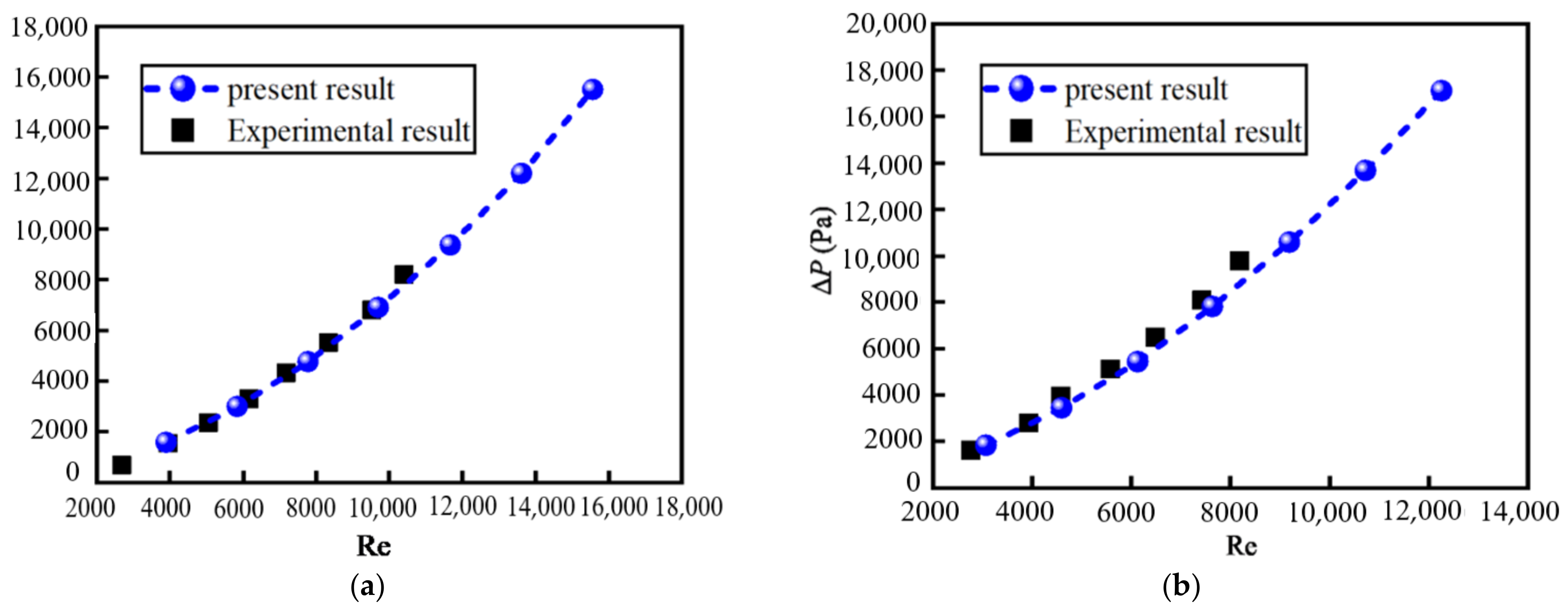
3.5. Grid Independence and Verification of Calculation Methods

The grid information and grid independence are shown in Table 4 where the pressure drop ∆P and convective heat transfer coefficient h are shown. The comparison of ∆P and hmean shows that the deviation of ∆P and hmean is small for 20 × 15 × 1500 (Grid 2) and 24 × 18 × 1500 (Grid 3), the deviations of hmean and ∆P are within 0.06% and 0.6%, respectively. For 20 × 15 × 1500 (Grid 2) and 20 × 15 × 150 (Grid 4), the deviations of hmean and ∆P are within 0.5% and 0.2%, respectively. In order to balance the calculation time and accuracy, Grid 4 is selected for the following computation.
The variations in ∆P and mean heat transfer coefficient hmean with Reynolds number for pure water in the tube flow are shown in Figure 2 and Figure 3 where the present numerical results, experimental results [37], and Blasius solution (as seen in Equation (20)) are given as a comparison. We can see that the three results agree well.
Δ P = f L ρ n f u i n 2 / 2 D = 0.158 L ρ n f 0.75 μ n f 0.25 D 1.25 u i n 1.75

4. Results and Discussion

The equations are solved numerically in the range of Reynolds number 3000 ≤ Re ≤ 16,000 and particle volume fraction 0.005 ≤ φ ≤ 0.04. The selection of the range of Re and φ is based on the most common operating conditions in practical applications.

4.1. Pressure Drop

During the process of nanofluid flowing through the tube, energy loss will occur due to the action of viscous force. The empirical formula of the frictional coefficient is used to measure the energy loss. Nikuradse’s experiments on the flow with different tube diameters and flux revealed the law of flow energy loss in the tube and gave the relationship between the energy loss coefficient and the relative roughness as well as Reynolds number. Five regions were divided according to the Nikuradse’s experimental result, the region calculated in this paper belongs to the turbulent smooth region in which the energy loss coefficient along the tube is independent of the relative roughness, only related to the Reynolds number, and given by the Blasius formula f = 0.3164 Re 0.25 .
Figure 4 shows the relationship between the pressure drop ∆P and Reynolds number Re with different volume fractions φ of nanoparticles. The present numerical results are in good agreement with the experimental results [37]. The pressure decreases along the flow direction due to the energy loss when nanofluid flows through the tube. This energy loss is caused by overcoming the internal friction and the collision and momentum exchange between the fluid particles in the turbulent flow. The values of ∆P increase with the increase in Re. The higher the Re is, the more intense the collision and momentum exchange between the fluid particles is, the greater the energy loss is, so the larger ∆P is.
It can be seen from Figure 5 that, at the same inlet velocity, the values of ∆P increase significantly after adding nanoparticles because particles added in the base fluid would increase the flow resistance. ∆P is directly proportional to φ, which is attributed to the following two aspects: 1) the viscosity of the nanofluid increases with the increase in φ, which hinders the motion of the nanofluid; 2) irregular motion and migration of particles are enhanced with increasing φ. For a specific φ, the larger the inlet velocity is, the larger the value of ∆P is. In Equation (20), ∆P is proportional to the 1.75 power of the velocity in the turbulent smooth region. On the other hand, the larger the inlet velocity, the more intense the friction of the fluid with the tube wall, so the more energy is lost. When the inlet velocity is small, the increase in ∆P caused by adding particles is relatively large. The value of ∆P increases most obviously compared with the case of pure water when the inlet velocity is 0.589 m/s and φ is 0.004.

4.2. Particle Distribution

In addition to the influence of φ on the viscosity and heat transfer of nanofluids, the influence of particle size and shape is also considered. This means that we need to consider whether nanoparticles coagulate and thus change the particle size. Prasher [39] combined the coagulate kinetics of colloidal solutions at nanometer scale with heat transfer physics and found that the particle coagulation can explain the various abnormal phenomena observed in the experiment well, for example, the thermal conductivity of nanofluids has a peak value, and the dependence of thermal conductivity on temperature, time, and pH value increases with the increase in relative particle size.
Here, we analyze the particle distribution at different φ considering particle coagulation. At the inlet, the nanoparticles are single-mode monodisperse (monomers of the same size, and the initial particle diameter is the same), and the the particle diameters meet the logarithmic normal distribution at the outlet after particle coagulation [40]. The geometric mean diameter of the particle (GMD) and the geometric standard deviation of the diameter (GSD) are expressed as:
GMD = M 1 2 / M 0 3 M 2 1 / 3
GSD = exp ln M 0 M 2 / M 1 2 / 3
where M 0 , M 1 , M 2 are dimensionless particle number concentration, volume concentration, and the second moment of particles, respectively:
M 0 = m 0 / m 00 ,   M 1 = m 1 / m 10 ,   M 2 = m 2 / m 20
where m0 and m00 are the particle number concentration and initial particle number concentration; m1 and m10 are the volume concentration and initial volume concentration; m2 and m20 are the second moment and initial second moment, respectively.

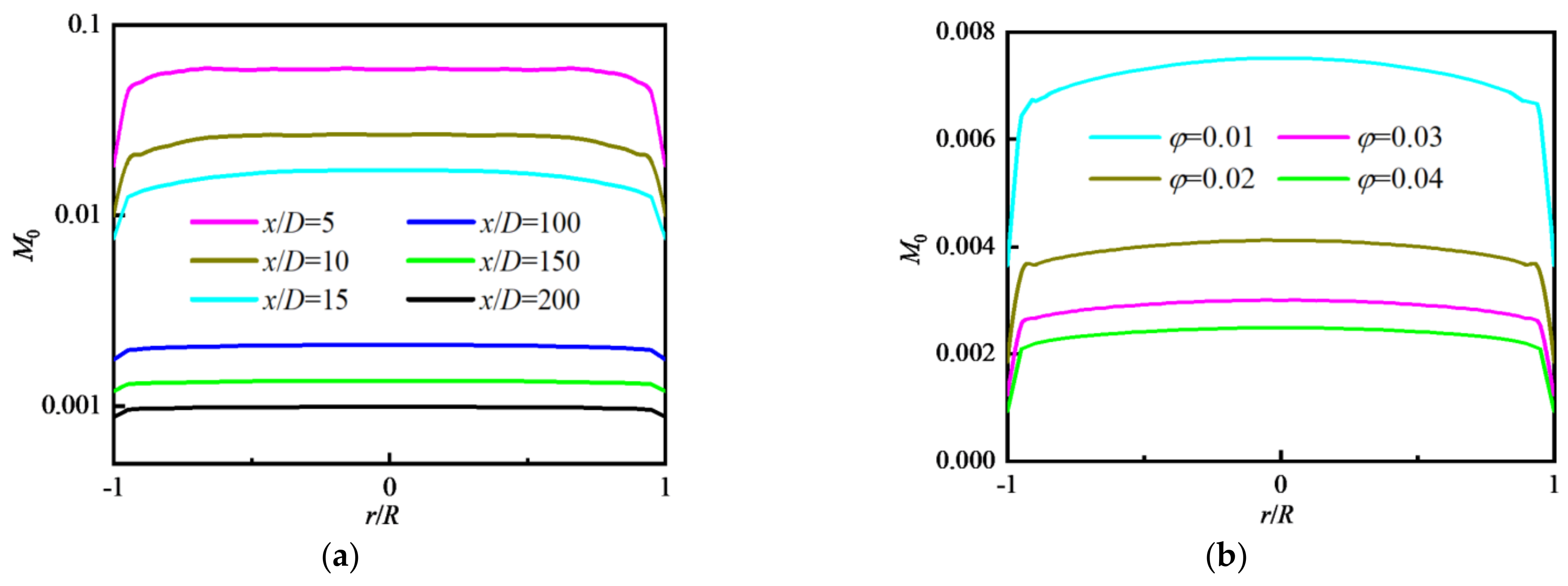
4.2.1. Distribution of Particle Number Concentration

The distribution of particle number concentration is determined using particle convection, diffusion, and coagulation. Particle convection and diffusion do not change the total particle number, but particle coagulation reduces the total particle number. The characteristic time of coagulation is very short. As shown in Equation (23), the zero-order moment M0 represents the particle number concentration. The distribution of M0 in the region of 0 ≤ x ≤ 5D is shown in Figure 6 where a significant reduction in M0 was observed because of particle coagulation. The value of M0 near the wall of the tube decreased to the original 2%, and it also decreased by about 90% in the central area of the tube.
Figure 7 shows the distribution of M0 along the flow direction under different Re and φ, respectively. M0 is averaged over the cross-section. It can be seen that M0 decreases along the flow direction, and the reduction rate gradually slows down. For a fixed φ, with the increase in Re, the values of M0 increase and the reduction rate of M0 along the flow direction decreases. Comparing the case with different φ, we can see that M0 increases with the increase in Re, while M0 decreases with the increase in φ because the larger the value of φ, the greater the probability of particle collision and coagulation, so the smaller the value of M0.
Figure 8 shows the distributions of M0 along the radial direction at different x/D and φ. In Figure 8a, the values of M0 are the largest in the inlet area of the tube (x/D = 5), and gradually decrease along the flow direction due to the particle coagulation. M0 in the core area basically presents a uniform distribution. In Figure 8b, the values of M0 decrease with the increase in φ, which is the same as the conclusion given in Figure 7.

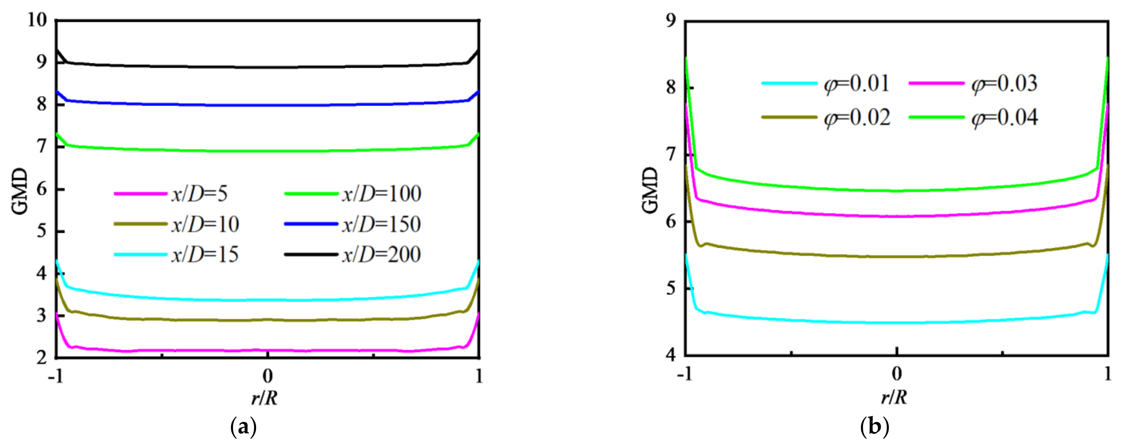
4.2.2. Distribution of Particle Diameter

The geometric mean diameter of particle (GMD) is defined in Equation (21). The particles with same size are initially distributed at the inlet, and the GMD will change because of coagulation when particles flow through the tube. The variation in GMD along the flow direction is shown in Figure 9a where φ = 0.01. We can see that GMD increases along the flow direction because of particle coagulation. GMD decreases with increasing Re, for example, the value of GMD for Re = 3793 is twice that of GMD for Re = 15,170 at the outlet. The reason is that the larger the Re is, the shorter the residence time of particles in the tube is, and the smaller the possibility of particle collision and coagulation is, so the smaller the value of GMD is. Figure 9b shows the variation in GMD along the flow direction when Re and φ change at the same time. It can be seen that the value of GMD increases with increasing φ, but with decreasing Re. In the case of large φ, the possibility of particle collision and coagulation is high, resulting in large GMD.
Figure 10 shows the distributions of GMD along the radial direction at different x/D and φ. In Figure 10a, the values of GMD are the minimum in the inlet area of the tube (x/D = 5), and gradually increase along the flow direction due to the particle coagulation. GMD in the core area basically presents a uniform distribution. In Figure 10b, the values of GMD increase with the increase in φ, which is the same as the conclusion given in Figure 9b.

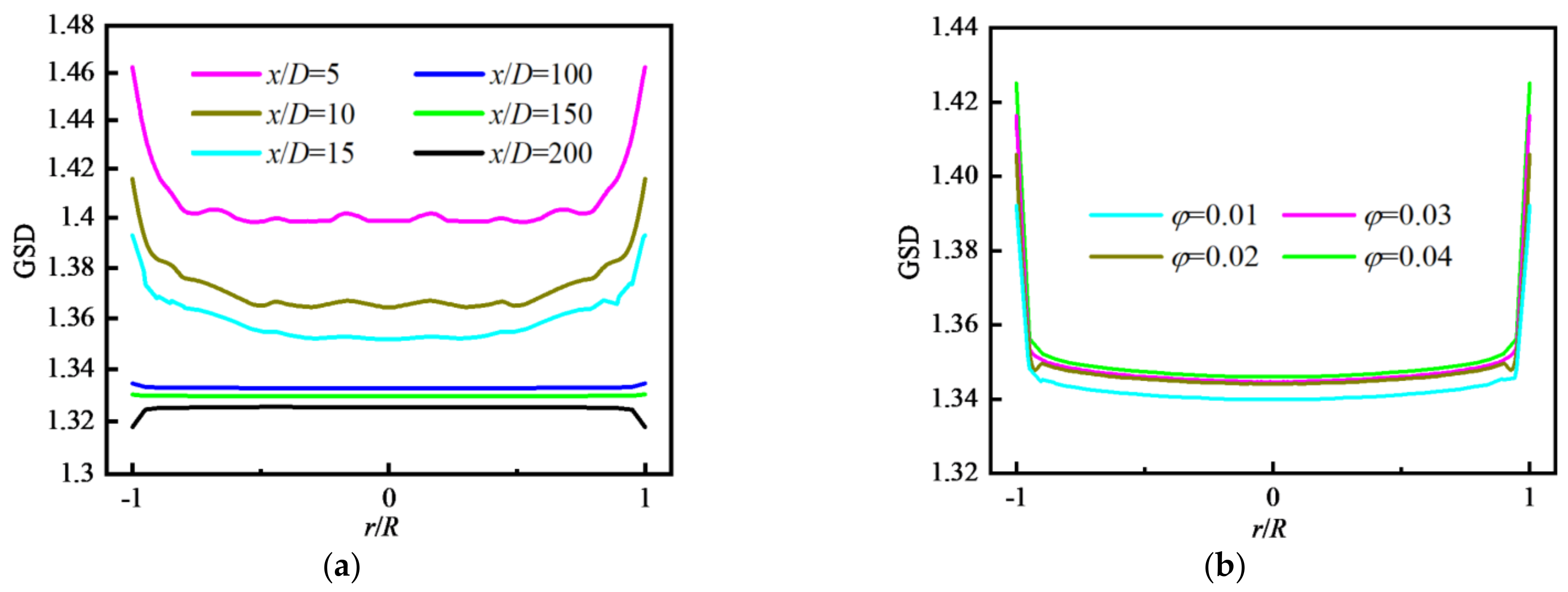
4.2.3. Distribution of Particle Polydispersity

For an initially monodisperse particle field at the inlet, the particle coagulation will result in the change in particle diameter and make the particle field become polydisperse along the tube. The geometric standard deviation of particle diameter (GSD) is defined in Equation (22). The variation in GSD along the flow direction is shown in Figure 11a where φ = 0.01. The values of GSD increase sharply at the inlet because the particle coagulation makes initially monodisperse particles change their sizes and particles become polydisperse when particles enter the tube, and then decrease in the inlet area of the tube (x/D < 5). Next, the values of GSD remain almost unchanged in the whole tube until at outlet where the values of GSD decrease rapidly again because of the influence of reflux. Figure 11b shows that the effects of Re and φ on the variation in GSD along the flow direction are insignificant.
Figure 12a shows the distributions of GSD along the radial direction at different x/D. In the inlet area of the tube (x/D < 15), the values of GSD decrease along the flow direction, and are unevenly distributed and fluctuate along the radial direction. Downstream (x/D > 100), the values of GSD change little along the flow direction and present a uniform distribution along the radial direction. The distributions of GSD along the radial direction for different φ are shown in Figure 12b where the φ has little effect on GSD except for the case of φ = 0.01.

4.3. Convective Heat Transfer

The convective heat transfer coefficient h and Nusselt number Nu are defined in Equation (19). Figure 13 and Figure 14 show the relationship between h, Nu, and Re for different φ. The values of h and Nu are larger for nanofluids than that for pure water (φ = 0), indicating that the addition of nanoparticles in pure water can improve the heat transfer performance, which is consistent with previous conclusions. The reasons for the enhancement of heat transfer performance are attributed to several aspects, for example, the thermal conductivity of the nanofluid is enhanced and hence carries more quantity of heat from the heated surface; mixing effects of particles near the wall; and disordered motion of nanoparticles.
We also can see that the values of h and Nu increase with the increase in φ, which is consistent with the result given by Ali et al. [7]. However, the change in h and Nu is not large from φ = 0.005 to φ = 0.04. The reason may be attributed to the fact that the possibility of particle collision and coagulation increases with increasing φ, resulting in the increase in particle size. Hemmat and Saedodin [10] indicated that the larger the diameter of the nanoparticle, the smaller the convective heat transfer coefficient. The increase in particle size partially counteracts the effect of heat transfer.
The values of h and Nu increase nearly linearly when Re changes from 3000 to 16,000. The relationship between h, Nu, and Re is consistent with previous conclusions [14,15,16]. The fact that the values of h and Nu are proportional to Re is attributed to the three factors: (1) the disordered movement of particles caused by the turbulent flow is more obvious at high Re, improving the heat transfer; (2) the laminar sublayer near the wall is thinner and the shear stress subsequently increases at high Re; and (3) a greater amount of heat is carried by a faster moving fluid at high Re than a slower moving fluid at low Re.

5. Conclusions

The momentum and energy equations of SiO2/water nanofluid, flowing through a turbulent tube, together with the population balance equation for nanoparticles were solved numerically with considering the particle convection, diffusion, and coagulation. Some results were validated by comparing with the experimental results. The effect of particle coagulation on the pressure drop ∆P, particle distribution, and heat transfer was explored. The main conclusions are summarized as follows:
(1)
P increases significantly after adding nanoparticles and increases with increasing Re. ∆P is proportional to particle volume fraction φ because increased viscosity hinders the motion of the nanofluid and more irregular migration of particles. For a specific φ, the larger the inlet velocity is, the larger the value of ∆P is. When inlet velocity is small, the increase in ∆P caused by adding particles is relatively large. The value of ∆P increases most obviously compared with the case of pure water when the inlet velocity is 0.589 m/s and φ is 0.004.
(2)
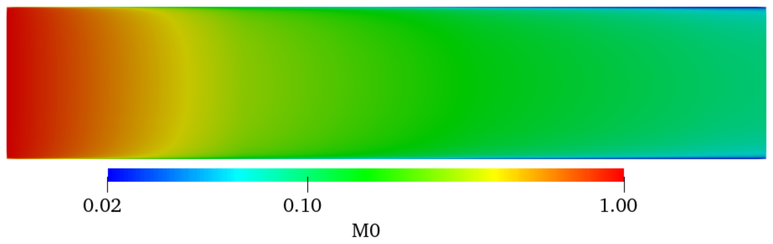
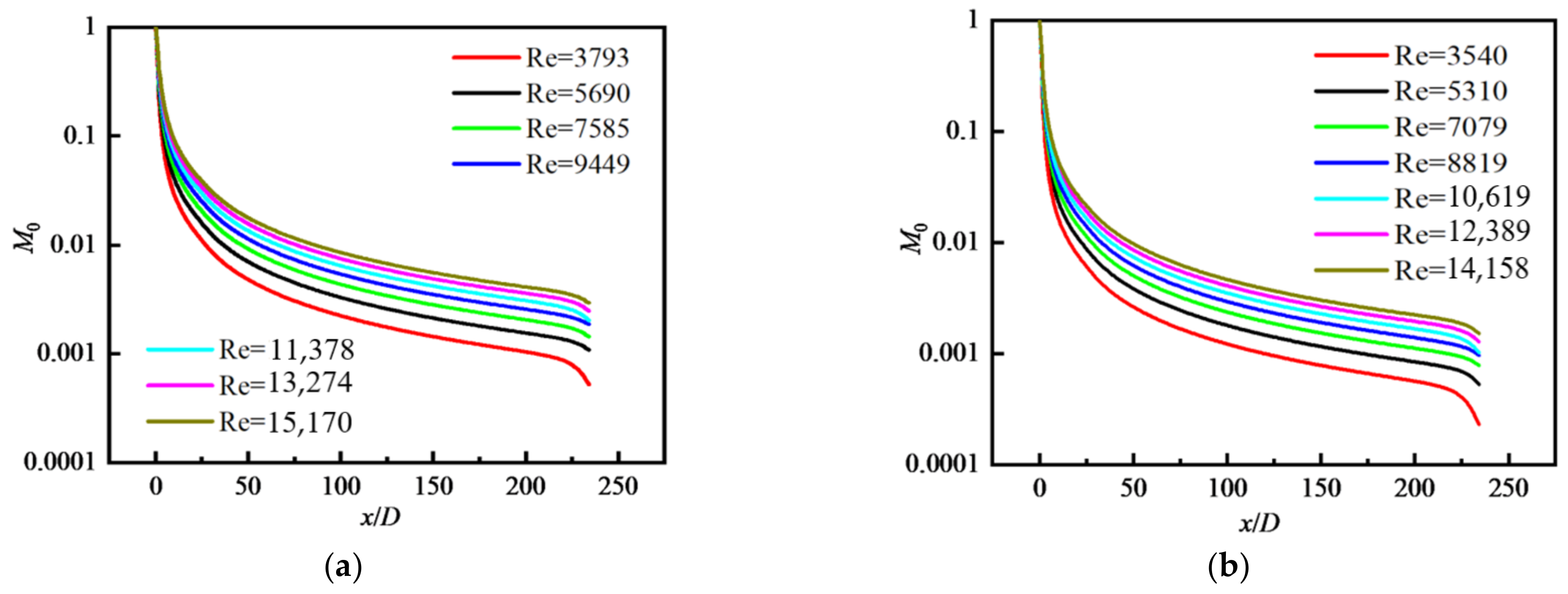
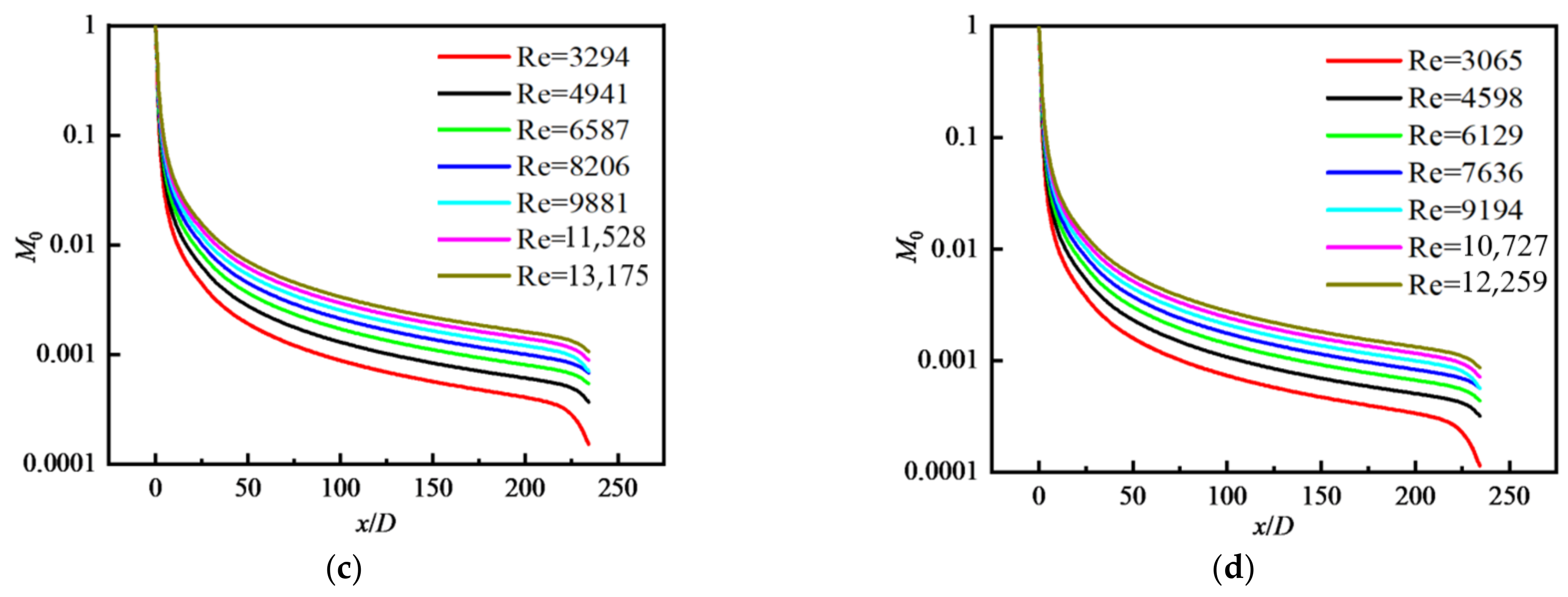
M0 decreases along the flow direction. M0 near the wall is decreased to the original 2% and decreased by about 90% in the central area. For a fixed φ, with the increase in Re, M0 increases and the reduction rate of M0 along the flow direction decreases. M0 decreases with increasing φ and is the largest in the inlet area, and gradually decreases along the flow direction. M0 in the core area basically presents a uniform distribution. GMD increases with increasing φ, but with decreasing Re because the larger the Re is, the smaller the possibility of particle collision and coagulation is. GMD is the minimum in the inlet area and gradually increases along the flow direction, and basically presents a uniform distribution in the core area. GSD increases sharply at the inlet and decreases in the inlet area, and then remains almost unchanged in the whole tube, finally decreasing rapidly again at the outlet. The effects of Re and φ on the variation in GSD along the flow direction are insignificant. In the inlet area, GSD decreases along the flow direction, and is unevenly distributed and fluctuated along the radial direction. Downstream, GSD changes little along the flow direction and presents a uniform distribution along the radial direction. φ has little effect on GSD except for the case of φ = 0.01.
(3)
h and Nu are larger for nanofluids than that for pure water, and increase with the increase in φ. However, the variation in φ from 0.005 to 0.04 has little effect on h and Nu because of particle coagulation. The values of h and Nu increase nearly linearly when Re changes from 3000 to 16,000 because the disordered movement of particles caused by the turbulent flow is more obvious at high Re, and a greater amount of heat is carried by a faster moving fluid at high Re than a slower moving fluid at low Re.
Future research should further consider the influence of particle breakage after coalescence on pressure drop, particle distribution, and heat transfer of nanofluids.

Author Contributions

Conceptualization, J.L. and R.S.; methodology, R.S. and H.Y.; software, R.S. and H.Y.; validation, R.S. and H.Y.; writing, R.S. and H.Y.; resources R.S. and J.L.; review, J.L. All authors have read and agreed to the published version of the manuscript.

Funding

This work was supported by the National Natural Science Foundation of China (grant no. 12132015).

Institutional Review Board Statement

Not applicable.

Informed Consent Statement

Not applicable.

Data Availability Statement

Not applicable.

Conflicts of Interest

The authors declare no conflict of interest.

Abbreviations

Across-sectional area of the tube
cp,nfnanofluid specific heat capacity
dfequivalent diameter
dpparticle diameter
Dtube diameter
DBBrownian diffusion coefficient
Dkeffective diffusion of k
Dωeffective diffusion of ω
Etotal energy
Gturbulent kinetic energy generation rate
hconvective heat transfer coefficient
kturbulent kinetic energy
kBBoltzmann constant
knfnanofluid thermal conductivity
Ltube length
mkmoment
Mmolecular weight of the base fluid
nparticle size distribution function
NAAvogadro constant
RijReynolds stress
Smeasure of the strain rate tensor
Skinternal source term of k
Sωinternal source term of ω
ttime
Tnanofluid temperature
uinanofluid velocity
vparticle volume
βparticle coagulation kernel function
μdynamic viscosity
μnfnanofluid dynamic viscosity
μtturbulent dynamical viscosity
ρdensity
ρnfnanofluid density
νtturbulent diffusion coefficient
φvolume fraction of nanoparticles
ωturbulent dissipation rate

References

  1. Almertejy, A.; Rashid, M.M.; Ali, N.; Almurtaji, S. Application of nanofluids in gas turbine and intercoolers—A comprehensive review. Nanomaterials 2022, 12, 338. [Google Scholar] [CrossRef] [PubMed]
  2. Chamkha, A.; Selimefendigil, F. Forced convection of pulsating nanofluid flow over a backward facing step with various particle shapes. Energies 2018, 11, 3068. [Google Scholar] [CrossRef]
  3. Manca, O.; Nardini, S.; Ricci, D. A numerical study of nanofluid forced convection in ribbed channels. Appl. Therm. Eng. 2012, 37, 280–292. [Google Scholar] [CrossRef]
  4. Sundar, L.S.; Kumar, N.T.R.; Naik, M.T.; Sharma, K.V. Effect of full length twisted tape inserts on heat transfer and friction factor enhancement with Fe3O4 magnetic nanofluid inside a plain tube: An experimental study. Int. J. Heat Mass Transf. 2012, 55, 2761–2768. [Google Scholar] [CrossRef]
  5. Zhu, L.L.; Awais, M.; Javed, H.M.A.; Mustafa, M.S.; Tlili, I.; Khan, S.U.; Shadloo, M.S. Photo-catalytic pretreatment of biomass for anaerobic digestion using visible light and Nickle oxide (NiOx) nanoparticles prepared by sol gel method. Renew. Energy 2020, 154, 128–135. [Google Scholar] [CrossRef]
  6. Ramesh, G.K.; Roopa, G.S.; Shehzad, S.A.; Khan, S.U. Interaction of Al2O3-Ag and Al2O3-Cu hybrid nanoparticles with water on convectively heated moving material. Multidiscip. Model. Mater. Struct. 2020, 16, 1651–1667. [Google Scholar] [CrossRef]
  7. Ali, H.M. In tube convection heat transfer enhancement: SiO2 aqua based nanofluids. J. Mol. Liq. 2020, 308, 113031. [Google Scholar] [CrossRef]
  8. Hejazian, M.; Moraveji, M.K.; Beheshti, A. Comparative study of Euler and mixture models for turbulent flow of Al2O3 nanofluid inside a horizontal tube. Int. Commun. Heat Mass Transf. 2014, 52, 152–158. [Google Scholar] [CrossRef]
  9. Liu, F.; Cai, Y.; Wang, L.Q.; Zhao, J. Effects of nanoparticle shapes on laminar forced convective heat transfer in curved ducts using two-phase model. Int. J. Heat Mass Transf. 2018, 116, 292–305. [Google Scholar] [CrossRef]
  10. Hemmat Esfe, M.; Saedodin, S. Turbulent forced convection heat transfer and thermophysical properties of Mgo–water nanofluid with consideration of different nanoparticles diameter, an empirical study. J. Therm. Anal. Calorim. 2015, 119, 1205–1213. [Google Scholar] [CrossRef]
  11. Keblinski, P.; Phillpot, S.R.; Choi, S.U.S.; Eastman, J.A. Mechanisms of heat flow in suspensions of nano-sized particles (nanofluids). Int. J. Heat Mass Transf. 2002, 45, 855–863. [Google Scholar] [CrossRef]
  12. Bahiraei, M. A numerical study of heat transfer characteristics of CuO–water nanofluid by Euler–Lagrange approach. J. Therm. Anal. Calorim. 2016, 123, 1591–1599. [Google Scholar] [CrossRef]
  13. Heyhat, M.M.; Kowsary, F. Effect of particle migration on flow and convective heat transfer of nanofluids flowing through a circular pipe. J. Heat Transf. 2010, 132, 062401. [Google Scholar] [CrossRef]
  14. Lin, J.Z.; Xia, Y.; Ku, X.K. Pressure drop and heat transfer of nanofluid in turbulent pipe flow considering particle coagulation and breakage. J. Heat Transf. 2014, 136, 111701. [Google Scholar] [CrossRef]
  15. Lin, J.Z.; Xia, Y.; Ku, X.K. Flow and heat transfer characteristics of nanofluids containing rod-like particles in a turbulent pipe flow. Int. J. Heat Mass Transf. 2016, 93, 57–66. [Google Scholar] [CrossRef]
  16. Zhang, P.; Lin, J.Z.; Ku, X. Friction factor and heat transfer of nanofluid in the turbulent flow through a 90° bend. J. Hydrodyn. 2021, 33, 1105–1118. [Google Scholar] [CrossRef]
  17. Calvino, U.; Vallejo, J.P.; Buschmann, M.H.; Fernandez-Seara, J.; Lugo, L. Analysis of heat transfer characteristics of a gnp aqueous nanofluid through a double-tube heat exchanger. Nanomaterials 2021, 11, 844. [Google Scholar] [CrossRef] [PubMed]
  18. Alam, M.S.; Nahar, B.; Gafur, M.A.; Seong, G.; Hossain, M.Z. Forced convective heat transfer coefficient measurement of low concentration nanorods ZnO–ethylene glycol nanofluids in laminar flow. Nanomaterials 2022, 12, 1568. [Google Scholar] [CrossRef]
  19. Jamshed, W.; Nasir, N.A.A.M.; Isa, S.S.P.M.; Safdar, R.; Shahzad, F.; Nisar, K.S.; Eid, M.R.; Abdel-Aty, A.H.; Yahia, I.S. Thermal growth in solar water pump using Prandtl-Eyring hybrid nanofluid: A solar energy application. Sci. Rep. 2021, 11, 18704. [Google Scholar] [CrossRef] [PubMed]
  20. Shahzad, M.; Abdel-Aty, A.H.; Attia, R.A.M.; Khoshnaw, S.H.A.; Aldila, D.; Ali, M.; Sultan, F. Dynamics models for identifying the key transmission parameters of the COVID-19 disease. Alex. Eng. J. 2021, 60, 757–765. [Google Scholar] [CrossRef]
  21. Abdullah; Ahmad, S.; Owyed, S.; Abdel-Aty, A.H.; Mahmoud, E.E.; Shah, K.; Alrabaiah, H. Mathematical analysis of COVID-19 via new mathematical model. Chaos Solitons Fractals 2021, 143, 110585. [Google Scholar] [CrossRef]
  22. Sheikholeslami, M.; Jafaryar, M.; Shafee, A.; Li, Z.X.; Haq, R.U. Heat transfer of nanoparticles employing innovative turbulator considering entropy generation. Int. J. Heat Mass Transf. 2019, 136, 1233–1240. [Google Scholar] [CrossRef]
  23. Sheikholeslami, M.; Jafaryar, M.; Shafee, A.; Li, Z.X. Nanofluid turbulent convective flow in a circular duct with helical turbulators considering CuO nanoparticles. Int. J. Heat Mass Transf. 2018, 124, 980–989. [Google Scholar] [CrossRef]
  24. Menter, F.R.; Kuntz, M.; Langtry, R. Ten Years of Industrial Experience with the SST Turbulence Model. In Turbulence, Heat and Mass Transfer 4; Begell House Inc.: Danbury, CT, USA, 2003. [Google Scholar]
  25. Ramkrishna, D. Population Balances: Theory and Applications to Particulate Systems in Engineering; Academic Press: San Diego, CA, USA, 2000. [Google Scholar]
  26. Li, D.; Li, Z.; Gao, Z. Quadrature-based moment methods for the population balance equation: An algorithm review. Chin. J. Chem. Eng. 2019, 27, 483–500. [Google Scholar] [CrossRef]
  27. Hulburt, H.M.; Katz, S. Some problems in particle technology: A statistical mechanical formulation. Chem. Eng. Sci. 1964, 19, 555–574. [Google Scholar] [CrossRef]
  28. Yu, M.; Lin, J.Z. Binary homogeneous nucleation and growth of water-sulfuric acid nanoparticles using a TEMOM model. Int. J. Heat Mass Transf. 2010, 53, 635–644. [Google Scholar] [CrossRef]
  29. Yu, M.; Lin, J.Z.; Chan, T. A new moment method for solving the coagulation equation for particles in Brownian motion. Aerosol Sci. Technol. 2008, 42, 705–713. [Google Scholar] [CrossRef]
  30. Das, S.; Khan, M.A.A.; Mahmoud, E.E.; Abdel-Aty, A.H.; Abualnaja, K.M.; Shaikh, A.A. A production inventory model with partial trade credit policy and reliability. Alex. Eng. J. 2021, 60, 1325–1338. [Google Scholar] [CrossRef]
  31. Owyed, S.; Abdou, M.A.; Abdel-Aty, A.H.; Ibraheem, A.A.; Nekhili, R.; Baleanu, D. New optical soliton solutions of space- time fractional nonlinear dynamics of microtubules via three integration schemes. J. Intell. Fuzzy Syst. 2020, 38, 2859–2866. [Google Scholar] [CrossRef]
  32. Yu, M.; Lin, J.Z.; Jin, H.H.; Jiang, Y. The verification of the Taylor-expansion moment method for the nanoparticle coagulation in the entire size regime due to Brownian motion. J. Nanopart. Res. 2011, 13, 2007–2020. [Google Scholar] [CrossRef]
  33. Teng, T.; Hung, Y. Estimation and experimental study of the density and specific heat for alumina nanofluid. J. Exp. Nanosci. 2014, 9, 707–718. [Google Scholar] [CrossRef]
  34. Corcione, M. Empirical correlating equations for predicting the effective thermal conductivity and dynamic viscosity of nanofluids. Energy Convers. Manag. 2011, 52, 789–793. [Google Scholar] [CrossRef]
  35. Timofeeva, E.V.; Gavrilov, A.N.; McCloskey, J.M.; Tolmachev, Y.V.; Sprunt, S.; Lopatina, L.M.; Selinger, J.V. Thermal conductivity and particle agglomeration in alumina nanofluids: Experiment and theory. Phys. Rev. E 2007, 76, 61203. [Google Scholar] [CrossRef] [PubMed]
  36. Khedkar, R.S.; Shrivastava, N.; Sonawane, S.S.; Wasewar, K.L. Experimental investigations and theoretical determination of thermal conductivity and viscosity of TiO2–ethylene glycol nanofluid. Int. Commun. Heat Mass Transf. 2016, 73, 54–61. [Google Scholar] [CrossRef]
  37. Meriläinen, A.; Seppälä, A.; Saari, K.; Seitsonen, J.; Ruokolainen, J.; Puisto, S.; Rostedt, N.; Ala-Nissila, T. Influence of particle size and shape on turbulent heat transfer characteristics and pressure losses in water-based nanofluids. Int. J. Heat Mass Transf. 2013, 61, 439–448. [Google Scholar] [CrossRef]
  38. Corcione, M. Heat transfer features of buoyancy-driven nanofluids inside rectangular enclosures differentially heated at the sidewalls. Int. J. Therm. Sci. 2010, 49, 1536–1546. [Google Scholar] [CrossRef]
  39. Prasher, R.; Phelan, P.E.; Bhattacharya, P. Effect of aggregation kinetics on the thermal conductivity of nanoscale colloidal solutions (nanofluid). Nano Lett. 2006, 6, 1529–1534. [Google Scholar] [CrossRef]
  40. Lee, K.W.; Lee, Y.J.; Han, D.S. The Log-Normal size distribution theory for Brownian coagulation in the low Knudsen number regime. J. Colloid Interface Sci. 1997, 188, 486–492. [Google Scholar] [CrossRef]
Figure 1. The geometry of the tube and coordinate system.
Nanomaterials 12 02803 g001
Figure 2. Relationship between ∆P and Re.
Nanomaterials 12 02803 g002
Figure 3. Relationship between h and Re.
Nanomaterials 12 02803 g003
Figure 4. Relationship between ∆P and Re with different φ: (a) φ = 0.005; (b) φ = 0.04.
Nanomaterials 12 02803 g004
Figure 5. Relationship between ∆P and fluid velocity as well as φ.
Nanomaterials 12 02803 g005
Figure 6. Distribution of M0 in the region of 0 ≤ x ≤ 5D (Re = 8819, φ = 0.02).
Nanomaterials 12 02803 g006
Figure 7. Distribution of M0 along the flow direction with different φ: (a) φ = 0.01; (b) φ = 0.02; (c) φ = 0.03; (d) φ = 0.04.
Nanomaterials 12 02803 g007aNanomaterials 12 02803 g007b
Figure 8. Distribution of M0 along the radial direction with different φ (Re = 9194): (a) φ = 0.04; (b) x/D = 117.
Nanomaterials 12 02803 g008
Figure 9. Distribution of GMD along the flow direction with different φ: (a) φ = 0.01; (b) at fixed Re and φ.
Nanomaterials 12 02803 g009
Figure 10. Distribution of GMD along the radial direction with different φ (Re = 9194): (a) φ = 0.04; (b) x/D = 117.
Nanomaterials 12 02803 g010
Figure 11. Distribution of GSD along the flow direction with different φ: (a) φ = 0.01; (b) at fixed Re and φ.
Nanomaterials 12 02803 g011
Figure 12. Distribution of GSD along the radial direction with different φ: (a) φ = 0.04; (b) x/D = 117.
Nanomaterials 12 02803 g012
Figure 13. Relationship between h and Re for different φ.
Nanomaterials 12 02803 g013
Figure 14. Relationship between Nu and Re for different φ.
Nanomaterials 12 02803 g014
Table 1. k-ω SST model constants [24].
Constantαk1αk2αω1αω2β1β2γ1γ2β*a1b1c1
Value0.851.00.50.8560.0750.08285/90.440.090.311.010.0
Table 2. Thermo-physical properties of the fluid and SiO2 nanoparticle at a temperature of 298 K and under normal circumstances.
Thermo-Physical Properties ρ (kg/m3)μ (kg/m∙s)Thermal Conductivity k (W/m∙K)Specific Heat Capacity cp(J/kg∙K)
Water997.0480.000890.60724182
SiO2 (65 nm)2200\1.38733
Table 3. Effective thermo-physical parameters of the nanofluid under normal circumstances.
Volume Fraction φ ρ n f ( kg / m 3 ) C p , n f ( J / kg · K ) μ n f ( kg / m · s ) Pr k n f ( W / m · K )
0 (base fluid)997.04841820.000896.130.6027
0.0051003.0641440.000926.250.6099
0.011009.0741070.000956.380.6126
0.021021.1140330.001036.700.6181
0.031033.1439620.001127.090.6236
0.041047.1738920.001227.650.6292
Table 4. Grid independence test of base fluid at Re = 8000.
Number of CellsNode (a × b × c)P (Pa)hmean(W/m2K)
Grid 1864,00012 × 9 × 15004673.65478.9
Grid 22,400,00020 × 15 × 15004679.85188.42
Grid 33,456,00024 × 18 × 15004706.65185.44
Grid 4240,00020 × 15 × 1504688.95211.87
Publisher’s Note: MDPI stays neutral with regard to jurisdictional claims in published maps and institutional affiliations.

