
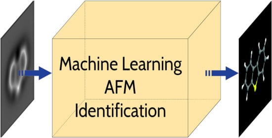
A Deep Learning Approach for Molecular Classification Based on AFM Images


Abstract
:
1. Introduction
2. Materials and Methods
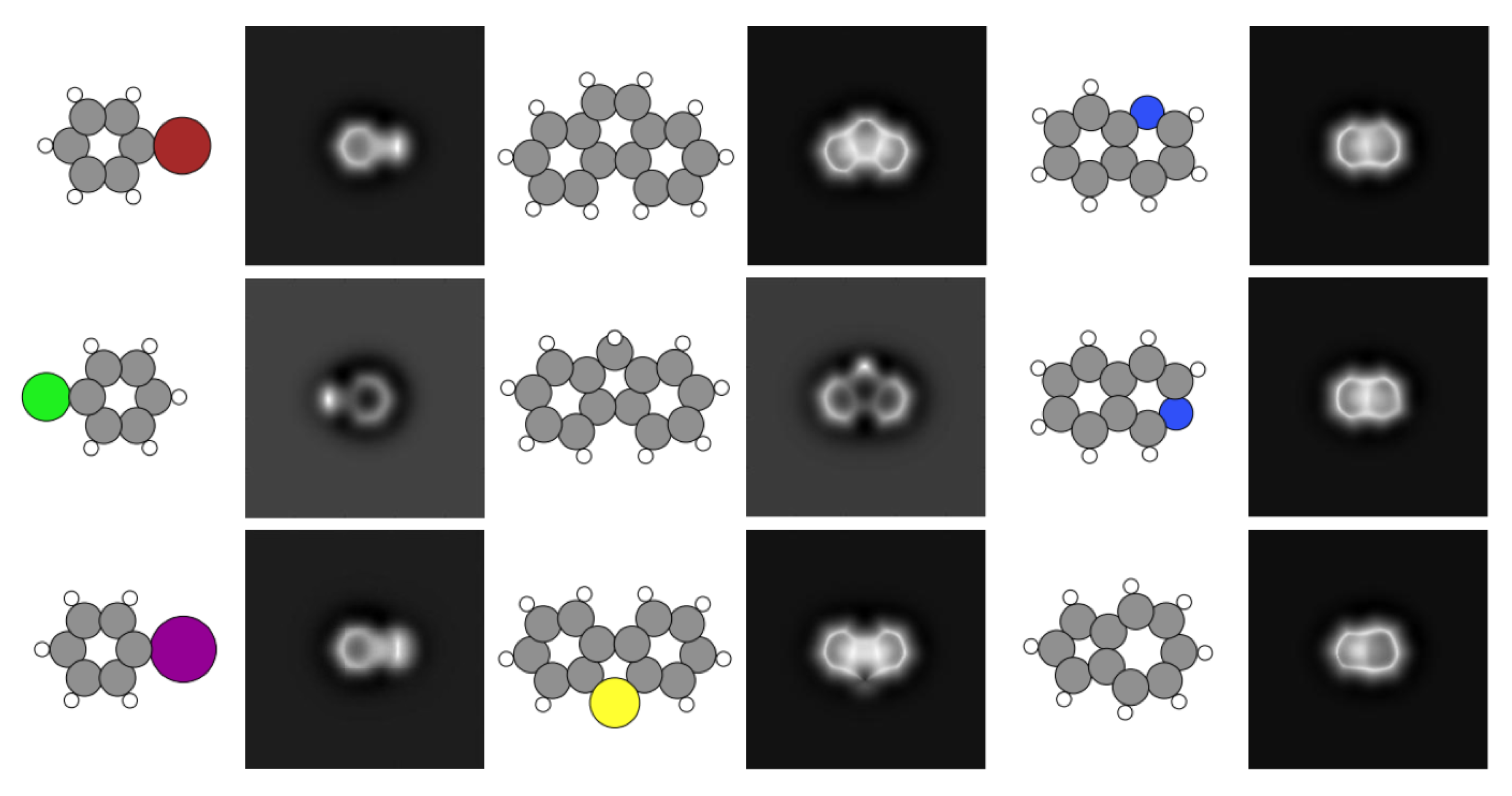
2.1. The SPMTH-60 Dataset of AFM Images
2.2. Molecular Orientations and Operation Parameters for AFM Simulations
2.3. AFM Simulations with the Approximate Version of the FDBM Model Implemented in the PPM Suite of Codes
2.4. First-Principles Calculations
3. Results and Discussion
3.1. Standard Deep-Learning Models for Image Classification
3.1.1. MobileNetV2
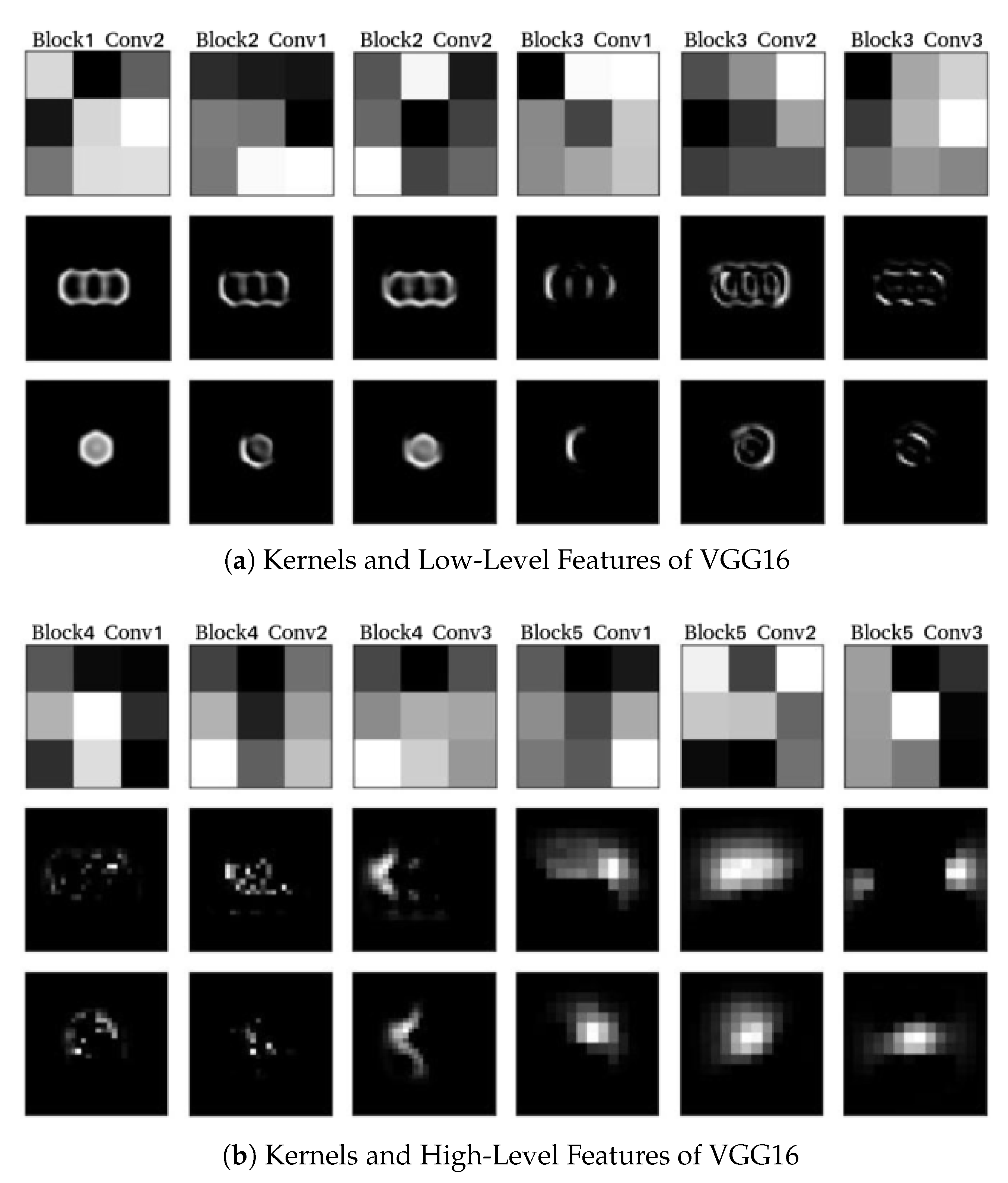
3.1.2. VGG16
3.2. Our ML-AFM Model
3.3. A Variational Autoencoder (VAE) to Improve the Classification of Experimental AFM Images
4. Conclusions
Author Contributions
Funding
Institutional Review Board Statement
Informed Consent Statement
Data Availability Statement
Acknowledgments
Conflicts of Interest
Abbreviations
| (NC)AFM | (non-contact) Atomic Force Microscopy |
| PPM | Probe Particle Model |
| FDBM | Full Density Based Model |
| VASP | Vienna Ab initio Simulation Package |
| DFT | Density Functional Theory |
| VAE | Variational Autoencoder |
| IDG | Image Data Generator |
Appendix A. Implementation and Training Details for the Deep Learning Models
Appendix A.1. Image Data Generator

Appendix A.2. MobileNetV2

Appendix A.3. VGG16


Appendix A.4. Our ML–AFM Model

| Input | Operator | Kernel | OC | Stride | KR-L2 | Act | Connected to | |
|---|---|---|---|---|---|---|---|---|
| Block 1 | Input | - | 1 | - | - | - | - | |
| 1 | - | - | Input | |||||
| 31 | - | ReLU | Input | |||||
| - | 32 | - | - | - | , | |||
| Block 2 | 0.2 | 32 | - | - | - | |||
| 32 | - | ReLU | ||||||
| 32 | - | - | ||||||
| 32 | 0.01 | ReLU | ||||||
| - | 64 | - | - | - | , | |||
| Block 3 | 0.2 | 64 | - | - | - | |||
| 64 | 0.01 | ReLU | ||||||
| 64 | 0.02 | ReLU | ||||||
| 64 | - | ReLU | ||||||
| 64 | - | ReLU | ||||||
| 64 | 0.01 | ReLU | ||||||
| 64 | - | - | ||||||
| - | 128 | - | - | - | , | |||
| Block 4 | 0.2 | 128 | - | - | - | |||
| 128 | - | ReLU | ||||||
| 128 | - | - | ||||||
| 128 | 0.01 | ReLU | ||||||
| 128 | 0.01 | ReLU | ||||||
| 128 | ReLU | |||||||
| 128 | 0.01 | ReLU | ||||||
| 128 | - | - | ||||||
| - | 256 | - | - | - | , | |||
| Block 5 | 256 | - | ReLU | |||||
| 0.2 | 256 | - | - | - | ||||
| Flatten | - | 2304 | - | - | - | |||
| 2304 | FC | - | 60 | - | - | Softmax | Flatten |

Appendix A.5. Variational Autoencoder
References
- Binnig, G.; Quate, C.F.; Gerber, C. Atomic force microscope. Phys. Rev. Lett. 1986, 56, 930–933. [Google Scholar] [CrossRef] [PubMed] [Green Version]
- García, R.; Pérez, R. Dynamic atomic force microscopy methods. Surf. Sci. Rep. 2002, 47, 197–301. [Google Scholar] [CrossRef]
- Giessibl, F.J. Advances in atomic force microscopy. Rev. Mod. Phys. 2003, 75, 949. [Google Scholar] [CrossRef] [Green Version]
- Giessibl, F. Atomic resolution of the silicon (111)-(7 × 7) surface by atomic force microscopy. Science 1995, 267, 1–4. [Google Scholar] [CrossRef] [Green Version]
- Giessibl, F.J. Subatomic Features on the Silicon (111)-(7 × 7) Surface Observed by Atomic Force Microscopy. Science 2000, 289, 422–425. [Google Scholar] [CrossRef]
- Lauritsen, J.V.; Foster, A.S.; Olesen, G.H.; Christensen, M.C.; Kühnle, A.; Helveg, S.; Rostrup-Nielsen, J.R.; Clausen, B.S.; Reichling, M.; Besenbacher, F. Chemical identification of point defects and adsorbates on a metal oxide surface by atomic force microscopy. Nanotechnology 2006, 17, 3436–3441. [Google Scholar] [CrossRef] [Green Version]
- Gross, L.; Mohn, F.; Moll, N.; Liljeroth, P.; Meyer, G. The Chemical Structure of a Molecule Resolved by Atomic Force Microscopy. Science 2009, 325, 1110–1114. [Google Scholar] [CrossRef] [Green Version]
- Pavliček, N.; Gross, L. Generation, manipulation and characterization of molecules by atomic force microscopy. Nat. Rev. Chem. 2017, 1, 0005. [Google Scholar] [CrossRef]
- Hanssen, K.Ø.; Schuler, B.; Williams, A.J.; Demissie, T.B.; Hansen, E.; Andersen, J.H.; Svenson, J.; Blinov, K.; Repisky, M.; Mohn, F.; et al. A Combined Atomic Force Microscopy and Computational Approach for the Structural Elucidation of Breitfussin A and B: Highly Modified Halogenated Dipeptides from Thuiaria breitfussi. Angew. Chem. Int. Ed. 2012, 51, 12238–12241. [Google Scholar] [CrossRef]
- de Oteyza, D.G.; Gorman, P.; Chen, Y.C.; Wickenburg, S.; Riss, A.; Mowbray, D.J.; Etkin, G.; Pedramrazi, Z.; Tsai, H.Z.; Rubio, A.; et al. Direct Imaging of Covalent Bond Structure in Single-Molecule Chemical Reactions. Science 2013, 340, 1434–1437. [Google Scholar] [CrossRef] [Green Version]
- Kawai, S.; Haapasilta, V.; Lindner, B.D.; Tahara, K.; Spijker, P.; Buitendijk, J.A.; Pawlak, R.; Meier, T.; Tobe, Y.; Foster, A.S.; et al. Thermal control of sequential on-surface transformation of a hydrocarbon molecule on a copper surface. Nat. Commun. 2016, 7, 12711. [Google Scholar] [CrossRef] [Green Version]
- Kawai, S.; Takahashi, K.; Ito, S.; Pawlak, R.; Meier, T.; Spijker, P.; Canova, F.F.; Tracey, J.; Nozaki, K.; Foster, A.S.; et al. Competing annulene and radialene structures in a single anti-aromatic molecule studied by high-resolution atomic force microscopy. ACS Nano 2017, 11, 8122–8130. [Google Scholar] [CrossRef] [PubMed]
- Schulz, F.; Jacobse, P.H.; Canova, F.F.; van der Lit, J.; Gao, D.Z.; van den Hoogenband, A.; Han, P.; Klein Gebbink, R.J.M.; Moret, M.E.; Joensuu, P.M.; et al. Precursor geometry determines the growth mechanism in graphene nanoribbons. J. Phys. Chem. C 2017, 121, 2896–2904. [Google Scholar] [CrossRef]
- Schuler, B.; Meyer, G.; Peña, D.; Mullins, O.C.; Gross, L. Unraveling the Molecular Structures of Asphaltenes by Atomic Force Microscopy. J. Am. Chem. Soc. 2015, 137, 9870–9876. [Google Scholar] [CrossRef]
- Moll, N.; Gross, L.; Mohn, F.; Curioni, A.; Meyer, G. A simple model of molecular imaging with noncontact atomic force microscopy. New J. Phys. 2012, 14, 83023. [Google Scholar] [CrossRef]
- Hapala, P.; Kichin, G.; Wagner, C.; Tautz, F.S.; Temirov, R.; Jelínek, P. Mechanism of high-resolution STM/AFM imaging with functionalized tips. Phys. Rev. B 2014, 90, 085421. [Google Scholar] [CrossRef] [Green Version]
- Guo, C.S.; Van Hove, M.A.; Ren, X.; Zhao, Y. High-Resolution Model for Noncontact Atomic Force Microscopy with a Flexible Molecule on the Tip Apex. J. Phys. Chem. C 2015, 119, 1483–1488. [Google Scholar] [CrossRef] [Green Version]
- Sakai, Y.; Lee, A.J.; Chelikowsky, J.R. First-Principles Atomic Force Microscopy Image Simulations with Density Embedding Theory. Nano Lett. 2016, 16, 3242–3246. [Google Scholar] [CrossRef] [PubMed]
- Ellner, M.; Pavliček, N.; Pou, P.; Schuler, B.; Moll, N.; Meyer, G.; Gross, L.; Pérez, R. The Electric Field of CO Tips and Its Relevance for Atomic Force Microscopy. Nano Lett. 2016, 16, 1974–1980. [Google Scholar] [CrossRef]
- Van Der Lit, J.; Di Cicco, F.; Hapala, P.; Jelínek, P.; Swart, I. Submolecular Resolution Imaging of Molecules by Atomic Force Microscopy: The Influence of the Electrostatic Force. Phys. Rev. Lett. 2016, 116, 096102. [Google Scholar] [CrossRef] [PubMed]
- Hapala, P.; Švec, M.; Stetsovych, O.; van der Heijden, N.J.; Ondráček, M.; van der Lit, J.; Mutombo, P.; Swart, I.; Jelínek, P. Mapping the electrostatic force field of single molecules from high-resolution scanning probe images. Nat. Commun. 2016, 7, 11560. [Google Scholar] [CrossRef]
- Ellner, M.; Pou, P.; Pérez, R. Atomic force microscopy contrast with CO functionalized tips in hydrogen-bonded molecular layers: Does the real tip charge distribution play a role? Phys. Rev. B 2017, 96, 075418. [Google Scholar] [CrossRef] [Green Version]
- Ellner, M.; Pou, P.; Peérez, R. Molecular identification, bond order discrimination, and apparent intermolecular features in atomic force microscopy studied with a charge density based method. ACS Nano 2019, 13, 786–795. [Google Scholar] [CrossRef]
- Lin, T.Y.; Maire, M.; Belongie, S.; Hays, J.; Perona, P.; Ramanan, D.; Dollár, P.; Zitnick, C.L. Microsoft COCO: Common objects in context. In Proceedings of the European Conference on Computer Vision (ECCV), Zurich, Switzerland, 6–12 September 2014; Springer: Berlin/Heidelberg, Germany, 2014; pp. 740–755. [Google Scholar]
- Goyal, Y.; Khot, T.; Agrawal, A.; Summers-Stay, D.; Batra, D.; Parikh, D. Making the V in VQA Matter: Elevating the Role of Image Understanding in Visual Question Answering. Int. J. Comput. Vis. 2019, 127, 398–414. [Google Scholar] [CrossRef] [Green Version]
- Antol, S.; Agrawal, A.; Lu, J.; Mitchell, M.; Batra, D.; Lawrence Zitnick, C.; Parikh, D. VQA: Visual Question Answering. In Proceedings of the 2015 IEEE International Conference on Computer Vision (ICCV), Santiago, Chile, 7–13 December 2015. [Google Scholar]
- Netzer, Y.; Wang, T.; Coates, A.; Bissacco, A.; Wu, B.; Ng, A.Y. Reading Digits in Natural Images with Unsupervised Feature Learning 2011. In Proceedings of the NIPS Workshop, Granada, Spain, 16–17 December 2011. [Google Scholar]
- Cui, H.; Zhang, H.; Ganger, G.R.; Gibbons, P.B.; Xing, E.P. GeePS: Scalable Deep Learning on Distributed GPUs with a GPU-Specialized Parameter Server. In Proceedings of the Eleventh European Conference on Computer Systems (EuroSys ’16), London, UK, 18–21 April 2016. [Google Scholar]
- Jia, Y.; Shelhamer, E.; Donahue, J.; Karayev, S.; Long, J.; Girshick, R.; Guadarrama, S.; Darrell, T. Caffe: Convolutional Architecture for Fast Feature Embedding. In Proceedings of the 22nd ACM international conference on Multimedia (MM ’14), Orlando, FL, USA, 3–7 November 2014; pp. 675–678. [Google Scholar]
- Abadi, M.; Barham, P.; Chen, J.; Chen, Z.; Davis, A.; Dean, J.; Devin, M.; Ghemawat, S.; Irving, G.; Isard, M.; et al. TensorFlow: A system for large-scale machine learning. arXiv 2016, arXiv:1605.08695. [Google Scholar]
- Paszke, A.; Gross, S.; Chintala, S.; Chanan, G.; Yang, E.; DeVito, Z.; Lin, Z.; Desmaison, A.; Antiga, L.; Lerer, A. Automatic differentiation in pytorch. In Proceedings of the NIPS Workshop 2017, Long Beach, CA, USA, 4–9 December 2017. [Google Scholar]
- Lawrence, S.; Giles, C.L.; Tsoi, A.C.; Back, A.D. Face recognition: A convolutional neural-network approach. IEEE Trans. Neural Netw. 1997, 8, 98–113. [Google Scholar] [CrossRef] [Green Version]
- Sainath, T.N.; Mohamed, A.r.; Kingsbury, B.; Ramabhadran, B. Deep convolutional neural networks for LVCSR. In Proceedings of the 2013 IEEE International Conference on Acoustics, Speech and Signal Processing, Vancouver, BC, Canada, 26–31 May 2013; pp. 8614–8618. [Google Scholar]
- Simard, P.Y.; Steinkraus, D.; Platt, J.C. Best practices for convolutional neural networks applied to visual document analysis. In Proceedings of the Seventh International Conference on Document Analysis and Recognition, Edinburgh, UK, 3–6 August 2003; pp. 958–963. [Google Scholar]
- Krizhevsky, A.; Sutskever, I.; Hinton, G.E. ImageNet Classification with Deep Convolutional Neural Networks. In 25 NIPS Workshop; Curran Associates, Inc.: Kingsbury, NV, USA, 2012; pp. 1097–1105. [Google Scholar]
- Shen, D.; Wu, G.; Suk, H.I. Deep learning in medical image analysis. Annu. Rev. Biomed. Eng. 2017, 19, 221–248. [Google Scholar] [CrossRef] [Green Version]
- Gheisari, M.; Wang, G.; Bhuiyan, M.Z.A. A survey on deep learning in big data. In Proceedings of the IEEE International Conference on Computational Science and Engineering (CSE) and IEEE International Conference on Embedded and Ubiquitous Computing (EUC), Guangzhou, China, 21–24 July 2017; Volume 2, pp. 173–180. [Google Scholar]
- Rao, M.R.N.; Prasad, V.V.; Teja, P.S.; Zindavali, M.; Reddy, O.P. A Survey on Prevention of Overfitting in Convolution Neural Networks Using Machine Learning Techniques. Int. J. Eng. Technol. 2018, 7, 177–180. [Google Scholar]
- Neyshabur, B.; Bhojanapalli, S.; McAllester, D.; Srebro, N. Exploring generalization in deep learning. In Proceedings of the Advances in Neural Information Processing Systems 30 (NIPS 2017), Long Beach, CA, USA, 4–9 December 2017; pp. 5947–5956. [Google Scholar]
- Hawkins, D.M. The Problem of Overfitting. J. Chem. Inf. Comput. Sci. 2004, 44, 1–12. [Google Scholar] [CrossRef] [PubMed]
- Srivastava, N.; Hinton, G.; Krizhevsky, A.; Sutskever, I.; Salakhutdinov, R. Dropout: A Simple Way to Prevent Neural Networks from Overfitting. J. Mach. Learn. Res. 2014, 15, 1929–1958. [Google Scholar]
- Cogswell, M.; Ahmed, F.; Girshick, R.; Zitnick, L.; Batra, D. Reducing overfitting in deep networks by decorrelating representations. arXiv 2015, arXiv:1511.06068. [Google Scholar]
- Alldritt, B.; Hapala, P.; Oinonen, N.; Urtev, F.; Krejci, O.; Canova, F.F.; Kannala, J.; Schulz, F.; Liljeroth, P.; Foster, A.S. Automated structure discovery in atomic force microscopy. Sci. Adv. 2020, 6, eaay6913. [Google Scholar] [CrossRef] [Green Version]
- Sugimoto, Y.; Pou, P.; Abe, M.; Jelínek, P.; Pérez, R.; Morita, S.; Custance, Ó. Chemical identification of individual surface atoms by atomic force microscopy. Nature 2007, 446, 64. [Google Scholar] [CrossRef] [PubMed] [Green Version]
- Sandler, M.; Howard, A.; Zhu, M.; Zhmoginov, A.; Chen, L.C. Mobilenetv2: Inverted residuals and linear bottlenecks. In Proceedings of the 2018 IEEE/CVF Conference on Computer Vision and Pattern Recognition, Salt Lake City, UT, USA, 18–23 June 2018; pp. 4510–4520. [Google Scholar]
- Simonyan, K.; Zisserman, A. Very deep convolutional networks for large-scale image recognition. arXiv 2014, arXiv:1409.1556. [Google Scholar]
- Zahl, P.; Zhang, Y. Guide for Atomic Force Microscopy Image Analysis To Discriminate Heteroatoms in Aromatic Molecules. Energy Fuels 2019, 33, 4775–4780. [Google Scholar] [CrossRef] [Green Version]
- Kingma, D.P.; Welling, M. Auto-encoding variational bayes. arXiv 2013, arXiv:1312.6114. [Google Scholar]
- Dilokthanakul, N.; Mediano, P.A.; Garnelo, M.; Lee, M.C.; Salimbeni, H.; Arulkumaran, K.; Shanahan, M. Deep unsupervised clustering with gaussian mixture variational autoencoders. arXiv 2016, arXiv:1611.02648. [Google Scholar]
- Kim, S.; Thiessen, P.A.; Bolton, E.E.; Chen, J.; Fu, G.; Gindulyte, A.; Han, L.; He, J.; He, S.; Shoemaker, B.A.; et al. PubChem substance and compound databases. Nucleic Acids Res. 2016, 44, D1202–D1213. [Google Scholar] [CrossRef]
- Liebig, A.; Hapala, P.; Weymouth, A.J.; Giessibl, F.J. Quantifying the evolution of atomic interaction of a complex surface with a functionalized atomic force microscopy tip. Sci. Rep. 2020, 10, 14104. [Google Scholar] [CrossRef]
- Hapala, P.; Temirov, R.; Tautz, F.S.; Jelínek, P. Origin of High-Resolution IETS-STM Images of Organic Molecules with Functionalized Tips. Phys. Rev. Lett. 2014, 113, 226101. [Google Scholar] [CrossRef] [Green Version]
- Unpublished images courtesy of Dr. Percy Zahl (Brookhaven National Laboratory, Brookhaven, NY, USA) and Dr. Yunlong Zhang (ExxonMobil Research and Engineering, Annandale, NJ, USA).
- Kresse, G.; Furthmüller, J. Efficiency of ab-initio total energy calculations for metals and semiconductors using a plane-wave basis set. Comput. Mater. Sci. 1996, 6, 15–50. [Google Scholar] [CrossRef]
- Kresse, G.; Furthmüller, J. Efficient iterative schemes for ab initio total-energy calculations using a plane-wave basis set. Phys. Rev. B 1996, 54, 11169. [Google Scholar] [CrossRef]
- Blöchl, P.E. Projector augmented-wave method. Phys. Rev. B 1994, 50, 17953. [Google Scholar] [CrossRef] [Green Version]
- Kresse, G.; Joubert, D. From ultrasoft pseudopotentials to the projector augmented-wave method. Phys. Rev. B 1999, 59, 1758. [Google Scholar] [CrossRef]
- Perdew, J.P.; Burke, K.; Ernzerhof, M. Generalized Gradient Approximation Made Simple. Phys. Rev. Lett. 1996, 77, 3865–3868. [Google Scholar] [CrossRef] [Green Version]
- Grimme, S.; Antony, J.; Ehrlich, S.; Krieg, H. A consistent and accurate ab initio parametrization of density functional dispersion correction (DFT-D) for the 94 elements H-Pu. J. Chem. Phys. 2010, 132, 154104. [Google Scholar] [CrossRef] [PubMed] [Green Version]
- Chollet, F. Deep Learning with Python; Manning Publications Co.: Shelter Island, NY, USA, 2018. [Google Scholar]
- Prechelt, L. Early stopping-but when? In Neural Networks: Tricks of the Trade; Springer: Berlin/Heidelberg, Germany, 1998; pp. 55–69. [Google Scholar]
- Kingma, D.P.; Ba, J. Adam: A method for stochastic optimization. arXiv 2014, arXiv:1412.6980. [Google Scholar]
- Vincent, P.; Larochelle, H.; Bengio, Y.; Manzagol, P.A. Extracting and composing robust features with denoising autoencoders. In Proceedings of the 25th International Conference on Machine Learning (ICML ’08), Helsinki, Finland, 5–9 July 2008; pp. 1096–1103. [Google Scholar]
- Iglovikov, V.; Shvets, A. Ternausnet: U-net with vgg11 encoder pre-trained on imagenet for image segmentation. arXiv 2018, arXiv:1801.05746. [Google Scholar]
- Liu, G.; Reda, F.A.; Shih, K.J.; Wang, T.C.; Tao, A.; Catanzaro, B. Image inpainting for irregular holes using partial convolutions. In Proceedings of the ECCV, Munich, Germany, 8–14 September 2018; pp. 85–100. [Google Scholar]
- Jorge, J.; Vieco, J.; Paredes, R.; Sánchez, J.A.; Benedí, J.M. Empirical Evaluation of Variational Autoencoders for Data Augmentation. In Proceedings of the 13th International Joint Conference on Computer Vision, Imaging and Computer Graphics Theory and Applications—Volume 5: VISAPP, INSTICC, Madeira, Portugal, 27–29 January 2018; SciTePress: Madeira, Portugal, 2018; pp. 96–104. [Google Scholar]
- Chollet, F. Keras: The Python Deep Learning Library. Astrophysics Source Code Library; 2018, ascl:1806.022. Available online: https://ascl.net/.
- Russakovsky, O.; Deng, J.; Su, H.; Krause, J.; Satheesh, S.; Ma, S.; Huang, Z.; Karpathy, A.; Khosla, A.; Bernstein, M. Imagenet large scale visual recognition challenge. Int. J. Comput. Vis. 2015, 115, 211–252. [Google Scholar] [CrossRef] [Green Version]
- Glorot, X.; Bordes, A.; Bengio, Y. Deep sparse rectifier neural networks. In Proceedings of the Machine Learning Research, Fort Lauderdale, FL, USA, 11–13 April 2011; Volume 15, pp. 315–323. [Google Scholar]
- Ruder, S. An overview of gradient descent optimization algorithms. arXiv 2016, arXiv:1609.04747. [Google Scholar]


| Simulations | VAE | ||||||
|---|---|---|---|---|---|---|---|
| Molecule | Support | MNtV2 | VGG16 | MLAFM | MNtV2 | VGG16 | MLAFM |
| ACR | 68 | 0.06 | 0.08 | 0.82 | 0.80 | 0.82 | 0.96 |
| CAR | 11 | 0.00 | 0.00 | 0.45 | 0.45 | 0.72 | 0.72 |
| DIB | 31 | 0.00 | 0.00 | 0.62 | 0.19 | 0.74 | 0.90 |
Publisher’s Note: MDPI stays neutral with regard to jurisdictional claims in published maps and institutional affiliations. |
© 2021 by the authors. Licensee MDPI, Basel, Switzerland. This article is an open access article distributed under the terms and conditions of the Creative Commons Attribution (CC BY) license (https://creativecommons.org/licenses/by/4.0/).
Share and Cite
Carracedo-Cosme, J.; Romero-Muñiz, C.; Pérez, R. A Deep Learning Approach for Molecular Classification Based on AFM Images. Nanomaterials 2021, 11, 1658. https://doi.org/10.3390/nano11071658
Carracedo-Cosme J, Romero-Muñiz C, Pérez R. A Deep Learning Approach for Molecular Classification Based on AFM Images. Nanomaterials. 2021; 11(7):1658. https://doi.org/10.3390/nano11071658
Chicago/Turabian StyleCarracedo-Cosme, Jaime, Carlos Romero-Muñiz, and Rubén Pérez. 2021. "A Deep Learning Approach for Molecular Classification Based on AFM Images" Nanomaterials 11, no. 7: 1658. https://doi.org/10.3390/nano11071658