Practices and Trends of Machine Learning Application in Nanotoxicology

 ,
,
Abstract
:
1. Introduction
2. Methods
2.1. Search Design
2.2. Eligibility and Exclusion Criteria
2.3. Analysis
3. Results
3.1. Dataset Formation
3.2. Data Pre-Processing
3.2.1. Feature Reduction
3.2.2. Feature Selection
3.2.3. Pre-Processing Techniques
3.2.4. Normalization and Discretization
3.2.5. Class Balancing
3.2.6. Missing Values
3.2.7. Molecular Structures’ Codification
3.2.8. Data Splitting
3.3. Model Implementation
3.4. Model Validation and Applicability Domain
3.4.1. Goodness-of-Fit
3.4.2. Robustness
3.4.3. Chance Testing
3.4.4. Predictability
3.4.5. Ranking of Classifiers
3.4.6. Applicability Domain (AD)
4. Discussion
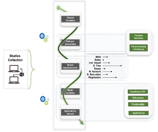
4.1. The Framework
4.2. The Algorithms
4.3. Challenges and Perspectives
5. Conclusions
- a variety of ML algorithms have been used during the last decade with non-linear modelling gaining popularity;
- linear regression is still a popular method, enriched with nonlinear techniques;
- there is a clear shift from theoretical descriptors and traditional QSAR modelling to models incorporating nano-specific features, even though there is limited consensus on which features must be considered;
- there is great diversity in data pre-processing techniques depending on datasets and the ML algorithm chosen;
- there is little technical convergence in pre-modelling stage methods compared to model implementation and validation;
- there is, in general, a lack of justification of model selection. There is also little justification on the validation metrics choice.
Supplementary Materials
Author Contributions
Funding
Conflicts of Interest
References
- Chen, R.; Qiao, J.; Bai, R.; Zhao, Y.; Chen, C. Intelligent testing strategy and analytical techniques for the safety assessment of nanomaterials. Anal. Bioanal. Chem. 2018, 410, 6051–6066. [Google Scholar] [CrossRef] [PubMed]
- Schwarz-Plaschg, C.; Kallhoff, A.; Eisenberger, I. Making Nanomaterials Safer by Design. NanoEthics 2017, 11, 277–281. [Google Scholar] [CrossRef] [Green Version]
- Kraegeloh, A.; Suarez-Merino, B.; Sluijters, T.; Micheletti, C. Implementation of Safe-by-Design for Nanomaterial Development and Safe Innovation: Why We Need a Comprehensive Approach. Nanomaterials 2018, 8, 239. [Google Scholar] [CrossRef] [PubMed] [Green Version]
- Puzyn, T.; Jeliazkova, N.; Sarimveis, H.; Marchese Robinson, R.L.; Lobaskin, V.; Rallo, R.; Richarz, A.-N.; Gajewicz, A.; Papadopulos, M.G.; Hastings, J.; et al. Perspectives from the NanoSafety Modelling Cluster on the validation criteria for (Q)SAR models used in nanotechnology. Food Chem. Toxicol. 2018, 112, 478–494. [Google Scholar] [CrossRef] [PubMed]
- Haase, A.; Klaessig, F. EU US Roadmap Nanoinformatics 2030; EU NanoSafety Cluster: Copenhagen, Denmark, 2018. [Google Scholar]
- Burgdorf, T.; Piersma, A.H.; Landsiedel, R.; Clewell, R.; Kleinstreuer, N.; Oelgeschläger, M.; Desprez, B.; Kienhuis, A.; Bos, P.; de Vries, R.; et al. Workshop on the validation and regulatory acceptance of innovative 3R approaches in regulatory toxicology—Evolution versus revolution. Toxicol. In Vitro 2019, 59, 1–11. [Google Scholar] [CrossRef] [Green Version]
- ECHA. Non-Animal Approaches—Current Status of Regulatory Applicability under the REACH, CLP and Biocidal Products Regulations; ECHA: Helsinki, Finland, 2017; p. 163. [Google Scholar]
- Villaverde, J.J.; Sevilla-Morán, B.; López-Goti, C.; Alonso-Prados, J.L.; Sandín-España, P. Considerations of nano-QSAR/QSPR models for nanopesticide risk assessment within the European legislative framework. Sci. Total Environ. 2018, 634, 1530–1539. [Google Scholar] [CrossRef]
- Quik, J.T.K.; Bakker, M.; van de Meent, D.; Poikkimäki, M.; Dal Maso, M.; Peijnenburg, W. Directions in QPPR development to complement the predictive models used in risk assessment of nanomaterials. NanoImpact 2018, 11, 58–66. [Google Scholar] [CrossRef]
- Lamon, L.; Asturiol, D.; Richarz, A.; Joossens, E.; Graepel, R.; Aschberger, K.; Worth, A. Grouping of nanomaterials to read-across hazard endpoints: From data collection to assessment of the grouping hypothesis by application of chemoinformatic techniques. Part. Fibre Toxicol. 2018, 15, 37. [Google Scholar] [CrossRef]
- Lamon, L.; Aschberger, K.; Asturiol, D.; Richarz, A.; Worth, A. Grouping of nanomaterials to read-across hazard endpoints: A review. Nanotoxicology 2018. [Google Scholar] [CrossRef]
- Giusti, A.; Atluri, R.; Tsekovska, R.; Gajewicz, A.; Apostolova, M.D.; Battistelli, C.L.; Bleeker, E.A.J.; Bossa, C.; Bouillard, J.; Dusinska, M.; et al. Nanomaterial grouping: Existing approaches and future recommendations. NanoImpact 2019, 16, 100182. [Google Scholar] [CrossRef]
- OECD. OECD. Guidance Document on the Validation of (Quantitative) Structure-Activity Relationship [(Q)SAR] Models; OECD: Paris, France, 2014. [Google Scholar] [CrossRef]
- Basei, G.; Hristozov, D.; Lamon, L.; Zabeo, A.; Jeliazkova, N.; Tsiliki, G.; Marcomini, A.; Torsello, A. Making use of available and emerging data to predict the hazards of engineered nanomaterials by means of in silico tools: A critical review. NanoImpact 2019, 13, 76–99. [Google Scholar] [CrossRef]
- Worth, A.A.K.; Asturiol, B.D.; Bessems, J.; Gerloff, K.B.; Graepel, R.; Joossens, E.; Lamon, L.; Palosaari, T.; Richarz, A. Evaluation of the Availability and Applicability of Computational Approaches in the Safety Assessment of Nanomaterials; Final Report of the Nanocomput Project; JRC: Ispra, Italy, 2017. [Google Scholar]
- Lamon, L.; Asturiol, D.; Vilchez, A.; Ruperez-Illescas, R.; Cabellos, J.; Richarz, A.; Worth, A. Computational models for the assessment of manufactured nanomaterials: Development of model reporting standards and mapping of the model landscape. Comput. Toxicol. 2019, 9, 143–151. [Google Scholar] [CrossRef] [PubMed]
- Schneider, K.; Schwarz, M.; Burkholder, I.; Kopp-Schneider, A.; Edler, L.; Kinsner-Ovaskainen, A.; Hartung, T.; Hoffmann, S. “ToxRTool”, a new tool to assess the reliability of toxicological data. Toxicol. Lett. 2009, 189, 138–144. [Google Scholar] [CrossRef] [PubMed]
- Furxhi, I.; Murphy, F.; Mullins, M.; Arvanitis, A.; Poland, A.C. Nanotoxicology data for in silico tools. A literature review. Nanotoxicology 2020, submitted. [Google Scholar]
- OECD. Guidance Document on the Validation of (Quantitative) Structure-Activity Relationships [(Q)SAR] Models; OECD: Paris, France, 2007; pp. 1–154. [Google Scholar]
- Li, M.; Zou, P.; Tyner, K.; Lee, S. Physiologically Based Pharmacokinetic (PBPK) Modeling of Pharmaceutical Nanoparticles. AAPS J. 2017, 19, 26–42. [Google Scholar] [CrossRef]
- Yuan, D.; He, H.; Wu, Y.; Fan, J.; Cao, Y. Physiologically Based Pharmacokinetic Modeling of Nanoparticles. J. Pharm. Sci. 2019, 108, 58–72. [Google Scholar] [CrossRef] [Green Version]
- Danauskas, S.M.; Jurs, P.C. Prediction of C60 Solubilities from Solvent Molecular Structures. J. Chem. Inf. Comput. Sci. 2001, 41, 419–424. [Google Scholar] [CrossRef]
- Pourbasheer, E.; Aalizadeh, R.; Ardabili, J.S.; Ganjali, M.R. QSPR study on solubility of some fullerenes derivatives using the genetic algorithms—Multiple linear regression. J. Mol. Liq. 2015, 204, 162–169. [Google Scholar] [CrossRef]
- Bouwmeester, H.; Poortman, J.; Peters, R.J.; Wijma, E.; Kramer, E.; Makama, S.; Puspitaninganindita, K.; Marvin, H.J.; Peijnenburg, A.A.; Hendriksen, P.J. Characterization of Translocation of Silver Nanoparticles and Effects on Whole-Genome Gene Expression Using an In Vitro Intestinal Epithelium Coculture Model. ACS Nano 2011, 5, 4091–4103. [Google Scholar] [CrossRef]
- Basant, N.; Gupta, S. Multi-target QSTR modeling for simultaneous prediction of multiple toxicity endpoints of nano-metal oxides. Nanotoxicology 2017, 11, 339–350. [Google Scholar] [CrossRef]
- Salahinejad, M.; Zolfonoun, E. QSAR studies of the dispersion of SWNTs in different organic solvents. J. Nanopart. Res. 2013, 15, 2028. [Google Scholar] [CrossRef]
- Petrova, T.; Rasulev, B.F.; Toropov, A.A.; Leszczynska, D.; Leszczynski, J. Improved model for fullerene C60 solubility in organic solvents based on quantum-chemical and topological descriptors. J. Nanopart. Res. 2011, 13, 3235–3247. [Google Scholar] [CrossRef]
- Papa, E.; Doucet, J.P.; Doucet-Panaye, A. Linear and non-linear modelling of the cytotoxicity of TiO2 and ZnO nanoparticles by empirical descriptors. SAR QSAR Environ. Res. 2015, 26, 647–665. [Google Scholar] [CrossRef] [PubMed]
- Oksel, C.; Ma, C.Y.; Liu, J.J.; Wilkins, T.; Wang, X.Z. (Q)SAR modelling of nanomaterial toxicity: A critical review. Particuology 2015, 21, 1–19. [Google Scholar] [CrossRef]
- Oksel, C.; Winkler, D.A.; Ma, C.Y.; Wilkins, T.; Wang, X.Z. Accurate and interpretable nanoSAR models from genetic programming-based decision tree construction approaches. Nanotoxicology 2016, 10, 1001–1012. [Google Scholar] [CrossRef]
- Mikolajczyk, A.; Gajewicz, A.; Mulkiewicz, E.; Rasulev, B.; Marchelek, M.; Diak, M.; Hirano, S.; Zaleska-Medynska, A.; Puzyn, T. Nano-QSAR modeling for ecosafe design of heterogeneous TiO2-based nano-photocatalysts. Environ. Sci. Nano 2018, 5, 1150–1160. [Google Scholar] [CrossRef]
- Shao, C.-Y.; Chen, S.-Z.; Su, B.-H.; Tseng, Y.J.; Esposito, E.X.; Hopfinger, A.J. Dependence of QSAR Models on the Selection of Trial Descriptor Sets: A Demonstration Using Nanotoxicity Endpoints of Decorated Nanotubes. J. Chem. Inf. Model. 2013, 53, 142–158. [Google Scholar] [CrossRef]
- Wen, D.; Shan, X.; He, G.; Chen, H. Prediction for cellular uptake of manufactured nanoparticles to pancreatic cancer cells. Revue Roumaine Chimie 2015, 60, 367–370. [Google Scholar]
- Gajewicz, A.; Schaeublin, N.; Rasulev, B.; Hussain, S.; Leszczynska, D.; Puzyn, T.; Leszczynski, J. Towards understanding mechanisms governing cytotoxicity of metal oxides nanoparticles: Hints from nano-QSAR studies. Nanotoxicology 2015, 9, 313–325. [Google Scholar] [CrossRef]
- Puzyn, T.; Rasulev, B.; Gajewicz, A.; Hu, X.; Dasari, T.P.; Michalkova, A.; Hwang, H.-M.; Toropov, A.; Leszczynska, D.; Leszczynski, J. Using nano-QSAR to predict the cytotoxicity of metal oxide nanoparticles. Nat. Nanotechnol. 2011, 6, 175. [Google Scholar] [CrossRef]
- Helma, C.; Rautenberg, M.; Gebele, D. Nano-Lazar: Read across Predictions for Nanoparticle Toxicities with Calculated and Measured Properties. Front. Pharmacol. 2017, 8. [Google Scholar] [CrossRef] [Green Version]
- Trinh, T.X.; Choi, J.S.; Jeon, H.; Byun, H.G.; Yoon, T.H.; Kim, J. Quasi-SMILES-Based Nano-Quantitative Structure-Activity Relationship Model to Predict the Cytotoxicity of Multiwalled Carbon Nanotubes to Human Lung Cells. Chem. Res. Toxicol. 2018, 31, 183–190. [Google Scholar] [CrossRef] [PubMed]
- Bigdeli, A.; Hormozi-Nezhad, M.R.; Parastar, H. Using nano-QSAR to determine the most responsible factor(s) in gold nanoparticle exocytosis. RSC Adv. 2015, 5, 57030–57037. [Google Scholar] [CrossRef]
- Oksel, C.; Ma, C.Y.; Wang, X.Z. Structure-activity Relationship Models for Hazard Assessment and Risk Management of Engineered Nanomaterials. Procedia Eng. 2015, 102, 1500–1510. [Google Scholar] [CrossRef] [Green Version]
- Papa, E.; Doucet, J.P.; Sangion, A.; Doucet-Panaye, A. Investigation of the influence of protein corona composition on gold nanoparticle bioactivity using machine learning approaches. SAR QSAR Environ. Res. 2016, 27, 521–538. [Google Scholar] [CrossRef] [PubMed]
- Mu, Y.; Wu, F.; Zhao, Q.; Ji, R.; Qie, Y.; Zhou, Y.; Hu, Y.; Pang, C.; Hristozov, D.; Giesy, J.P.; et al. Predicting toxic potencies of metal oxide nanoparticles by means of nano-QSARs. Nanotoxicology 2016, 10, 1207–1214. [Google Scholar] [CrossRef] [PubMed]
- Ghaedi, M.; Ghaedi, A.M.; Hossainpour, M.; Ansari, A.; Habibi, M.H.; Asghari, A.R. Least square-support vector (LS-SVM) method for modeling of methylene blue dye adsorption using copper oxide loaded on activated carbon: Kinetic and isotherm study. J. Ind. Eng. Chem. 2014, 20, 1641–1649. [Google Scholar] [CrossRef]
- Jha, S.K.; Yoon, T.H.; Pan, Z. Multivariate statistical analysis for selecting optimal descriptors in the toxicity modeling of nanomaterials. Comput. Biol. Med. 2018, 99, 161–172. [Google Scholar] [PubMed]
- Borders, T.L.; Fonseca, A.F.; Zhang, H.; Cho, K.; Rusinko, A. Developing Descriptors to Predict Mechanical Properties of Nanotubes. J. Chem. Inf. Model. 2013, 53, 773–782. [Google Scholar] [CrossRef]
- Bygd, H.C.; Forsmark, K.D.; Bratlie, K.M. Altering in vivo macrophage responses with modified polymer properties. Biomaterials 2015, 56, 187–197. [Google Scholar] [CrossRef]
- Kar, S.; Gajewicz, A.; Puzyn, T.; Roy, K. Nano-quantitative structure–activity relationship modeling using easily computable and interpretable descriptors for uptake of magnetofluorescent engineered nanoparticles in pancreatic cancer cells. Toxicol. In Vitro 2014, 28, 600–606. [Google Scholar] [CrossRef] [PubMed]
- Walkey, C.D.; Olsen, J.B.; Song, F.; Liu, R.; Guo, H.; Olsen, D.W.H.; Cohen, Y.; Emili, A.; Chan, W.C.W. Protein Corona Fingerprinting Predicts the Cellular Interaction of Gold and Silver Nanoparticles. ACS Nano 2014, 8, 2439–2455. [Google Scholar] [CrossRef] [PubMed]
- Rofouei, M.K.; Salahinejad, M.; Ghasemi, J.B. An Alignment Independent 3D-QSAR Modeling of Dispersibility of Single-walled Carbon Nanotubes in Different Organic Solvents. Fuller. Nanotub. Carbon Nanostruct. 2014, 22, 605–617. [Google Scholar] [CrossRef]
- Rong, L.; Robert, R.; Muhammad, B.; Yoram, C. Quantitative Structure-Activity Relationships for Cellular Uptake of Surface-Modified Nanoparticles. In Combinatorial Chemistry & High Throughput Screening; Bentham Science: Bussum, The Netherlands, 2015; Volume 18, pp. 365–375. [Google Scholar]
- Liu, R.; Jiang, W.; Walkey, C.D.; Chan, W.C.W.; Cohen, Y. Prediction of nanoparticles-cell association based on corona proteins and physicochemical properties. Nanoscale 2015, 7, 9664–9675. [Google Scholar] [CrossRef]
- Luan, F.; Kleandrova, V.V.; González-Díaz, H.; Ruso, J.M.; Melo, A.; Speck-Planche, A.; Cordeiro, M.N.D.S. Computer-aided nanotoxicology: Assessing cytotoxicity of nanoparticles under diverse experimental conditions by using a novel QSTR-perturbation approach. Nanoscale 2014, 6, 10623–10630. [Google Scholar] [CrossRef]
- Speck-Planche, A.; Kleandrova, V.V.; Luan, F.; Cordeiro, M.N. Computational modeling in nanomedicine: Prediction of multiple antibacterial profiles of nanoparticles using a quantitative structure-activity relationship perturbation model. Nanomedicine 2015, 10, 193–204. [Google Scholar] [CrossRef]
- Kar, S.; Gajewicz, A.; Roy, K.; Leszczynski, J.; Puzyn, T. Extrapolating between toxicity endpoints of metal oxide nanoparticles: Predicting toxicity to Escherichia coli and human keratinocyte cell line (HaCaT) with Nano-QTTR. Ecotoxicol. Environ. Saf. 2016, 126, 238–244. [Google Scholar] [CrossRef] [Green Version]
- Yousefinejad, S.; Honarasa, F.; Abbasitabar, F.; Arianezhad, Z. New LSER Model Based on Solvent Empirical Parameters for the Prediction and Description of the Solubility of Buckminsterfullerene in Various Solvents. J. Solut. Chem. 2013, 42, 1620–1632. [Google Scholar] [CrossRef]
- Ghorbanzadeh, M.; Fatemi, M.H.; Karimpour, M. Modeling the Cellular Uptake of Magnetofluorescent Nanoparticles in Pancreatic Cancer Cells: A Quantitative Structure Activity Relationship Study. Ind. Eng. Chem. Res. 2012, 51, 10712–10718. [Google Scholar] [CrossRef]
- Epa, V.C.; Burden, F.R.; Tassa, C.; Weissleder, R.; Shaw, S.; Winkler, D.A. Modeling Biological Activities of Nanoparticles. Nano Lett. 2012, 12, 5808–5812. [Google Scholar] [CrossRef]
- Le, T.C.; Yin, H.; Chen, R.; Chen, Y.; Zhao, L.; Casey, P.S.; Chen, C.; Winkler, D.A. An Experimental and Computational Approach to the Development of ZnO Nanoparticles that are Safe by Design. Small 2016, 12, 3568–3577. [Google Scholar] [CrossRef] [PubMed]
- Winkler, D.A.; Burden, F.R.; Yan, B.; Weissleder, R.; Tassa, C.; Shaw, S.; Epa, V.C. Modelling and predicting the biological effects of nanomaterials. SAR QSAR Environ. Res. 2014, 25, 161–172. [Google Scholar] [CrossRef] [PubMed]
- Bilal, M.; Oh, E.; Liu, R.; Breger, J.C.; Medintz, I.L.; Cohen, Y. Bayesian Network Resource for Meta-Analysis: Cellular Toxicity of Quantum Dots. Small 2019. [Google Scholar] [CrossRef] [PubMed]
- Choi, J.-S.; Ha, M.K.; Trinh, T.X.; Yoon, T.H.; Byun, H.-G. Towards a generalized toxicity prediction model for oxide nanomaterials using integrated data from different sources. Sci. Rep. 2018, 8, 6110. [Google Scholar] [CrossRef] [PubMed] [Green Version]
- Varsou, D.-D.; Afantitis, A.; Tsoumanis, A.; Melagraki, G.; Sarimveis, H.; Valsami-Jones, E.; Lynch, I. A safe-by-design tool for functionalised nanomaterials through the Enalos Nanoinformatics Cloud platform. Nanoscale Adv. 2019, 1, 706–718. [Google Scholar] [CrossRef] [Green Version]
- Melagraki, G.; Afantitis, A. Enalos InSilicoNano platform: An online decision support tool for the design and virtual screening of nanoparticles. RSC Adv. 2014, 4, 50713–50725. [Google Scholar] [CrossRef]
- Gernand, J.M.; Casman, E.A. A Meta-Analysis of Carbon Nanotube Pulmonary Toxicity Studies—How Physical Dimensions and Impurities Affect the Toxicity of Carbon Nanotubes. Risk Anal. 2014, 34, 583–597. [Google Scholar] [CrossRef]
- Ha, M.K.; Trinh, T.X.; Choi, J.S.; Maulina, D.; Byun, H.G.; Yoon, T.H. Toxicity Classification of Oxide Nanomaterials: Effects of Data Gap Filling and PChem Score-based Screening Approaches. Sci. Rep. 2018, 8, 3141. [Google Scholar] [CrossRef] [Green Version]
- Liu, X.; Tang, K.; Harper, S.; Harper, B.; Steevens, J.A.; Xu, R. Predictive modeling of nanomaterial exposure effects in biological systems. Int. J. Nanomed. 2013, 8 (Suppl. S1), 31–43. [Google Scholar] [CrossRef] [Green Version]
- Labouta, H.I.; Asgarian, N.; Rinker, K.; Cramb, D.T. Meta-Analysis of Nanoparticle Cytotoxicity via Data-Mining the Literature. ACS Nano 2019, 13, 1583–1594. [Google Scholar] [CrossRef]
- Trinh, T.X.; Ha, M.K.; Choi, J.S.; Byun, H.G.; Yoon, T.H. Curation of datasets, assessment of their quality and completeness, and nanoSAR classification model development for metallic nanoparticles. Environ. Sci. Nano 2018, 5, 1902–1910. [Google Scholar] [CrossRef]
- Gharagheizi, F.; Alamdari, R.F. A Molecular-Based Model for Prediction of Solubility of C60 Fullerene in Various Solvents. Fuller. Nanotub. Carbon Nanostruct. 2008, 16, 40–57. [Google Scholar] [CrossRef]
- Gajewicz, A.; Jagiello, K.; Cronin, M.T.D.; Leszczynski, J.; Puzyn, T. Addressing a bottle neck for regulation of nanomaterials: Quantitative read-across (Nano-QRA) algorithm for cases when only limited data is available. Environ. Sci. Nano 2017, 4, 346–358. [Google Scholar] [CrossRef] [Green Version]
- George, S.; Xia, T.; Rallo, R.; Zhao, Y.; Ji, Z.; Lin, S.; Wang, X.; Zhang, H.; France, B.; Schoenfeld, D.; et al. Use of a High-Throughput Screening Approach Coupled with In Vivo Zebrafish Embryo Screening To Develop Hazard Ranking for Engineered Nanomaterials. ACS Nano 2011, 5, 1805–1817. [Google Scholar] [CrossRef] [Green Version]
- Gerber, A.; Bundschuh, M.; Klingelhofer, D.; Groneberg, D.A. Gold nanoparticles: Recent aspects for human toxicology. J. Occup. Med. Toxicol. 2013, 8, 32. [Google Scholar] [CrossRef] [Green Version]
- Furxhi, I.; Murphy, F.; Mullins, M.; Poland, C.A. Machine learning prediction of nanoparticle in vitro toxicity: A comparative study of classifiers and ensemble-classifiers using the Copeland Index. Toxicol. Lett. 2019, 312, 157–166. [Google Scholar] [CrossRef]
- Horev-Azaria, L.; Kirkpatrick, C.J.; Korenstein, R.; Marche, P.N.; Maimon, O.; Ponti, J.; Romano, R.; Rossi, F.; Golla-Schindler, U.; Sommer, D.; et al. Predictive Toxicology of Cobalt Nanoparticles and Ions: Comparative In Vitro Study of Different Cellular Models Using Methods of Knowledge Discovery from Data. Toxicol. Sci. 2011, 122, 489–501. [Google Scholar] [CrossRef] [Green Version]
- Furxhi, I.; Murphy, F.; Sheehan, B.; Mullins, M.; Mantecca, P. Predicting Nanomaterials toxicity pathways based on genome-wide transcriptomics studies using Bayesian networks. In Proceedings of the 2018 IEEE 18th International Conference on Nanotechnology (IEEE-NANO), Cork, Ireland, 23–26 July 2018; pp. 1–4. [Google Scholar]
- Marvin, H.J.P.; Bouzembrak, Y.; Janssen, E.M.; van der Zande, M.; Murphy, F.; Sheehan, B.; Mullins, M.; Bouwmeester, H. Application of Bayesian networks for hazard ranking of nanomaterials to support human health risk assessment. Nanotoxicology 2017, 11, 123–133. [Google Scholar] [CrossRef]
- Fourches, D.; Pu, D.; Tassa, C.; Weissleder, R.; Shaw, S.Y.; Mumper, R.J.; Tropsha, A. Quantitative Nanostructure−Activity Relationship Modeling. ACS Nano 2010, 4, 5703–5712. [Google Scholar] [CrossRef] [Green Version]
- Furxhi, I.; Murphy, F.; Poland, C.A.; Sheehan, B.; Mullins, M.; Mantecca, P. Application of Bayesian networks in determining nanoparticle-induced cellular outcomes using transcriptomics. Nanotoxicology 2019, 13, 827–848. [Google Scholar] [CrossRef] [Green Version]
- Jean, J.; Kar, S.; Leszczynski, J. QSAR modeling of adipose/blood partition coefficients of Alcohols, PCBs, PBDEs, PCDDs and PAHs: A data gap filling approach. Environ. Int. 2018, 121, 1193–1203. [Google Scholar] [CrossRef]
- Gajewicz, A. What if the number of nanotoxicity data is too small for developing predictive Nano-QSAR models? An alternative read-across based approach for filling data gaps. Nanoscale 2017, 9, 8435–8448. [Google Scholar] [CrossRef]
- Ban, Z.; Zhou, Q.; Sun, A.; Mu, L.; Hu, X. Screening Priority Factors Determining and Predicting the Reproductive Toxicity of Various Nanoparticles. Environ. Sci. Technol. 2018, 52, 9666–9676. [Google Scholar] [CrossRef]
- Pradeep, P.; Carlson, L.M.; Judson, R.; Lehmann, G.M.; Patlewicz, G. Integrating data gap filling techniques: A case study predicting TEFs for neurotoxicity TEQs to facilitate the hazard assessment of polychlorinated biphenyls. Regul. Toxicol. Pharmacol. 2019, 101, 12–23. [Google Scholar] [CrossRef]
- Choi, J.-S.; Trinh, T.X.; Yoon, T.-H.; Kim, J.; Byun, H.-G. Quasi-QSAR for predicting the cell viability of human lung and skin cells exposed to different metal oxide nanomaterials. Chemosphere 2019, 217, 243–249. [Google Scholar] [CrossRef]
- Toropova, A.P.; Toropov, A.A.; Benfenati, E. A quasi-QSPR modelling for the photocatalytic decolourization rate constants and cellular viability (CV%) of nanoparticles by CORAL. SAR QSAR Environ. Res. 2015, 26, 29–40. [Google Scholar] [CrossRef]
- Pan, Y.; Li, T.; Cheng, J.; Telesca, D.; Zink, J.I.; Jiang, J. Nano-QSAR modeling for predicting the cytotoxicity of metal oxide nanoparticles using novel descriptors. RSC Adv. 2016, 6, 25766–25775. [Google Scholar] [CrossRef]
- Sizochenko, N.; Kuz’min, V.; Ognichenko, L.; Leszczynski, J. Introduction of simplex-informational descriptors for QSPR analysis of fullerene derivatives. J. Math. Chem. 2016, 54, 698–706. [Google Scholar] [CrossRef]
- Cassano, A.; Robinson, R.L.M.; Palczewska, A.; Puzyn, T.; Gajewicz, A.; Tran, L.; Manganelli, S.; Cronin, M.T.D. Comparing the CORAL and Random Forest Approaches for Modelling the In Vitro Cytotoxicity of Silica Nanomaterials. Altern. Lab. Anim. 2016, 44, 533–556. [Google Scholar] [CrossRef]
- Sizochenko, N.; Rasulev, B.; Gajewicz, A.; Kuz’min, V.; Puzyn, T.; Leszczynski, J. From basic physics to mechanisms of toxicity: The “liquid drop” approach applied to develop predictive classification models for toxicity of metal oxide nanoparticles. Nanoscale 2014, 6, 13986–13993. [Google Scholar] [CrossRef]
- Baharifar, H.; Amani, A. Cytotoxicity of chitosan/streptokinase nanoparticles as a function of size: An artificial neural networks study. Nanomed. Nanotechnol. Biol. Med. 2016, 12, 171–180. [Google Scholar] [CrossRef] [PubMed]
- Toropov, A.A.; Toropova, A.P.; Puzyn, T.; Benfenati, E.; Gini, G.; Leszczynska, D.; Leszczynski, J. QSAR as a random event: Modeling of nanoparticles uptake in PaCa2 cancer cells. Chemosphere 2013, 92, 31–37. [Google Scholar] [CrossRef] [PubMed]
- Sivaraman, N.; Srinivasan, T.G.; Vasudeva Rao, P.R.; Natarajan, R. QSPR Modeling for Solubility of Fullerene (C60) in Organic Solvents. J. Chem. Inf. Comput. Sci. 2001, 41, 1067–1074. [Google Scholar] [CrossRef] [PubMed]
- Yilmaz, H.; Rasulev, B.; Leszczynski, J. Modeling the Dispersibility of Single Walled Carbon Nanotubes in Organic Solvents by Quantitative Structure-Activity Relationship Approach. Nanomaterials 2015, 5, 778. [Google Scholar] [CrossRef] [Green Version]
- Toropova, A.P.; Toropov, A.A.; Benfenati, E.; Gini, G.; Leszczynska, D.; Leszczynski, J. CORAL: QSPR models for solubility of [C60] and [C70] fullerene derivatives. Mol. Divers. 2011, 15, 249–256. [Google Scholar] [CrossRef]
- Toropov, A.A.; Rasulev, B.F.; Leszczynska, D.; Leszczynski, J. Multiplicative SMILES-based optimal descriptors: QSPR modeling of fullerene C60 solubility in organic solvents. Chem. Phys. Lett. 2008, 457, 332–336. [Google Scholar] [CrossRef]
- Mikolajczyk, A.; Gajewicz, A.; Rasulev, B.; Schaeublin, N.; Maurer-Gardner, E.; Hussain, S.; Leszczynski, J.; Puzyn, T. Zeta Potential for Metal Oxide Nanoparticles: A Predictive Model Developed by a Nano-Quantitative Structure–Property Relationship Approach. Chem. Mater. 2015, 27, 2400–2407. [Google Scholar] [CrossRef]
- Brownlee, J. A Tour of Machine Learning Algorithms. Available online: http://machinelearningmastery.com/a-tour-of-machine-learning-algorithms/ (accessed on 11 September 2019).
- Jones, D.E.; Ghandehari, H.; Facelli, J.C. Predicting cytotoxicity of PAMAM dendrimers using molecular descriptors. Beilstein J. Nanotechnol. 2015, 6, 1886–1896. [Google Scholar] [CrossRef] [Green Version]
- Melagraki, G.; Afantitis, A. A Risk Assessment Tool for the Virtual Screening of Metal Oxide Nanoparticles through Enalos InSilicoNano Platform. Curr. Top. Med. Chem. 2015, 15, 1827–1836. [Google Scholar] [CrossRef]
- Fourches, D.; Pu, D.; Li, L.; Zhou, H.; Mu, Q.; Su, G.; Yan, B.; Tropsha, A. Computer-aided design of carbon nanotubes with the desired bioactivity and safety profiles. Nanotoxicology 2016, 10, 374–383. [Google Scholar] [CrossRef]
- Oh, E.; Liu, R.; Nel, A.; Gemill, K.B.; Bilal, M.; Cohen, Y.; Medintz, I.L. Meta-analysis of cellular toxicity for cadmium-containing quantum dots. Nat. Nanotechnol. 2016, 11, 479. [Google Scholar] [CrossRef]
- Zhang, H.; Ji, Z.; Xia, T.; Meng, H.; Low-Kam, C.; Liu, R.; Pokhrel, S.; Lin, S.; Wang, X.; Liao, Y.-P.; et al. Use of Metal Oxide Nanoparticle Band Gap To Develop a Predictive Paradigm for Oxidative Stress and Acute Pulmonary Inflammation. ACS Nano 2012, 6, 4349–4368. [Google Scholar] [CrossRef]
- Chen, G.; Peijnenburg, W.J.G.M.; Kovalishyn, V.; Vijver, M.G. Development of nanostructure–activity relationships assisting the nanomaterial hazard categorization for risk assessment and regulatory decision-making. RSC Adv. 2016, 6, 52227–52235. [Google Scholar] [CrossRef]
- Kovalishyn, V.; Abramenko, N.; Kopernyk, I.; Charochkina, L.; Metelytsia, L.; Tetko, I.V.; Peijnenburg, W.; Kustov, L. Modelling the toxicity of a large set of metal and metal oxide nanoparticles using the OCHEM platform. Food Chem. Toxicol. 2018, 112, 507–517. [Google Scholar] [CrossRef] [Green Version]
- González-Durruthy, M.; Alberici, L.C.; Curti, C.; Naal, Z.; Atique-Sawazaki, D.T.; Vázquez-Naya, J.M.; González-Díaz, H.; Munteanu, C.R. Experimental–Computational Study of Carbon Nanotube Effects on Mitochondrial Respiration: In Silico Nano-QSPR Machine Learning Models Based on New Raman Spectra Transform with Markov–Shannon Entropy Invariants. J. Chem. Inf. Model. 2017, 57, 1029–1044. [Google Scholar] [CrossRef] [Green Version]
- Sizochenko, N.; Rasulev, B.; Gajewicz, A.; Mokshyna, E.; Kuz’min, V.E.; Leszczynski, J.; Puzyn, T. Causal inference methods to assist in mechanistic interpretation of classification nano-SAR models. RSC Adv. 2015, 5, 77739–77745. [Google Scholar] [CrossRef]
- Gajewicz, A.; Puzyn, T.; Odziomek, K.; Urbaszek, P.; Haase, A.; Riebeling, C.; Luch, A.; Irfan, M.A.; Landsiedel, R.; van der Zande, M.; et al. Decision tree models to classify nanomaterials according to the DF4nanoGrouping scheme. Nanotoxicology 2018, 12, 1–17. [Google Scholar] [CrossRef] [Green Version]
- Pathakoti, K.; Huang, M.-J.; Watts, J.D.; He, X.; Hwang, H.-M. Using experimental data of Escherichia coli to develop a QSAR model for predicting the photo-induced cytotoxicity of metal oxide nanoparticles. J. Photochem. Photobiol. B Biol. 2014, 130, 234–240. [Google Scholar] [CrossRef]
- De, P.; Kar, S.; Roy, K.; Leszczynski, J. Second generation periodic table-based descriptors to encode toxicity of metal oxide nanoparticles to multiple species: QSTR modeling for exploration of toxicity mechanisms. Environ. Sci. Nano 2018, 5, 2742–2760. [Google Scholar] [CrossRef]
- Toropov, A.A.; Toropova, A.P.; Benfenati, E.; Gini, G.; Puzyn, T.; Leszczynska, D.; Leszczynski, J. Novel application of the CORAL software to model cytotoxicity of metal oxide nanoparticles to bacteria Escherichia coli. Chemosphere 2012, 89, 1098–1102. [Google Scholar] [CrossRef]
- Toropov, A.A.; Toropova, A.P. Optimal descriptor as a translator of eclectic data into endpoint prediction: Mutagenicity of fullerene as a mathematical function of conditions. Chemosphere 2014, 104, 262–264. [Google Scholar] [CrossRef]
- Toropova, A.P.; Toropov, A.A.; Rallo, R.; Leszczynska, D.; Leszczynski, J. Optimal descriptor as a translator of eclectic data into prediction of cytotoxicity for metal oxide nanoparticles under different conditions. Ecotoxicol. Environ. Saf. 2015, 112, 39–45. [Google Scholar] [CrossRef]
- Liu, R.; Rallo, R.; George, S.; Ji, Z.; Nair, S.; Nel, A.E.; Cohen, Y. Classification NanoSAR Development for Cytotoxicity of Metal Oxide Nanoparticles. Small 2011, 7, 1118–1126. [Google Scholar] [CrossRef]
- Toropova, A.P.; Toropov, A.A.; Manganelli, S.; Leone, C.; Baderna, D.; Benfenati, E.; Fanelli, R. Quasi-SMILES as a tool to utilize eclectic data for predicting the behavior of nanomaterials. NanoImpact 2016, 1, 60–64. [Google Scholar] [CrossRef] [Green Version]
- Sayes, C.; Ivanov, I. Comparative Study of Predictive Computational Models for Nanoparticle-Induced Cytotoxicity. Risk Anal. 2010, 30, 1723–1734. [Google Scholar] [CrossRef]
- Toropova, A.P.; Toropov, A.A. Optimal descriptor as a translator of eclectic information into the prediction of membrane damage by means of various TiO2 nanoparticles. Chemosphere 2013, 93, 2650–2655. [Google Scholar] [CrossRef]
- Rispoli, F.; Angelov, A.; Badia, D.; Kumar, A.; Seal, S.; Shah, V. Understanding the toxicity of aggregated zero valent copper nanoparticles against Escherichia coli. J. Hazard. Mater. 2010, 180, 212–216. [Google Scholar] [CrossRef]
- Toropova, A.P.; Toropov, A.A.; Benfenati, E.; Korenstein, R.; Leszczynska, D.; Leszczynski, J. Optimal nano-descriptors as translators of eclectic data into prediction of the cell membrane damage by means of nano metal-oxides. Environ. Sci. Pollut. Res. Int. 2015, 22, 745–757. [Google Scholar] [CrossRef]
- Silva, T.; Pokhrel, L.R.; Dubey, B.; Tolaymat, T.M.; Maier, K.J.; Liu, X. Particle size, surface charge and concentration dependent ecotoxicity of three organo-coated silver nanoparticles: Comparison between general linear model-predicted and observed toxicity. Sci. Total Environ. 2014, 468–469, 968–976. [Google Scholar] [CrossRef]
- Yanamala, N.; Orandle, M.S.; Kodali, V.K.; Bishop, L.; Zeidler-Erdely, P.C.; Roberts, J.R.; Castranova, V.; Erdely, A. Sparse Supervised Classification Methods Predict and Characterize Nanomaterial Exposures: Independent Markers of MWCNT Exposures. Toxicol. Pathol. 2018, 46, 14–27. [Google Scholar] [CrossRef]
- Harper, B.; Thomas, D.; Chikkagoudar, S.; Baker, N.; Tang, K.; Heredia-Langner, A.; Lins, R.; Harper, S. Comparative hazard analysis and toxicological modeling of diverse nanomaterials using the embryonic zebrafish (EZ) metric of toxicity. J. Nanopart. Res. 2015, 17, 250. [Google Scholar] [CrossRef] [Green Version]
- Kaweeteerawat, C.; Ivask, A.; Liu, R.; Zhang, H.; Chang, C.H.; Low-Kam, C.; Fischer, H.; Ji, Z.; Pokhrel, S.; Cohen, Y.; et al. Toxicity of Metal Oxide Nanoparticles in Escherichia coli Correlates with Conduction Band and Hydration Energies. Environ. Sci. Technol. 2015, 49, 1105–1112. [Google Scholar] [CrossRef]
- Chau, Y.T.; Yap, C.W. Quantitative Nanostructure–Activity Relationship modelling of nanoparticles. RSC Adv. 2012, 2, 8489–8496. [Google Scholar] [CrossRef]
- Concu, R.; Kleandrova, V.V.; Speck-Planche, A.; Cordeiro, M.N.D.S. Probing the toxicity of nanoparticles: A unified in silico machine learning model based on perturbation theory. Nanotoxicology 2017, 11, 891–906. [Google Scholar] [CrossRef]
- Sizochenko, N.; Mikolajczyk, A.; Jagiello, K.; Puzyn, T.; Leszczynski, J.; Rasulev, B. How the toxicity of nanomaterials towards different species could be simultaneously evaluated: A novel multi-nano-read-across approach. Nanoscale 2018, 10, 582–591. [Google Scholar] [CrossRef]
- Kleandrova, V.V.; Luan, F.; González-Díaz, H.; Ruso, J.M.; Speck-Planche, A.; Cordeiro, M.N.D.S. Computational Tool for Risk Assessment of Nanomaterials: Novel QSTR-Perturbation Model for Simultaneous Prediction of Ecotoxicity and Cytotoxicity of Uncoated and Coated Nanoparticles under Multiple Experimental Conditions. Environ. Sci. Technol. 2014, 48, 14686–14694. [Google Scholar] [CrossRef]
- Kleandrova, V.V.; Luan, F.; González-Díaz, H.; Ruso, J.M.; Melo, A.; Speck-Planche, A.; Cordeiro, M.N.D.S. Computational ecotoxicology: Simultaneous prediction of ecotoxic effects of nanoparticles under different experimental conditions. Environ. Int. 2014, 73, 288–294. [Google Scholar] [CrossRef]
- Singh, K.P.; Gupta, S. Nano-QSAR modeling for predicting biological activity of diverse nanomaterials. RSC Adv. 2014, 4, 13215–13230. [Google Scholar] [CrossRef]
- Murphy, F.; Sheehan, B.; Mullins, M.; Bouwmeester, H.; Marvin, H.J.P.; Bouzembrak, Y.; Costa, A.L.; Das, R.; Stone, V.; Tofail, S.A.M. A Tractable Method for Measuring Nanomaterial Risk Using Bayesian Networks. Nanoscale Res. Lett. 2016, 11, 503. [Google Scholar] [CrossRef] [Green Version]
- Sheehan, B.; Murphy, F.; Mullins, M.; Furxhi, I.; Costa, A.L.; Simeone, F.C.; Mantecca, P. Hazard Screening Methods for Nanomaterials: A Comparative Study. Int. J. Mol. Sci. 2018, 19, 649. [Google Scholar] [CrossRef] [Green Version]
- Durdagi, S.; Mavromoustakos, T.; Chronakis, N.; Papadopoulos, M.G. Computational design of novel fullerene analogues as potential HIV-1 PR inhibitors: Analysis of the binding interactions between fullerene inhibitors and HIV-1 PR residues using 3D QSAR, molecular docking and molecular dynamics simulations. Bioorg. Med. Chem. 2008, 16, 9957–9974. [Google Scholar] [CrossRef]
- Toropov, A.A.; Toropova, A.P.; Benfenati, E.; Leszczynska, D.; Leszczynski, J. Additive InChI-based optimal descriptors: QSPR modeling of fullerene C60 solubility in organic solvents. J. Math. Chem. 2009, 46, 1232–1251. [Google Scholar] [CrossRef]
- Roy, K.; Mitra, I.; Kar, S.; Ojha, P.K.; Das, R.N.; Kabir, H. Comparative Studies on Some Metrics for External Validation of QSPR Models. J. Chem. Inf. Model. 2012, 52, 396–408. [Google Scholar] [CrossRef]
- Roy, K.; Ambure, P.; Kar, S. How Precise Are Our Quantitative Structure–Activity Relationship Derived Predictions for New Query Chemicals? ACS Omega 2018, 3, 11392–11406. [Google Scholar] [CrossRef] [Green Version]
- Tamvakis, A.; Anagnostopoulos, C.-N.; Tsirtsis, G.; Niros, A.D.; Spatharis, S. Optimized Classification Predictions with a New Index Combining Machine Learning Algorithms. Int. J. Artif. Intell. Tools 2018, 27, 1850012. [Google Scholar] [CrossRef]
- Tsiliki, G.; Munteanu, C.R.; Seoane, J.A.; Fernandez-Lozano, C.; Sarimveis, H.; Willighagen, E.L. RRegrs: An R package for computer-aided model selection with multiple regression models. J. Cheminf. 2015, 7, 46. [Google Scholar] [CrossRef] [Green Version]
- Tetko, I.V.; Sushko, I.; Pandey, A.K.; Zhu, H.; Tropsha, A.; Papa, E.; Öberg, T.; Todeschini, R.; Fourches, D.; Varnek, A. Critical Assessment of QSAR Models of Environmental Toxicity against Tetrahymena pyriformis: Focusing on Applicability Domain and Overfitting by Variable Selection. J. Chem. Inf. Model. 2008, 48, 1733–1746. [Google Scholar] [CrossRef] [Green Version]
- Netzeva, T.I.; Worth, A.; Aldenberg, T.; Benigni, R.; Cronin, M.T.; Gramatica, P.; Jaworska, J.S.; Kahn, S.; Klopman, G.; Marchant, C.A.; et al. Current status of methods for defining the applicability domain of (quantitative) structure-activity relationships. The report and recommendations of ECVAM Workshop 52. Altern. Lab. Anim. ATLA 2005, 33, 155–173. [Google Scholar] [CrossRef]
- Liu, R.; Zhang, H.Y.; Ji, Z.X.; Rallo, R.; Xia, T.; Chang, C.H.; Nel, A.; Cohen, Y. Development of structure–activity relationship for metal oxide nanoparticles. Nanoscale 2013, 5, 5644–5653. [Google Scholar] [CrossRef]
- Xia, X.R.; Monteiro-Riviere, N.A.; Mathur, S.; Song, X.; Xiao, L.; Oldenberg, S.J.; Fadeel, B.; Riviere, J.E. Mapping the Surface Adsorption Forces of Nanomaterials in Biological Systems. ACS Nano 2011, 5, 9074–9081. [Google Scholar] [CrossRef] [Green Version]
- Fumera, G.; Roli, F.; Giacinto, G. Reject Option with Multiple Thresholds. Pattern Recognit. 2000, 33, 2099–2101. [Google Scholar] [CrossRef]
- Roy, K.; Kar, S.; Ambure, P. On a simple approach for determining applicability domain of QSAR models. Chemom. Intell. Lab. Syst. 2015, 145, 22–29. [Google Scholar] [CrossRef]
- Toropov, A.A.; Toropova, A.P. Quasi-SMILES and nano-QFAR: United model for mutagenicity of fullerene and MWCNT under different conditions. Chemosphere 2015, 139, 18–22. [Google Scholar] [CrossRef]
- Choi, H.; Kang, H.; Chung, K.-C.; Park, H. Development and application of a comprehensive machine learning program for predicting molecular biochemical and pharmacological properties. Phys. Chem. Chem. Phys. 2019, 21, 5189–5199. [Google Scholar] [CrossRef]
- Mercader, A.G.; Duchowicz, P.R. Enhanced replacement method integration with genetic algorithms populations in QSAR and QSPR theories. Chemom. Intell. Lab. Syst. 2015, 149, 117–122. [Google Scholar] [CrossRef]
- Wani, M.Y.; Hashim, M.A.; Nabi, F.; Malik, M.A. Nanotoxicity: Dimensional and Morphological Concerns. Adv. Phys. Chem. 2011. [Google Scholar] [CrossRef] [Green Version]
- Zhu, L.; Gao, S.; Pan, S.J.; Li, H.; Deng, D.; Shahabi, C. The pareto principle is everywhere: Finding informative sentences for opinion summarization through leader detection. In Recommendation and Search in Social Networks; Ulusoy, Ö., Tansel, A.U., Arkun, E., Eds.; Springer International Publishing: Cham, Switzerland, 2015; pp. 165–187. [Google Scholar]
- Luque, A.; Carrasco, A.; Martín, A.; de las Heras, A. The impact of class imbalance in classification performance metrics based on the binary confusion matrix. Pattern Recognit. 2019, 91, 216–231. [Google Scholar] [CrossRef]
- Boughorbel, S.; Jarray, F.; El-Anbari, M. Optimal classifier for imbalanced data using Matthews Correlation Coefficient metric. PLoS ONE 2017, 12, e0177678. [Google Scholar] [CrossRef]
- Shi, L.; Campbell, G.; Jones, W.D.; Campagne, F.; Wen, Z.; Walker, S.J.; Su, Z.; Chu, T.M.; Goodsaid, F.M.; Pusztai, L.; et al. The MicroArray Quality Control (MAQC)-II study of common practices for the development and validation of microarray-based predictive models. Nat. Biotechnol. 2010, 28, 827–838. [Google Scholar]
- Rodríguez-Fdez, I.; Canosa, A.; Mucientes, M.; Bugarín, A. S STAC: A web platform for the comparison of algorithms using statistical tests. In Proceedings of the 2015 IEEE International Conference on Fuzzy Systems (FUZZ-IEEE), Istanbul, Turkey, 2–5 August 2015; pp. 1–8. [Google Scholar]
- Cronin, M.T.D.; Richarz, A.-N.; Schultz, T.W. Identification and description of the uncertainty, variability, bias and influence in quantitative structure-activity relationships (QSARs) for toxicity prediction. Regul. Toxicol. Pharmacol. 2019, 106, 90–104. [Google Scholar] [CrossRef]
- Baldassi, C.; Borgs, C.; Chayes, J.T.; Ingrosso, A.; Lucibello, C.; Saglietti, L.; Zecchina, R. Unreasonable effectiveness of learning neural networks: From accessible states and robust ensembles to basic algorithmic schemes. Proc. Natl. Acad. Sci. USA 2016, 113, E7655–E7662. [Google Scholar] [CrossRef] [PubMed] [Green Version]
- Karcher, S.; Willighagen, E.L.; Rumble, J.; Ehrhart, F.; Evelo, C.T.; Fritts, M.; Gaheen, S.; Harper, S.L.; Hoover, M.D.; Jeliazkova, N.; et al. Integration among databases and data sets to support productive nanotechnology: Challenges and recommendations. NanoImpact 2018, 9, 85–101. [Google Scholar] [CrossRef] [PubMed]


| Subject | Description | Subject | Description |
|---|---|---|---|
| Databases | Google Scholar, Elsevier (Scopus and ScienceDirect), Web of Science and PubMed | Exclusion criteria | Studies predicting nano-properties, environmental outcomes, pharmacokinetic modelling |
| Keywords | nanoparticle, nanomaterial, in silico, computational, machine learning, model, nanotoxicity | Publication type | Peer-reviewed journals and reports |
| Search files | title, abstract, keywords | Time interval | 2010–2019 |
| Feature Selection | Description | References |
|---|---|---|
| Principal component analysis (PCA) | Widely used for analysis of multivariate datasets applies transformation of observations to PC space with an objective to minimize the correlation and maximize the variance. | [42,43] |
| Partial least squares (PLS) with plots | Applied to predict a set of dependent variables from independent ones, finding the best correlation between them by extracting a number of latent variables preserves information. PLS reveals the most important variables and determines the influence of inputs on output. Star plots produce qualitative selections regarding descriptor importance. | [38,44,45,46] |
| Jackknifing | A resampling technique preceding bootstrap that estimates variance and bias. | [47] |
| Genetic algorithm (GA) | GA is applied to select from descriptors the best combinations for highest predictivity. Based on biological evolution, GA performs function optimization stochastically. | [23,27,30,31,44,45] |
| Enhanced replacement method (ERM) | ERM is a full search algorithm that avoids local minima and shows little dependency on the initial set of descriptors. As such, it can be preferable to GA, depending on the case. | [26,48] |
| Genetic function approximation (GFA) | The GFA method finds out the most frequent descriptors in a large set. The GFA smoothing factor controls the number of independent variables and is varied to determine the optimal number of descriptors. | [32,46] |
| Sequential forward selection (SFS) and sequential forward floating selection (SFFS) | At each step of the selection process, the descriptor that led to the highest model performance is retained until a specified number of descriptors are selected. As an extension to SFS, after each forward selection step, SFFS conducts backward elimination to evaluate descriptors that can be removed. | [49,50,51,52] |
| Multiple linear regression (MLR) feature selections | (1) In MLR, a set of models is examined for stability and validity. (2) One of the most commonly used methods is the GA-MLR. GA deals with optimizing the nonlinear parameters, while the linear ones are calculated by MLR. (3) MLR with expectation maximization (MLREM) is an iterative method that increases the dataset sparsity varying the values of control hyperparameters. The descriptors are selected at the iteration beyond which the model quality is significantly reduced. (4) MLR models based on ordinary least squares (MLR-OLS). | [53,54,55,56,57,58] |
| Attribute significance-Importance | (1) Evaluation and ranking for selecting descriptors based on the variance reduction or entropy as a measure of information gain. (2) Relative importance quantitative estimation based on information or entropy gained from the models. The advantage of the importance based on model information is that it is closely tied to model performance. (3) Comparison of leave-one-out (LOO) errors. Dependences and complements among multiple attributes may not be accounted for by LOO. (4) Worth of an attribute e.g., RELIEF algorithm estimates attributes according to how well their values distinguish among similar instances. (5) Weights calculation by chi-square. A nonparametric statistical technique that compares the observed distribution of frequencies with an expected theoretical one. | [59,60,61,62,63,64,65,66,67] |
| Reference | NMs Category | Output | Reference | NMs Category | Output |
|---|---|---|---|---|---|
| [80] | Carbon-based, Metal, Metal Oxide, Quantum Dots | Accumulation, reproductive toxicity | [64] | Metal, Metal oxide | Cellular Viability |
| [63] | Carbon-based | Total protein, Macrophages, Membrane integrity, Neutrophils | [73] | Metal | |
| [65] | Metal, dendrimer, metal oxide, polymeric | Aggregated | [96] | Dendrimers | |
| [97] | Metal, Metal oxide, Quantum Dots | [98] | Carbon-based | ||
| [30] | Metal, Metal oxide | Aggregated, Exocytosis, Viability | [37] | ||
| [36] | Metal | Cell association | [66] | Carbon-based, Metal, Metal Oxide, Polymeric, dendrimers, Quantum Dots | |
| [40] | Metal | [67] | Metal | ||
| [30] | Metal Oxide | Cellular uptake | [99] | Quantum Dots | |
| [100] | Carbon-based | Dose-response | [25] | Metal Oxide | |
| [40] | Metal Oxide | Membrane integrity | [60] | ||
| [101] | Metal, Metal oxide | Minimum Inhibitory Concentration (MIC), Viability | [77] | ||
| [102] | [87] | ||||
| [103] | Carbon-based | Mitotoxicity | [104] | ||
| [105] | Metal Oxide | No-Observed-Adverse-Effect concentration (NOAEC), Oxidative stress, Protein carbonylation | |||
| Reference | NMs Category | Output | Reference | NMs Category | Output |
|---|---|---|---|---|---|
| [32] | Carbon-based | Aggregated, Viability | [60] | Metal Oxide | Viability |
| [56] | Metal Oxide | Apoptosis, Cellular uptake | [82] | ||
| [58] | Apoptosis | [72] | |||
| [50] | Metal | Cell association | [34] | ||
| [40] | [46] | ||||
| [103] | Carbon-based | Mitotoxicity | [57] | ||
| [55] | Metal Oxide | Cellular uptake | [31] | ||
| [50] | [41] | ||||
| [89] | [84] | ||||
| [33] | [106] | ||||
| [58] | [35] | ||||
| [107] | Metal Oxide, Quantum Dots | Inhibition Ratio, Viability | [108] | ||
| [109] | Carbon-based | Mutagenicity | [110] | ||
| [57] | Metal Oxide | Membrane integrity, oxidative stress | [83] | ||
| [111] | Metal Oxide | Membrane integrity | [112] | ||
| [28] | [69] | ||||
| [113] | [97] | Dendrimers | |||
| [114] | [115] | Metal | |||
| [116] | [117] |
| Reference | NMs Category | Output | Reference | NMs Category | Output |
|---|---|---|---|---|---|
| [118] | Carbon-based | exposed/not exposed groups | [60] | Metal Oxide | Viability |
| [76] | Metal, Metal oxide, Quantum Dots | Aggregated, Cellular uptake | [98] | Carbon-based | |
| [119] | Metal | Aggregated | [72] | Metal Oxide | |
| [111] | Metal, dendrimer, metal oxide, polymeric | [96] | Dendrimers | ||
| [36] | Metal | Cell association | [67] | Metal | |
| [111] | [61] | Carbon-based | |||
| [40] | [120] | Metal Oxide | Dose-response | ||
| [50] | Metal Oxide | Cellular uptake | [65] | ||
| [62] | [28] | Membrane integrity | |||
| [65] | Metal, dendrimer, metal oxide, polymeric | Mortality rate | [102] | Metal, Metal oxide | MIC, mortality rate, viability |
| Reference | NMs Category | Output | Reference | NMs Category | Output |
|---|---|---|---|---|---|
| [122] | Metal, Metal oxide, Quantum Dots | Aggregated | [88] | Polymeric | Viability |
| [70] | [60] | Metal Oxide | |||
| [123] | Metal, Metal oxide | [72] | |||
| [56] | Metal Oxide | Apoptosis | [57] | ||
| [58] | Quantum Dots | [70] | Metal, Metal Oxide, Quantum Dots | ||
| [40] | Metal | Cell association | [57] | Metal Oxide | Membrane integrity |
| [56] | Metal Oxide | Cellular uptake | [28] | Metal Oxide | |
| [55] | [103] | Carbon-based | Mitotoxicity | ||
| [57] | Metal Oxide | Oxidative stress |
| Reference | NMs Category | Output | Reference | NMs Category | Output |
|---|---|---|---|---|---|
| [45] | Polymeric | Arginase: iNOS, cathepsin, IL-10/protein, TNF-α/protein | [107] | Metal Oxide, Quantum Dots | Viability |
| [52] | Metal, Metal oxide, Quantum Dots | Aggregated | [46] | Metal Oxide | |
| [124] | [53] | ||||
| [39] | Metal, Metal oxide | [51] | Metal, Metal oxide | ||
| [125] | [39] | ||||
| [36] | Metal | Cell association | [38] | Metal | Exocytosis |
| [47] | [113] | Metal Oxide | Membrane integrity | ||
| [103] | Carbon-based | Mitotoxicity |
| Reference | NMs Category | Output |
|---|---|---|
| [65] | Metal, dendrimer, metal oxide, polymeric | Aggregated |
| [126] | Metal Oxide, Quantum Dots | Aggregated, cellular uptake, viability |
| [121] | Metal Oxide | Cellular uptake |
| [102] | Metal, Metal Oxide | MIC, mortality rate, viability |
| [25] | Metal Oxide | Viability |
| [84] | ||
| [72] | ||
| [96] | Dendrimers | |
| [98] | Carbon-based |
| Reference | NMs Category | Output |
|---|---|---|
| [77] | Metal, Metal oxide, polymeric | Disrupted cellular processes |
| [59] | Quantum Dots | IC50, viability |
| [75] | Metal, Metal Oxide | Aggregated |
| [127] | Carbon-based, Metal, Metal Oxide | |
| [128] | Metal, Metal Oxide | |
| [72] | Metal Oxide | Viability |
| [73] | Metal | |
| [96] | Dendrimers |
| Reference | Algorithm Category | Endpoint Class | Reference | Algorithm Category | Endpoint Class |
|---|---|---|---|---|---|
| [35] | Regression | Numerical | [55] | Neural Networks | Numerical |
| [114] | [126] | Meta | |||
| [116] | [64] | Trees | Binary | ||
| [141] | [97] | ||||
| [108] | [46] | Regression, Dimen. Red. | Numerical | ||
| [112] | [107] | ||||
| [110] | [25] | Trees, meta | |||
| [142] | [40] | Neural networks, instance based, trees, regression | |||
| [34] | [28] | Binary | |||
| [31] | [102] | Meta, trees, instance based | |||
| [41] | [98] | ||||
| [36] | Instance Based | Numerical | [76] | Instance Based | |
| [62] | [61] |
© 2020 by the authors. Licensee MDPI, Basel, Switzerland. This article is an open access article distributed under the terms and conditions of the Creative Commons Attribution (CC BY) license (http://creativecommons.org/licenses/by/4.0/).
Share and Cite
Furxhi, I.; Murphy, F.; Mullins, M.; Arvanitis, A.; Poland, C.A. Practices and Trends of Machine Learning Application in Nanotoxicology. Nanomaterials 2020, 10, 116. https://doi.org/10.3390/nano10010116
Furxhi I, Murphy F, Mullins M, Arvanitis A, Poland CA. Practices and Trends of Machine Learning Application in Nanotoxicology. Nanomaterials. 2020; 10(1):116. https://doi.org/10.3390/nano10010116
Chicago/Turabian StyleFurxhi, Irini, Finbarr Murphy, Martin Mullins, Athanasios Arvanitis, and Craig A. Poland. 2020. "Practices and Trends of Machine Learning Application in Nanotoxicology" Nanomaterials 10, no. 1: 116. https://doi.org/10.3390/nano10010116