Article

Precise Underwater Gliders Pitch Control with the Presence of the Pycnocline

1
College of Information Science and Engineering, Ocean University of China, No. 238 Songling Rd., Qingdao 266100, China
2
Qingdao West Coast Development (Group) Co., Ltd., 2567 Binhai Avenue, West Coast New District, Qingdao 266100, China
3
College of Engineering, Ocean University of China, No. 238 Songling Rd., Qingdao 266100, China
4
Institute for Advanced Ocean Study, Ocean University of China, No. 238 Songling Rd., Qingdao 266100, China
*
Author to whom correspondence should be addressed.
These authors contributed equally to this work.
J. Mar. Sci. Eng. 2021, 9(9), 1013; https://doi.org/10.3390/jmse9091013
Submission received: 21 August 2021 / Revised: 9 September 2021 / Accepted: 10 September 2021 / Published: 15 September 2021
(This article belongs to the Section Ocean Engineering)

Abstract

:
Glider-based mobile currents observations are gaining increasing research attention. However, the quality of such observations is directly related to the pitch accuracy of the glider. As a buoyancy-driven robot, the glider will be strongly disturbed during the passage through the pycnocline. The pycnocline refers to the oceanic phenomenon where the density of the seawater changes abruptly with respect to depth. The presence of the pycnocline influences the pitch of the glider and consequently affects the quality of the observed currents data. In this work, we propose an actuator constrained active disturbance rejection controller (ACADRC) to improve the accuracy of the pitch angle control when gliders move across the pycnocline. For this purpose, the dynamical model of the glider is first derived. Then, the longitudinal plane motion model of the glider considering the density variation is analyzed. Based on that, we discuss three typical types of pycnocline encountered during glider profiling, which are the pycnocline, the inverted pycnocline and the multiple pycnocline. To alleviate the low accuracy of bang-bang control and proportion integration differentiation control, and furthermore, to mitigate the disturbance of pitch by sudden density changes, we propose the actuator constrained active disturbance rejection controller in conjunction with specific glider pitch actuator hardware constraints. Simulation results show that the proposed method has significant improvement in pitch control accuracy over the comparison methods.

1. Introduction

The underwater glider (UG) is a kind of buoyancy-driven oceanic observation robot [1,2,3]. They are not equipped with propellers, but rely on manipulating buoyancy and attitude to navigate [4,5]. Combined with the necessary GPS positioning and satellite communication, gliders are able to achieve autonomous observations for months. With low vibration, long range and high autonomy, UGs are widely used in oceanic sampling missions. Among them, glider-based currents observation has been brought into focus [6,7,8]. This is because the currents sampling via gliders greatly reduces the involvement of measurement vessels and collects data with high autonomy and acceptable quality. However, such missions are extremely demanding for pitch angle controls [9]. Prevailing UG current measurements utilize the acoustic Doppler to current profiler (AD2CP) sensor developed from Nortek [10]. The AD2CP has strict requirements on the beam angle, and the non-conforming attitude of the glider will bring obstacles to the subsequent data processing or even seriously affect the quality of the data. Therefore, to ensure the high precision control of pitch angle becomes the key issue for glider currents measurement. However, the following encountered challenges should be considered.
The sudden change of density in the pycnocline will bring significant disturbance to the pitch control of the glider [11]. Pycnocline is a common oceanic phenomenon that describes a stratified seawater structure [12]. Following the classical three-layer simplified model, the partial derivative of seawater density with respect to depth in pycnocline is significantly larger than that in the upper and lower layers. This results in a steep increase in seawater density over a limited depth range. The effect of pycnocline disturbance is particularly dramatic for the buoyancy-driven underwater gliders [13,14]. The deviation of the pitch angle from the expected value fluctuates significantly during the passage through the layer. Furthermore, the dynamics of gliders in the pycnocline needs further discussions.
The actuator constraints of the glider imposes challenges for the precise control of the pitch angle [15,16]. The adjustment of the pitch angle depends on the value of the buoyancy engine, the displacement of the movable mass and the hydrodynamic damping [17]. The buoyancy-driven system of the glider consists of the inner and the outer bladders. The adjustment of the buoyancy is achieved by the transfer of the oil between the two structures [18]. Usually, the buoyancy engine is set to a constant action strategy in order to dive to a well-defined depth. This means that the buoyancy engine is not controlled in real time during the pitch control procedure, but the density disturbance from the environment will be introduced in the dynamics modeling via the buoyancy engine [19,20,
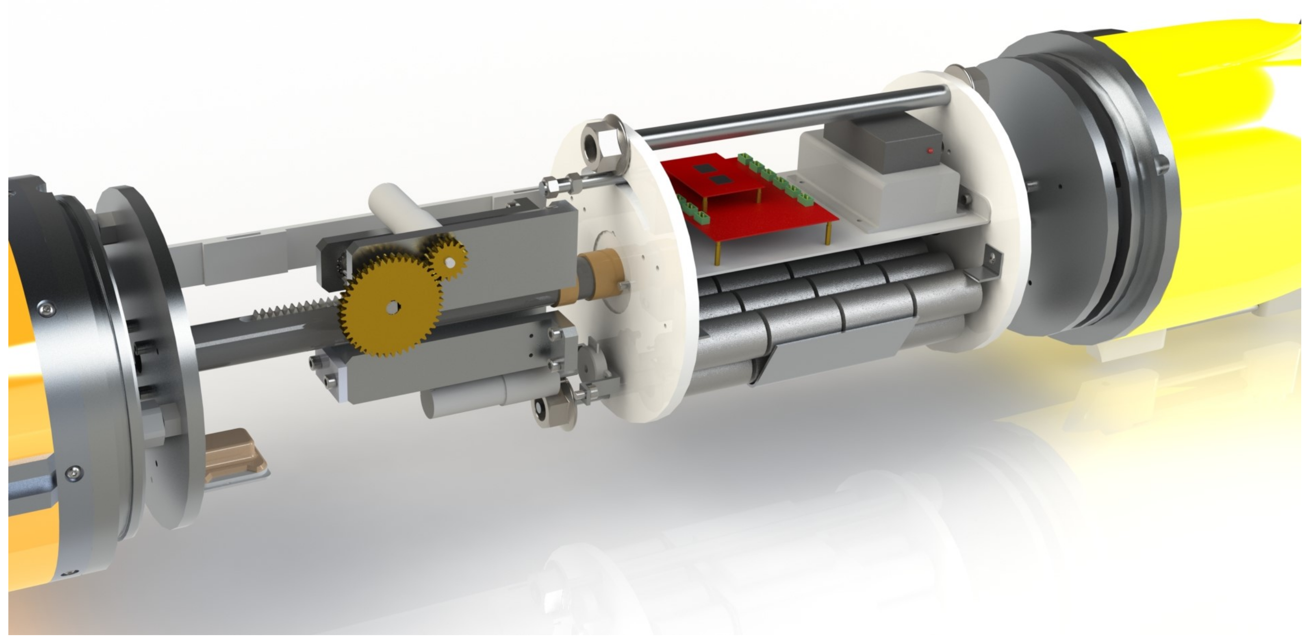
21]. In addition, due to the influence of hydrodynamics, the pitch of the glider will cause oscillation during the adjustment process, resulting in the decrease of control accuracy. So the displacement of the movable mass plays a key role in controlling the pitch of the glider. The position of the movable mass is driven by a drive system consisting of a DC motor and a gear train [22]. Therefore, the actuator constraints must be considered when designing the control inputs, because the actuator constraints limit the feasibility of the control inputs.
Another challenge for the precise pitch control of gliders is to achieve the suppression of disturbances by the control algorithm. Many outstanding researches have been carried out in the field of pitch control of underwater gliders [23,24,25]. Among them, the bang-bang control has the concise structure. It does not depend on the control model [26]. For these reason, bang-bang control acts the basic method for glider pitch control. However, the controlled quantity of bang-bang is difficult to coordinate between overshoot and high accuracy. Proportion integration differentiation (PID) is widely used in glider pitch control for its engineering feasibility [27]. However, PID does not perform convincingly in the face of pycnocline control. In our previous work, applying the ADRC to control the glider pitch angle was introduced [22]. However, the previous work does not sufficiently consider the actuator constraints. Based on the above discussion, we believe the anti-disturbance algorithm for glider traversing the pycnocline considering the specific hardware demanding investigation.
In this work, we propose the actuator constrained active disturbance rejection method for controlling the pitch of the glider in the presence of the pycnocline. Main contributions are concluded as follows. Firstly, we derive the dynamics model of the glider. On this basis, we analyze the longitudinal plane nonlinear motion model containing the variable buoyancy term. Secondly, we propose the ADRC control algorithm considering actuator constraints to alleviate the interference of the pycnocline and meet the practical situation of glider hardware. Finally, we propose the metrics for controlling pitch angle in the presence of the pycnocline. The simulation results show that the proposed method has significant improvement in control accuracy of pitch angle compared with the comparison methods.
The paper is organized as follows: Section 2 derives the glider dynamic model. Section 3 demonstrates the ACADRC. Section 4 introduces three typical structures of the pycnocline and the control metrics. Section 5 presents the numerical simulation results and discussions. Finally, conclusions are summarized.

2. Dynamic Model Derivation

The derivation of the glider dynamics model has been presented in many outstanding works, such as [17,28]. This section introduces our up to date work compared to [3]. We simplified the form of the glider mass matrix, thus facilitating the decoupling process of the matrix model. Moreover, the model is modified in terms of the correction of the buoyancy term and the accurate calculation of the added mass to better describe the effect of the buoyancy change caused by the pycnocline.

2.1. Model Derivations

The main parts of our developed underwater glider OUC-III are shown in Figure 1. To facilitate illustration, the inertial coordinate system, the body coordinate system, and the velocity coordinate system are introduced. Applying the Newton’s law in the inertial system, the general form of the forces exerted on the underwater glider is obtained, which is shown in Equation (1). The hydrodynamic forces and moments of the glider are described in the current coordinate system, while the hydrodynamic forces and moments can be represented in the body system by the transformation matrix between the current coordinate system and the machine system. The gravitational forces and moments represented in the inertial system can also be converted to the body system to represent the external forces exerted on the glider in the same coordinate system. Then, through transforming the expressions into the inertial system, the force analysis of the glider is completed, as demonstrated in Equation (2). Among them, the r v can be calculated through r v = m v 1 · ( m b r b + m m r m + m h r h ) .
p ˙ = i = 1 I f exti π ˙ = j = 1 I τ exti
R BI i = 1 I f exti = m o g R BI k + R BC [ D , SF , L ] T = [ F 1 , F 2 , F 3 ] T R BI j = 1 I τ exti = m v g r v × R BI k + R BC [ M 1 , M 2 , M 3 ] T = [ T 1 , T 2 , T 3 ] T
F 1 = m 0 g sin ( θ ) + L sin ( α ) D cos ( α ) F 2 = SF F 3 = m 0 g cos ( θ ) D sin ( α ) L cos ( α ) T 1 = M 1 cos ( α ) M 3 sin ( α ) T 2 = M 2 m b g r b 1 cos ( θ ) m h g r h 1 cos ( θ ) m m g r m 1 cos ( θ ) m h g r h 3 sin ( θ ) m m g r m 3 sin ( θ ) T 3 = M 1 sin ( α ) + M 3 cos ( α )
The calculation of components of the forces and moments in the body frame are depicted in Equation (3), where the transformation matrix R B I T and R B C are described by Equations (4) and (5).
R B I T = cos θ cos ψ sin ϕ sin θ cos ψ cos ϕ sin ψ cos ϕ sin θ cos ψ + sin ϕ sin ψ cos θ sin ψ cos ϕ cos ψ + sin ϕ sin θ sin ψ sin ϕ cos ψ + cos ϕ sin θ sin ψ sin θ sin ϕ cos θ cos ϕ cos θ
R B C = cos α · cos β cos α · sin β sin α sin β cos β 0 sin α · cos β sin α · sin β cos α
According to the Lagrangian modeling theory, we discuss the kinetic energy of the glider. The toral kinetic energy consists of the portion of the glider and the portion of the added mass (Equation (6)). The derivation of the total kinetic energy with respect to the generalized quantities q g yields the linear momentum and the angular momentum expressed in the body system (Equation (7)). Denote the generalized mass matrix as I M , then the derivatives of P and Π with respect to time can be obtained as shown in Equation (8). Equation (11) shows the six degrees of freedom of accelerations of the glider obtained by transforming Equation (8). The derivatives of linear momentum and angular momentum with respect to time is expressed with the help of the transformation relationship of the linear momentum and the angular momentum between the body coordinate system and the inertial system, see Equations (10) and (11). Moreover, the specific expression of the I ˙ M is shown in Equation (12).
T = T v + T f = 1 2 V Ω m v I m v r ^ v m v r ^ v J v V Ω + 1 2 V Ω M f C f T C f J f V Ω = 1 2 V Ω m v I + M f m v r ^ v + C f T m v r ^ v + C f J v + J f v Ω = 1 2 V Ω M C C T J V Ω
P Π = T q g = M C C T J q g = I M q g
Q = d p / d t d Π / d t = I ˙ M q g + q g ˙ I M
V ˙ Ω ˙ = I M 1 P ˙ Π ˙ I ˙ M V Ω
p = R BI T P π = R BI T Π + b × p
P ˙ = MV × Ω + R IB T i = 1 I f exti Π ˙ = C T V × Ω + C Ω × V + R IB T j = 1 I τ exti
I ˙ M = m ˙ b 0 0 0 m ˙ b r v 3 0 0 m ˙ b 0 m ˙ b r v 3 0 m v r ˙ v 1 + m ˙ b r v 1 0 0 m ˙ b 0 m v r ˙ v 1 m ˙ b r v 1 0 0 m ˙ b r v 3 0 0 0 m m r ˙ m 1 r m 3 m ˙ b r v 3 0 m v r ˙ v 1 m ˙ b r v 1 0 2 m m r ˙ m 1 r m 1 0 0 m v r ˙ v 1 + m ˙ b r v 1 0 m m r ˙ m 1 r m 3 0 2 m m r ˙ m 1 r m 1
b ˙ = R I B V , θ ˙ = 1 sin ϕ · tan θ cos ϕ · tan θ 0 cos ϕ sin ϕ 0 sin ϕ · sec θ cos ϕ · sec θ Ω
tan α = V 3 V 1 , sin β = V 2 V 1 2 + V 2 2 + V 3 2
Up to this point, all parameters in Equation (9) can be calculated. Combined with the specific kinematic equations (Equation (13)) and the expressions of hydrodynamic angles (Equation (14)), the simulation of the glider motion can be realized using the Runge-kutta method.

2.2. Longitudinal Model Considering Varying Seawater Density

This section introduces the longitudinal plane model of the glider. Since the movable mass of the glider keeps neutral and non-rotate, we denote the r v has the form as r v = [ r v 1 , 0 , r v 3 ] T . Moreover, for the vertical motion, V 2 , p and r maintains zero. Thus, the cross term of the added mass and the inertial hydrodynamic term driven by these motions is zero.
M = m 1 0 0 0 m 2 0 0 0 m 3 , J = j 1 0 j 4 0 j 2 0 j 4 0 j 3 , C = 0 c 1 0 c 2 0 c 3 0 c 4 0
I M 1 = i 11 0 i 13 0 i 15 0 0 i 22 0 i 24 0 i 26 i 31 0 i 33 0 i 35 0 0 i 42 0 i 44 0 i 46 i 51 0 i 53 0 i 55 0 0 i 62 0 i 64 0 i 66
i 11 = c 4 2 j 2 m 3 c 1 2 m 3 + c 4 2 m 1 j 2 m 1 m 3 , i 13 = c 1 c 4 c 1 2 m 3 + c 4 2 m 1 j 2 m 1 m 3 , i 15 = c 1 m 3 c 1 2 m 3 + c 4 2 m 1 j 2 m 1 m 3 , i 22 = j 1 j 3 + j 4 2 c 2 2 j 3 2 c 2 c 3 j 4 + c 3 2 j 1 j 1 j 3 m 2 + j 4 2 m 2 , i 24 = c 2 j 3 c 3 j 4 c 2 2 j 3 2 c 2 c 3 j 4 + c 3 2 j 1 j 1 j 3 m 2 + j 4 2 m 2 , i 26 = c 2 j 4 + c 3 j 1 c 2 2 j 3 2 c 2 c 3 j 4 + c 3 2 j 1 j 1 j 3 m 2 + j 4 2 m 2 , i 31 = c 1 c 4 c 1 2 m 3 + c 4 2 m 1 j 2 m 1 m 3 , i 33 = c 1 2 j 2 m 1 c 1 2 m 3 + c 4 2 m 1 j 2 m 1 m 3 , i 35 = c 4 m 1 c 1 2 m 3 + c 4 2 m 1 j 2 m 1 m 3 , i 42 = c 2 j 3 c 3 j 4 c 2 2 j 3 2 c 2 c 3 j 4 + c 3 2 j 1 j 1 j 3 m 2 + j 4 2 m 2 , i 44 = c 3 2 j 3 m 2 c 2 2 j 3 2 c 2 c 3 j 4 + c 3 2 j 1 j 1 j 3 m 2 + j 4 2 m 2 , i 46 = c 2 c 3 + j 4 m 2 c 2 2 j 3 2 c 2 c 3 j 4 + c 3 2 j 1 j 1 j 3 m 2 + j 4 2 m 2 , i 51 = c 1 m 3 c 1 2 m 3 + c 4 2 m 1 j 2 m 1 m 3 , i 53 = c 4 m 1 c 1 2 m 3 + c 4 2 m 1 j 2 m 1 m 3 , i 55 = m 1 m 3 c 1 2 m 3 + c 4 2 m 1 j 2 m 1 m 3 , i 62 = c 2 j 4 + c 3 j 1 c 2 2 j 3 2 c 2 c 3 j 4 + c 3 2 j 1 j 1 j 3 m 2 + j 4 2 m 2 , i 64 = c 2 c 3 + j 4 m 2 c 2 2 j 3 2 c 2 c 3 j 4 + c 3 2 j 1 j 1 j 3 m 2 + j 4 2 m 2 , i 66 = c 2 2 j 1 m 2 c 2 2 j 3 2 c 2 c 3 j 4 + c 3 2 j 1 j 1 j 3 m 2 + j 4 2 m 2 ,
The adjusted added mass cross term C f , leaves only the (2nd, 3rd) element c f 23 that is not zero. On this basis, we denote the M, J, C has the form as Equations (15) and (16) shows, where m 1 = m v + m f 1 , m 2 = m v + m f 2 , m 3 = m v + m f 3 , j 1 = j v 1 + j f 1 , j 2 = j v 2 + j f 2 , j 3 = j v 3 + j f 3 , j 4 = j v 4 and c 1 = m v r v 3 , c 2 = m v r v 3 + c f 1 , c 3 = m v r v 1 + c f 3 , c 4 = m v r v 1 + c f 2 . The I M 1 can be further expressed in Equation (16), where the elements are demonstrated in Equation (17). Taking the above results into Equation (9) and considering the characteristics of the glider’s vertical motion, the 3D of glider dynamic Equation is obtained.
V ˙ 1 V ˙ 3 q ˙ = i 11 i 13 i 15 i 31 i 33 i 35 i 51 i 53 i 55 · D cos ( α ) + L sin ( α ) m 0 g sin ( θ ) m 3 q V 3 + m ˙ b q r v 3 + m ˙ b V 1 D sin ( α ) L cos ( α ) + m 0 g cos ( θ ) + m 1 q V 1 + m ˙ b V 3 + q ( m ˙ b r v 1 r ˙ v 1 m v ) M 2 c 1 q V 3 + c 4 q V 1 + V 3 ( m ˙ b r v 1 r ˙ v 1 m v ) + m ˙ b r v 3 V 1 + 2 r ˙ m 1 m m q r m 1 + k
k = m b g r b 1 cos ( θ ) m h g r h 1 cos ( θ ) m m g r m 1 cos ( θ ) m h g r h 3 sin ( θ ) m m g r m 3 sin ( θ )
Then, the model for the vertical motion of the glider is described in Equation (20). This work considers the effect of pycnocline on glider pitch control. Thus, the density distribution of the seawater cannot be considered as uniform. We corrected m b to reflect the abrupt change of density, refer to Equation (21). In Equation (21), the ρ u represents the uniformly distributed density, while ρ v depicts the varying density. Furthermore, based on the partial derivative of density with respect to depth, we modified m ˙ b as Equation (22) shows, where d e p denotes the depth. m ˙ b and m b represent the buoyancy term in the uniformly distributed density field.
s ˙ 1 = V 1 cos θ V 3 sin θ s ˙ 3 = V 1 sin θ + V 3 cos θ θ ˙ = q V ˙ 1 = 1 c 1 2 m 3 + c 4 2 m 1 j 2 m 1 m 3 · { c 1 c 4 [ D sin ( α ) L cos ( α ) + m ˙ b V 3 + m 0 g cos ( θ ) + m 1 q V 1 + q ( m ˙ b r v 1 r ˙ v 1 m v ) ] + c 1 m 3 [ M 2 c 1 q V 3 + c 4 q V 1 + m ˙ b r v 3 V 1 + 2 r ˙ m 1 m m q r m 1 + k + V 3 ( m ˙ b r v 1 r ˙ v 1 m v ) ] + ( c 4 2 j 2 m 3 ) [ D cos ( α ) + L sin ( α ) + m ˙ b q r v 3 + m ˙ b V 1 m 0 g sin ( θ ) m 3 q V 3 ] } V ˙ 3 = 1 c 1 2 m 3 + c 4 2 m 1 j 2 m 1 m 3 · { c 1 c 4 [ D cos ( α ) + L sin ( α ) + m ˙ b q r v 3 + m ˙ b V 1 m 0 g sin ( θ ) m 3 q V 3 ] + c 4 m 1 [ M 2 c 1 q V 3 + c 4 q V 1 + m ˙ b r v 3 V 1 + 2 r ˙ m 1 m m q r m 1 + k + V 3 ( m ˙ b r v 1 r ˙ v 1 m v ) ] + ( c 1 2 j 2 m 1 ) [ D sin ( α ) L cos ( α ) + m ˙ b V 3 + m 0 g cos ( θ ) + m 1 q V 1 + q ( m ˙ b r v 1 r ˙ v 1 m v ) ] } q ˙ = 1 c 1 2 m 3 + c 4 2 m 1 j 2 m 1 m 3 · { c 1 m 3 [ D cos ( α ) + L sin ( α ) + m ˙ b q r v 3 + m ˙ b V 1 m 0 g sin ( θ ) m 3 q V 3 ] + c 4 m 1 [ D sin ( α ) L cos ( α ) + m ˙ b V 3 + m 0 g cos ( θ ) + m 1 q V 1 + q ( m ˙ b r v 1 r ˙ v 1 m v ) ] m 1 m 3 [ M 2 c 1 q V 3 + c 4 q V 1 + m ˙ b r v 3 V 1 + 2 r ˙ m 1 m m q r m 1 + k + V 3 ( m ˙ b r v 1 r ˙ v 1 m v ) ] } u i n = r m 1
m b = m b ρ v ρ u
m ˙ b = m ˙ b ρ v d e p ρ u d e p

2.3. Parameters Determination

In our previous work [3], we presented the determination of hydrodynamic parameters for the OUC-III glider, and the results are listed in Table 1. According to the research in [17], parameters in Table 1 is determined by the mechanical shell. Once these parameters are calculated via the curve fitting techniques, the hydrodynamic forces and momentum are able to determine combined with the specific hydrodynamic angles and the velocities. However, the added mass appeared in Equation (20) changes with the density. Other physical parameters of the OUC-III glider are listed in Table 2.
In this work, we calculated the added mass of OUC-III using the hess-smith panel method [29]. Firstly, the glider surface is divided in a continuous triangular panels using finite element software. Then, the node information is resolved from the result of the division, and the area, center and normal of the surface elements are calculated based on the obtained nodes, as shown in Figure 2. Then, construct the linear system of equations about the intensity of the Rankine source σ , as Equation (23). Where V f is the value of the velocity at infinity, n represent the direction of calculation, the number of the system of equations is the number of elements. The resulting σ is brought into Equation (24) to calculate the velocity potential Φ . The additional mass can be calculated from Equation (25). Note that the added mass is related to the density of the fluid. So the motion of the glider in the pycnocline needs to consider the change of the added mass.
2 π σ ( p a ) + j = 1 N σ j Δ Q j n p a 1 r p a q a d s q a = V f · n
Φ ( p a ) = Δ s σ ( q a ) r p a q a d s
λ i j = ρ i = 1 N Φ i n j d s
Equation (26) shows the added mass terms for ρ = 1000 kg / m 3 , and these matrices need to be corrected for fluid density during the glider profile.
M f = 1.94 0 0 0 65.51 0 0 0 79.46 , J f = 2.04 0 0 0 27.98 0 0 0 28.30 , C f = 0 0.19 0 0 0 4.46 0 2.94 0

3. The Actuator Constrained Active Disturbance Rejection Control

This section introduces the concept of the actuator constraints and the basic structure of ACADRC. This part also introduces the basic settings of the control methods involved in the comparison in Section 5.

3.1. The Actuator Constrains

As discussed before, the buoyancy engine is prone to interfered by the environment. Furthermore, the OUC-III glider is not equipped with the elevator, which makes the effective maneuverability of hydrodynamics not accessible. So, the key parameter for pitch control is the longitudinal displacement of the movable mass. The physical system of the glider’s movable mass is shown in Figure 3.
The planetary gear is driven by a DC motor fixed to the movable mass block. The axial displacement of the movable mass is adjusted by meshing with the screw rod. Assuming that the movable mass of the glider has a displacement r m 1 along the axial direction, resulting in the overall center of gravity of the glider moving the distance of l = m m r m 1 / m v . Considering that the metacentric height of the glider is h, then the steady value of the glider pitch angle manipulated by the movable mass can be expressed by Equation (27). In order to ensure the driving effect of the movable mass at the ultimate angle, the axial tension of the screw corresponding to the extreme pitch angle should be calculated. The calculation is shown in Equation (28), where the θ s m represent the extreme pitch angle. Accordingly, the desired torch of the screw under such case can be calculated referring to the lead angle of screw and the equivalent coefficient of friction as Equation (29) illustrated.
θ s = arctan ( m m r m 1 m v h )
F r = m m g cos θ s m
T r = F r d r 2 2 tan ( μ + ϵ )
Denote the reduction gear ratio of planetary gear as i, the maximum continuous output torque as T c , and the transmission efficiency as η . Then the continuous output torque of DC motor can be calculated as Equation (30). The type of DC motor is selected according to the T m , and the actuator constraint for glider pitch control can be calculated referring to the rated speed of the DC motor. The calculated v L is 1.3 × 10 3 m/s, which means that the control algorithm of the pitch must follow the constraints of the calculated v L . The control algorithm cannot exert influence on the pitch angle according to the ideal control input, which affects the control effect, but is close to the actual physical system. Moreover, the movement of the movable mass relies on a linear potentiometer to decode the control signal. This also contributes to the actuator constraints.
T m = T c i η
v L = n 60 × i L

3.2. The ACADRC

The active disturbance rejection control mainly consists of the tracking differentiator (TD), the nonlinear state error feedback (NLSEF) and the extended state observer (ESO) as shown in Figure 4. The TD section arranges the transition process for the reference input signal, and this design avoids the drastic tracking of the abruptly changing reference signal. At the same time TD generates the differential signal of the reference output. The formulas of the TD are show in Equation (32), where r 0 denotes the speed factor, h is the filter factor, and fhan represents the optimal control function. The ESO estimates the system output and the total disturbance in real time, and generates the system error by making a difference with the differential signal generated by the TD. By using the system output signal θ and the input signal u to track and estimate the system state and disturbances, it is the key to achieve the suppression of environmental disturbances. Its principle is listed in Equation (33). β 01 , β 01 and β 01 are the adjustable parameters and z 1 , z 2 , z 3 are the estimations of the pitch angle and its derivatives of each order, respectively. fal is a continuous power series function with linear segments near the origin [22].
e = θ r 1 θ f h = fhan ( e , θ r 2 , r 0 , h ) θ r 1 = θ r 1 + h θ r 2 θ r 2 = θ r 2 + h f h
e = z 1 θ d z 1 = z 2 β 01 fal ( e , a 1 , δ ) d z 2 = z 3 β 02 fal ( e , a 2 , δ ) + b 0 u d z 3 = β 03 fal l ( e , a 3 , δ )
NLSEF can be expressed as Equation (34). The control output of the classical ADRC can be derived via the output u 0 combined with the estimation of the disturbance z 3 . However, this control output does not fully consider the actuator constraints. By mapping the output u to the action space of the movable mass of the glider and combining it with the properties of the potentiometer-based control of the actuator, the output of ACADRC can be obtained.
e 1 = θ r 1 z 1 e 2 = θ r 2 z 2 u 0 = β 1 fal ( e 1 , a 4 , δ u ) + β 2 fal ( e 2 , a 2 , δ u )

3.3. The Comparison Methods

In this work, to illustrate the control effect of the proposed ACADRC, we chose bang-bang control and PID control as the comparison methods. They are both commonly used methods in underwater glider engineering applications.The idea of bang-bang control is to output the actuator adjustment signal by comparing the the current controlled state with the target. In OUC-III, the movable mass has the coordinates [ 0.65 , 0 , 0 ] T meters in the body-frame. Furthermore, the adjustable range is 0.65 ± 0.07 . In order to prevent the actuator from excessive oscillation under bang-bang control, we selected the range of ± 1 degree from the target pitch as the termination band of control. The PID constructs the actuator target signal based on the error between the current pitch angle and the target pitch angle. The incremental PID control is selected in this work, and the principle is shown in Equation (35), where Δ θ ( k ) = θ ( k ) θ ( k 1 ) . The selected parameters are k p = 0.0005 , k i = 0.0000015 , k d = 0.0000008 .
Δ u = k p [ Δ θ ( k ) Δ θ ( k 1 ) ] + k i Δ θ ( k ) + k d [ Δ θ ( k ) 2 Δ θ ( k 1 ) + Δ θ ( k 2 ) ]

4. Discussion on Pycnocline and Control Metrics

This section introduces the structure of the pycnocline used in Section 5. We also introduce the metrics that depict the effect of pitch control in the presence of the pycnocline.

4.1. Three Typical Types of Pycnocline

Three typical structures of pycnocline are adopted in this work, which are the typically-discussed pycnocline with three stratified layer [30], the inverted pycnocline [31] and the dual-pycnocline (double pycnocline) [32]. To facilitate referring, denote them as pycnocline 1, pycnocline 2, pycnocline 3. Their density-depth curves are shown in Figure 5.
The red dot in the figure depicts the boundaries of pycnocline. In the typically-discussed pycnocline, the partial derivatives of the density with respect to depth are smaller in both the upper and lower layers of the jump layer, which causes the density of seawater in these two layers to increase slowly with depth. However, in the jump layer, the density increases steeply within a limited depth, which leads to undesired changes in pitch angle control. Generally, the density of seawater increases with depth, but in the inverted pycnocline, the density of seawater underwater is less than that near the surface. This may lead to a steep drop in depth for the underwater vehicle and also cause interference to the pitch angle. The dual-pycnocline can be originally considered as a continuous typically-discussed pycnocline, whose density exerts disturbances on the glider in two depth intervals. It causes multiple oscillations of the pitch angle control. The specific parameters of the three pycnoclines used in this section are listed in Table 3, where the u b represents the upper boundaries, and l b illustrates the lower boundaries. The i n t e n s i t y demonstrates the partial of density with respect to the depth among the jump layer, while the u i and l i depicts the intensity of the upper and lower layer of the pycnocline, respectively. Taking the pycnocline 1 as an example, we demonstrate the interference of the pycnoncline exerted on to the glider pitch. As Figure 6 shows, the green band illustrates the pycnocline. It can be observed that the pycnocline influences the pitch of the UGs significantly.

4.2. The Control Metrics of Pitch Control

As shown in Figure 7, the profile of the glider can be divided into four processes. They are the accelerating diving phase, the stable diving phase, the dive-surfacing switching phase and the stable surfacing phase. Among them, the accelerating diving stage is more aggressive in pitch angle control in order to reach the target pitch angle as soon as possible. After reaching flare point (1), the glider is controlled according to the diving target angle. At (3), the glider dives to the set depth and starts to adjust buoyancy and attitude to prepare for surfacing. After the adjustment of the switching process, the glider reaches the flare point (2), which means that the glider starts to control the floating pitch angle. The determination of the flare time is defined in Equation (36). The δ depicts the error to index. We also define the t m to illustrate the time when the glider reach the set depth, which can be found in Equation (37). To determine flare point (2) (denotes as t f 1 ), the 19.1 and the + δ are chosen. Together with the t m , the interval for continuous controlling the pitch angle during the dive phase can be selected. As shown in Equation (38). The mean and variance of the glider pitch angle in this selected interval can reflect the control effect of the specific control algorithm.
t f = sort { abs [ θ ± 19.1 δ ] } [ 1 ]
t m = index argmin { abs [ ( s 3 s s e t ) ] }
t e r v a l = t m t f 1
m e a n = t = i i = t f 1 , , t m θ i length ( θ )
v a r = t = i i = t f 1 , , t m ( θ i m e a n ) 2 length ( θ )

5. Numerical Simulation Results and Discussion

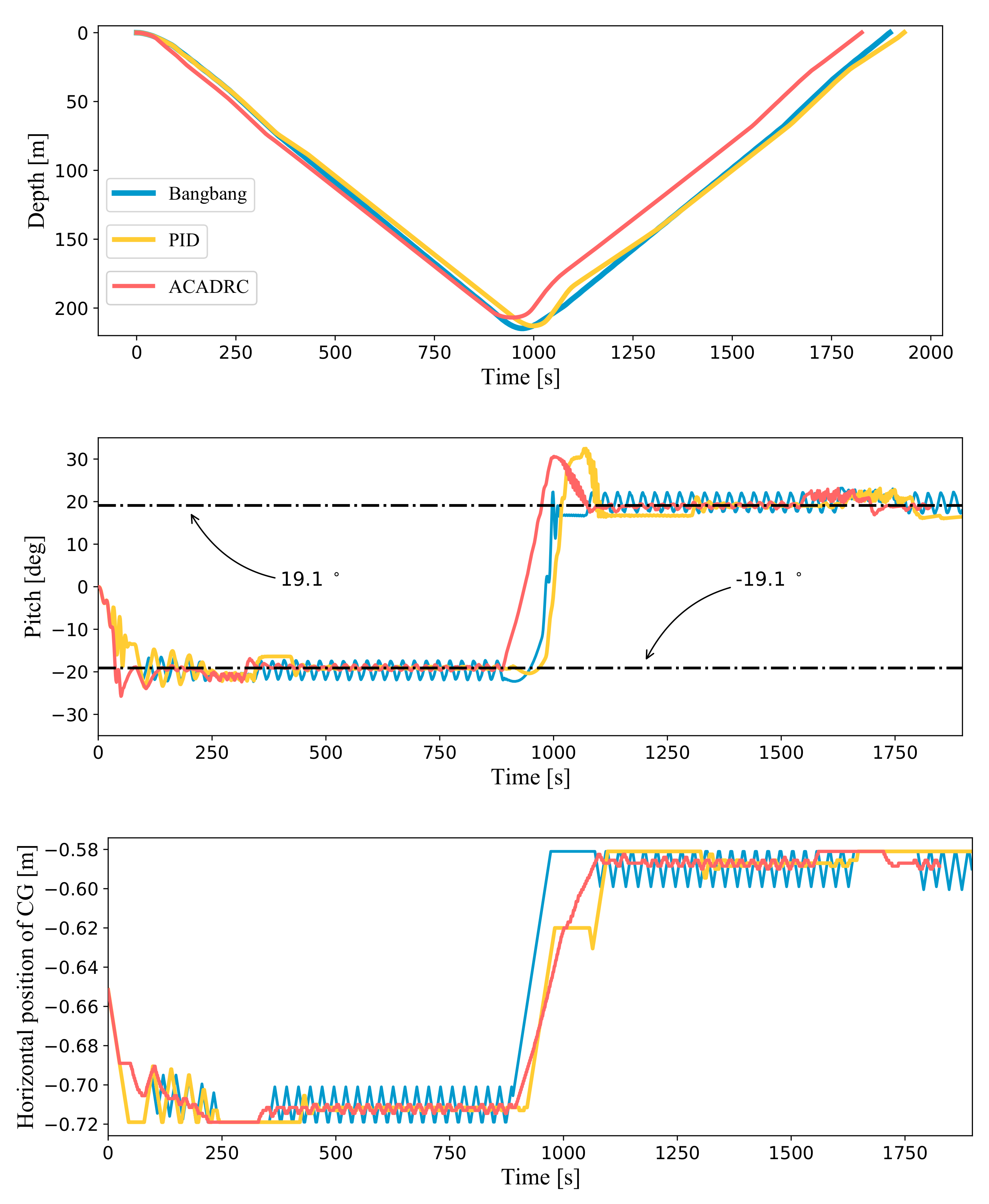
To examine the ACADRC control effect, we conduct the motion simulation of the glider in the presence of three types of pycnocline. The bang-bang control and the PID control are introduced to compare the control effect. The diving depth of the glider is set to 200 m. Because the interference of the pycnocline on the pitch control is mainly focused, we consider the movable mass of the glider as non-rotatable. Therefore, the roll angle and the heading angle of the glider are all zero degree during the simulation. Figure 8, Figure 9 and Figure 10 present the motion simulation results, which consists of the depth results and the pitch results.
According to the simulation results. Although bang-bang control is a common control techniques for engineering applications. However, it leads to drastic oscillations in pitch angle and insufficient suppression in the face of disturbances caused by density jumps. However, the pitch angle under bang-bang control did not show significant overshoot. PID control has a significant improvement in accuracy compared to bang-bang control. However, the control effect performs unstably between the diving and floating. Furthermore, the control results show that the pitch angle has interval steady-state errors and is seriously affected by density disturbances. In addition, the pitch angle of PID control has significant overshoot.
The pitch angle controlled by ACADRC is more stable than the comparison method. The pitch angle can be controlled around the target pitch angle. Furthermore, it has a better suppression effect on density interference than the comparison method. The disadvantage lies in that the ACADRC still has overshoot. However, the overshoot of both ACADRC and PID occurs in the surfacing phase and the glider does not reach the flare point. As defined in Section 4.2, the control metrics for the pitch control during the selected interval are listed in Table 4. The results indicate that the ACADRC has the comprehensive performance over the comparison methods in the aspect of lower variance and closer mean value to the target pitch.
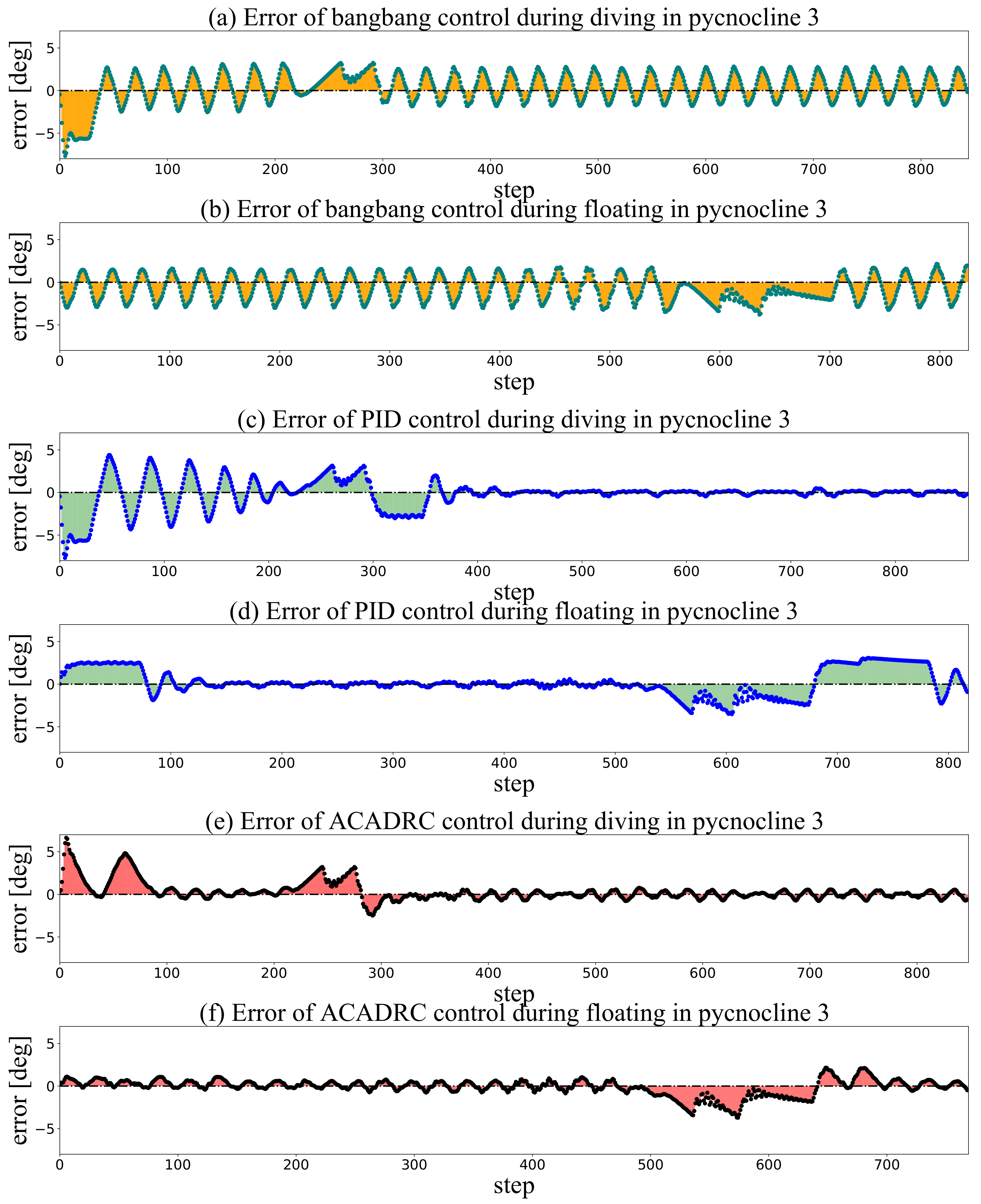
To better visualize the error of the controlled pitch with respect to the target pitch, we provide the Figure 11, Figure 12 and Figure 13. For each control algorithm, we show error plots for the diving control phase and the floating control phase. According to the figures, the pitch angle under bang-bang control fluctuates up and down along the target pitch, resulting in poorer accuracy. In contrast, PID has high control accuracy in some stages, and even performs best in all three algorithms. However, the PID cannot achieve the globally accurate pitch control. The performance of ACADRC is weaker than PID in some areas, but the control effect is smoother in the whole control cycle and the suppression of density variation is better than the comparison method. It is worth noting that the glider cannot suppress the deviation of the pitch angle even if the movable mass is adjusted to the limit position due to the abrupt change of density in the pycnocline. At this point, all three discussed methods are unable to control the pitch angle to maintain the set angle. However, ACADRC can make a continuous estimation of the disturbance to compensate the control signal and make the pitch angle return to the set state quickly. In contrast, the PID control still suffers from oscillations and delays. Therefore, we believe that ACADRC is capable of accurately controlling the pitch in the presence of the pycnocline.

6. Conclusions

In this work, we have discussed the problem of accurate control of the pitch angle of the glider in the presence of the pycnocline. We have established the longitudinal model of the glider considering density variation based on the derived six-degree-of-freedom glider dynamics equations. On this basis, the influence of three typical pycnocline structures on the pitch of the glider has been considered. The simulation results have shown that the abrupt density change caused by pycnocline will bring significant disturbance to the pitch angle. The actuator constraints of the glider in conjunction with the hardware characteristics of the glider have been discussed. Under this constraint, the input of the control algorithm cannot be fully mapped to the actuator action, which has deteriorated the effectiveness of the control algorithm. The ACADRC has been proposed for this purpose, which, on the one hand, has allowed estimating disturbances in real time during the control process. At the same time, the output has been improved to better adapt to the actuator constraints for the purpose of achieving better pitch control results. The simulations have shown the advantages of the proposed method in terms of pitch control accuracy compared to bang-bang control and PID control.
Future work will focus on further suppression of pitch angle errors caused by pycnocline, as well as field tests.

Author Contributions

Conceptualization, W.Z. and M.C.; methodology and software, W.Z. and X.L.; validation, D.S. and T.G.; resources, D.S.; writing—original draft preparation, W.Z.; writing—review and editing, T.G., M.C. All authors have read and agreed to the published version of the manuscript.

Funding

This research was supported by the Fundamental Research Funds for the Central Universities (Grant No. 202061004).

Institutional Review Board Statement

Not applicable.

Informed Consent Statement

Not applicable.

Data Availability Statement

The experimental data supporting this study are provided within this paper.

Acknowledgments

We would like to thank the Underwater Robot Laboratory of Ocean University of China for its hardware and software support for this work.

Conflicts of Interest

The authors declare that they have no known competing financial interests or personal relationships that could have appeared to influence the work reported in this paper.

Nomenclature

m b mass of the bladder
m s mass of the glider static components
m m mass of the movable block
m v mass of the vehicle m v = m b + m s + m m
m 0 equivalent mass of net buoyancy
J v inertia of glider: J v = [ [ j v 1 , 0 , j v 4 ] , [ 0 , j v 2 , 0 ] , [ j v 4 , 0 , j v 3 ] ]
J s inertia of the glider’s static components
M f added mass matrix: M f = d i a g ( m f 1 , m f 2 , m f 3 )
J f added inertia matrix: J f = d i a g ( j f 1 , j f 2 , j f 3 )
C f added coupling matrix: [ [ 0 , c f 1 , 0 ] , [ 0 , 0 , c f 2 ] , [ 0 , c f 3 , 0 ] ]
r v position vector of the vehicle in the body coordinate system
r s position vector of static mass in the body coordinate system
r m position vector of the movable mass in the body coordinate system
r b position vector of the bladder in the body coordinate system
l v position vector of the vehicle in the inertia coordinate system
l h position vector of static mass in the inertia coordinate system
l m position vector of the movable mass in the inertia coordinate system
l b position vector of the bladder in the inertia coordinate system
V translational velocity in the body coordinate system, V = [ V 1 , V 2 , V 3 ] T
Ω angular velocity in the body coordinate system, Ω = [ p , q , r ] T
s glider position in the inertia coordinate system, s = [ s 1 , s 2 , s 3 ] T
b position vector of glider’s center of buoyancy in the inertia coordinate system
θ glider attitude in the inertia coordinate system θ = [ ϕ , θ , ψ ] T
P linear momentum of glider in the body coordinate system
p linear momentum of glider in the inertia coordinate system
Π angular momentum of glider in the body coordinate system
π angular momentum of the glider in the inertia coordinate system
f exti the ith external force expressed in the inertia coordinate system
τ exti the ith external moment expressed in the inertia coordinate system
F gra gravitational forces in the body coordinate system
T gra gravitational moments in the body coordinate system
α the angle of attack
β the side slip angle
T hyd hydrodynamic moments in the currents coordinate system
F hyd hydrodynamic forces in the currents coordinate system
L lift force in the currents coordinate system,    L = ( K L 0 + K L α ) V 2
D drag force in the currents coordinate system,    D = ( K D 0 + K D α 2 ) V 2
SF lateral force in the currents coordinate system, SF = K β β V 2
F i ( i = 1 , 2 , 3 ) moments around three axes in the currents coordinate system
M i ( i = 1 , 2 , 3 ) moments around three axes in the currents coordinate system
Qgeneralized force
q g generalized quantity
Tthe kinetic energy of the glider system
T f added kinetic energy in the body frame
T v kinetic energy of the vehicle
ttime
r m 1 translational position of m m in body frame
hthe metacentric height
θ s m the extreme of the pitch angle
dthe diameter of the screw rod
ϵ the lead angle of screw
η the transmission efficiency
v L the constrained velocity of the movable mass (the actuator constraints)
μ the equivalent coefficient of friction
ithe reduction gear ratio of planetary gear
Lthe length of the screw rot
nthe rated speed of the DC motor

References

  1. Petritoli, E.; Leccese, F.; Cagnetti, M. High accuracy buoyancy for underwater gliders: The uncertainty in the depth control. Sensors 2019, 19, 1831. [Google Scholar] [CrossRef] [PubMed] [Green Version]
  2. Wu, H.; Niu, W.; Wang, S.; Yan, S. An optimization method for control parameters of underwater gliders considering energy consumption and motion accuracy. Appl. Math. Model. 2021, 90, 1099–1119. [Google Scholar] [CrossRef]
  3. Sun, W.; Zang, W.; Liu, C.; Guo, T.; Nie, Y.; Song, D. Motion pattern optimization and energy analysis for underwater glider based on the multi-objective artificial bee colony method. J. Mar. Eng. 2021, 9, 327. [Google Scholar] [CrossRef]
  4. Claus, B.; Bachmayer, R.; Cooney, L. Analysis and development of a buoyancy-pitch based depth control algorithm for a hybrid underwater glider. In Proceedings of the 2012 IEEE/OES Autonomous Underwater Vehicles (AUV), Southampton, UK, 24–27 September 2012; pp. 1–6. [Google Scholar]
  5. Tatone, F.; Vaccarini, M.; Longhi, S. Modeling and attitude control of an autonomous underwater glider. IFAC Proc. Vol. 2009, 42, 217–222. [Google Scholar] [CrossRef]
  6. De Fommervault, O.; Besson, F.; Beguery, L.; Page, Y.L.; Lattes, P. Seaexplorer underwater glider: A new tool to measure depth-resolved water currents profiles. In Proceedings of the OCEANS 2019-Marseille, Marseille, France, 17–20 June 2019; pp. 1–6. [Google Scholar]
  7. Ma, W.; Wang, Y.; Wang, S.; Zhang, H.; Zhang, H.; Gong, Q. Absolute current estimation and sea-trial application of glider-mounted ad2cp. J. Coast. Res. 2019, 35, 1343–1350. [Google Scholar] [CrossRef]
  8. Yang, Y.; Liu, Y.; Wang, S.; Zhang, L.; Wang, Y.; Zhang, H. Evaluation models and criteria of motion performance for underwater gliders. Appl. Ocean. Res. 2019, 102, 102286. [Google Scholar] [CrossRef]
  9. Song, D.; Chen, Z.; Fu, J.; Wang, X.; Jiang, W.; Wu, J. Novel underwater glider-based absolute oceanic current observation solutions. IEEE Sens. J. 2020, 21, 8045–8054. [Google Scholar] [CrossRef]
  10. Rusello, P.J.; Yahnker, C.; Morris, M. Improving depth averaged velocity measurements from seaglider with an advanced acoustic current profiler, the nortek ad2cp-glider. In Proceedings of the 2012 Oceans, Hampton Roads, VA, USA, 14–19 October 2012; pp. 1–8. [Google Scholar]
  11. Cassar, C. An Introduction to Underwater Gliders. Available online: http://ioi.research.um.edu.mt/GliderSouth/index.php/welcome/gliders_info (accessed on 15 September 2021).
  12. Zhang, Y.; Wu, D.-X.; Lin, X.-P. A study of thermocline and pycnocline calculations in the east china sea in summer. J. Ocean. China 2006, 36, 1–7. [Google Scholar]
  13. Ayyemperumal, S.; Jeyaseelan, T.; Minamino, T.; Arima, M. Development of an underwater glider with density-difference-engine. In Proceedings of the 2018 World Automation Congress (WAC), Stevenson, WA, USA, 3–6 June 2018; pp. 1–5. [Google Scholar]
  14. Zhou, H.; Fu, J.; Liu, C.; Zeng, Z.; Yu, C.; Yao, B.; Lian, L. Dynamic modeling and endurance enhancement analysis of deep-sea gliders with a hybrid buoyancy regulating system. Ocean. Eng. 2020, 217, 108146. [Google Scholar] [CrossRef]
  15. Liu, Y.; Ma, J.; Ma, N.; Zhang, G. Path planning for underwater glider under control constraint. Adv. Mech. Eng. 2017, 9, 1687814017717187. [Google Scholar] [CrossRef]
  16. Kahveci, N.E.; Ioannou, P.A.; Mirmirani, M.D. A robust adaptive control design for gliders subject to actuator saturation nonlinearities. In Proceedings of the 2007 American Control Conference, New York, NY, USA, 9–13 July 2007; pp. 492–497. [Google Scholar]
  17. Zhang, S.; Yu, J.; Zhang, A.; Zhang, F. Spiraling motion of underwater gliders: Modeling, analysis, and experimental results. Ocean Eng. 2013, 60, 1–13. [Google Scholar] [CrossRef]
  18. Petritoli, E.; Leccese, F.; Cagnetti, M. A high accuracy buoyancy system control for an underwater glider. In Proceedings of the 2018 IEEE International Workshop on Metrology for the Sea; Learning to Measure Sea Health Parameters (MetroSea), Bari, Italy, 8–10 October 2018; pp. 257–261. [Google Scholar]
  19. Petritoli, E.; Leccese, F. A high accuracy navigation system for a tailless underwater glider. In Proceedings of the IMEKO TC19 Workshop on Metrology for the Sea, MetroSea, Naples, Italy, 11–13 October 2017. [Google Scholar]
  20. Petritoli, E.; Leccese, F.; Cagnetti, M. Underwater Gliders: Mission Profiles and Utilisation Strategies in the Mediterranean Sea. In Proceedings of the 2019 IMEKO TC19 International Workshop on Metrology for the Sea: Learning to Measure Sea Health Parameters, Genova, Italy, 3–5 October 2019; pp. 254–258. [Google Scholar]
  21. Wu, H.; Niu, W.; Wang, S.; Yan, S. Sensitivity analysis of control parameters errors and current parameters to motion accuracy of underwater glider using sobol’ method. Appl. Ocean. Res. 2021, 110, 102625. [Google Scholar] [CrossRef]
  22. Guo, T.; Song, D.; Li, K.; Li, C.; Yang, H. Pitch angle control with model compensation based on active disturbance rejection controller for underwater gliders. J. Coast. Res. 2020, 36, 424–433. [Google Scholar] [CrossRef]
  23. Tchilian, R.d.; Rafikova, E.; Gafurov, S.A.; Rafikov, M. Optimal control of an underwater glider vehicle. Procedia Eng. 2017, 176, 732–740. [Google Scholar] [CrossRef]
  24. Noh, M.M.; Arshad, M.R.; Mokhtar, R.M. Depth and Pitch Control of Usm Underwater Glider: Performance Comparison pid vs. lqr. Indian J.-Geo-Mar. Sci. 2011, 40, 200–206. [Google Scholar]
  25. Cao, J.; Cao, J.; Yao, B.; Lian, L. Dynamics and adaptive fuzzy turning control of an underwater glider. In Proceedings of the OCEANS 2015-Genova, Genova, Italy, 18–21 May 2015; pp. 1–7. [Google Scholar]
  26. Mitchell, B.; Wilkening, E.; Mahmoudian, N. Developing an underwater glider for educational purposes. In Proceedings of the 2013 IEEE International Conference on Robotics and Automation, Karlsruhe, Germany, 6–10 May 2013; pp. 3423–3428. [Google Scholar]
  27. Ullah, B.; Ovinis, M.; Baharom, M.B.; Javaid, M.; Izhar, S. Underwater gliders control strategies: A review. In Proceedings of the 2015 10th Asian Control Conference (ASCC), Kota Kinabalu, Malaysia, 31 May–3 June 2015; pp. 1–6. [Google Scholar]
  28. Singh, Y.; Bhattacharyya, S.K.; Idichandy, V.G. CFD approach to steady state analysis of an underwater glider. In Proceedings of the 2014 Oceans-St. John’s, St. John’s, NL, Canada, 14–19 September 2014; pp. 1–5. [Google Scholar]
  29. Sahin, I.; Crane, J.W.; Watson, K.P. Application of a panel method to hydrodynamics of underwater vehicles. Ocean Eng. 1997, 24, 501–512. [Google Scholar] [CrossRef]
  30. Cheng, M.-H.; Hsu, J.R.-C. Effects of varying pycnocline thickness on interfacial wave generation and propagation. Ocean Eng. 2014, 88, 34–45. [Google Scholar] [CrossRef]
  31. Church, T.M.; Mooers, C.N.; Voorhis, A.D. Exchange processes over a middle atlantic bight shelfbreak canyon. Estuar. Coast. Shelf Sci. 1984, 19, 393–411. [Google Scholar] [CrossRef]
  32. Shaw, J.; Stastna, M. Feature identification in time-indexed model output. PLoS ONE 2019, 14, e0225439. [Google Scholar] [CrossRef] [PubMed]
Figure 1. The OUC-III underwater glider systems. As indicated by the serial numbers, they illustrate ① the mechanical shell, ② the sampling loads, ③ horizontal wings, ④ the CTD profiler, ⑤ the vertical wing, ⑥ the antenna, ⑦ the electronic control unit, ⑧ the actuating system of the movable mass and ⑨ the buoyancy engine, respectively.
Jmse 09 01013 g001
Figure 2. The division of the glider surface. The area, center and normal of the surface element are also illustrated. Note that the normal is pointed inside the panel.
Jmse 09 01013 g002
Figure 3. The physical system of the glider’s movable mass.
Jmse 09 01013 g003
Figure 4. The structure of the ACADRC.
Jmse 09 01013 g004
Figure 5. The density distributions in three typical types of pycnocline.
Jmse 09 01013 g005
Figure 6. The density distributions in three typical types of pycnocline.
Jmse 09 01013 g006
Figure 7. The profile division of the glider.
Jmse 09 01013 g007
Figure 8. Glider motion simulation with the presence of pycnocline 1.
Jmse 09 01013 g008
Figure 9. Glider motion simulation with the presence of pycnocline 2.
Jmse 09 01013 g009
Figure 10. Glider motion simulation with the presence of pycnocline 3.
Jmse 09 01013 g010
Figure 11. The pitch control errors with respect to the reference angle ( 19 . 1 ° in the diving phase and 19 . 1 ° in the floating phase) with the presence of the typical pycnocline.
Jmse 09 01013 g011
Figure 12. The pitch control errors with respect to the reference angle ( 19 . 1 ° in the diving phase and 19 . 1 ° in the floating phase) with the presence of the inverted pycnocline.
Jmse 09 01013 g012
Figure 13. The pitch control errors with respect to the reference angle ( 19 . 1 ° in the diving phase and 19 . 1 ° in the floating phase) with the presence of the dual-pycnocline.
Jmse 09 01013 g013
Table 1. Hydrodynamic parameters of OUC-III.
ParametersValues
K D 0 8.669
K D 612.712
K β −67.415
K L 0 −2.223
K L 572.727
K M R −38.955
K P −23.694
K M 0 0.858
K M −53.524
K q −155.809
K M Y 77.862
K r −280.766
Table 2. Physical parameters of OUC-III.
ParametersValues
m m 76.600 kg
m h 9.400 kg
m b [ 1 , 1 ] kg
J s d i a g ( [ 0.154 , 28.365 , 28.243 ] )
r h [ 0.080 , 0 , 0.014 ] T
r b [ 0.897 , 0 , 0 ] T
Table 3. Physical parameters of OUC-III.
PropertiesPycnocline 1Pycnocline 2Pycnocline 3
u b 30 m50 m40 m, 80 m
l b 70 m70 m55 m, 100 m
i n t e n s i t y 0.15−0.130.15, 0.11
u i 0.02−0.0010.015, 0.01
l i 0.010.0060.01, 0.006
Table 4. Results of numerical simulations.
Pycnocline 1
MetricsBangbangPIDACADRC
t f 1 545444
t m 889920883
t e r v a l 1 835866839
m e a n 1 −19.526−18.912−19.319
v a r 1 3.6833.2551.437
t f 2 107811011071
t e 189719331826
t e r v a l 2 819832755
m e a n 2 20.01618.53419.336
v a r 2 2.5543.0761.210
Pycnocline 2
MetricsBangbangPIDACADRC
t f 1 919144
t m 946959927
t e r v a l 1 855868883
m e a n 1 −19.365−19.326−19.421
v a r 1 3.4010.9751.315
t f 2 109711161091
t e 198819811906
t e r v a l 2 891865815
m e a n 2 19.28018.97719.119
v a r 2 4.05612.4770.737
Pycnocline 3
MetricsBangbangPIDACADRC
t f 1 545444
t m 898924892
t e r v a l 1 844870848
m e a n 1 −19.415−18.932−19.226
v a r 1 3.6672.9341.303
t f 2 105611091071
t e 188219271840
t e r v a l 2 826818769
m e a n 2 19.91018.88919.217
v a r 2 2.2952.2070.915
Publisher’s Note: MDPI stays neutral with regard to jurisdictional claims in published maps and institutional affiliations.

