Article

Future Changes in Built Environment Risk to Coastal Flooding, Permanent Inundation and Coastal Erosion Hazards

1
National Institute of Water and Atmospheric Research, P.O. Box 11115, Hamilton 3251, New Zealand
2
Tonkin and Taylor Ltd., P.O. Box 317, Tauranga 3140, New Zealand
*
Author to whom correspondence should be addressed.
J. Mar. Sci. Eng. 2021, 9(9), 1011; https://doi.org/10.3390/jmse9091011
Submission received: 5 August 2021 / Revised: 31 August 2021 / Accepted: 7 September 2021 / Published: 15 September 2021
(This article belongs to the Section Marine Hazards)

Abstract

:
Sea-level rise will cause erosion of land, deeper and increasingly frequent flooding and will eventually permanently inundate low-elevation land, forcing the adaptation of seaside communities to avoid or reduce risk. To inform adaptation planning, we quantified the effects of incremental relative sea-level rise (RSLR) on exposed land area, number and replacement value of buildings within Tauranga Harbour, New Zealand. The assessment compared three coastal hazards: flooding, permanent inundation and erosion. Increasingly frequent coastal flooding will be the dominant trigger for adaptation in Tauranga. In the absence of adaptation, coastal flooding, recurring at least once every 5 years on average, will overtake erosion as the dominant coastal hazard after about 0.15–0.2 m RSLR, which is likely to occur between the years 2038–2062 in New Zealand and will rapidly escalate in frequency and consequence thereafter. Coastal erosion will remain the dominant hazard for the relatively-few properties on high-elevation coastal cliffs. It will take 0.8 m more RSLR for permanent inundation to reach similar impact thresholds to coastal flooding, in terms of the number and value of buildings exposed. For buildings currently within the mapped 1% annual exceedance probability (AEP) zone, the flooding frequency will transition to 20% AEP within 2–3 decades depending on the RSLR rate, requiring prior adaptive action. We also compared the performance of simple static-planar versus complex dynamic models for assessing coastal flooding exposure. Use of the static-planar model could result in sea level thresholds being reached 15–45 years earlier than planned for in this case. This is compelling evidence to use dynamic models to support adaptation planning.

1. Introduction

Coastal flooding and erosion are hazards in coastal cities where the development of buildings and infrastructure has occurred next to the sea [1,2,3,4,5]. The global hazard exposure is projected to rise greatly with ongoing sea-level rise (SLR) [1,6,7,8,9]. Communities, local governments, emergency managers and infrastructure operators need to investigate and plan for flooding and erosion hazards now and in the future after substantial sea-level rise.
Coastal erosion occurs when waves, or strong tidal currents within estuaries, remove sediment from the shoreface, or along the base of coastal cliffs causing cliffs to become over-steepened and eventually to collapse (Figure S1). Erosion of cliffs is a one-way process, but unconsolidated shorelines (beaches) may accrete following periods of erosion. Models of shoreline evolution generally predict long-term shoreline recession with rising mean sea level (MSL) [10,11,12] but the response is complex with many sources of uncertainty including the rate and magnitude of RSLR [4,12,13,14,15].
Coastal flooding, which we define as flooding of the land by the sea as opposed to rainfall and rivers, can occur regularly during very high tides [16], or episodically during storm-surges when low atmospheric pressure and strong winds drive the sea over land and tides and storm surge can combine to produce very high storm-tides [17]. We define an extreme storm-tide as a large and rare sea level resulting from a combination of high tide + storm surge—in New Zealand these generally result from a very high high-tide combined with a moderate storm surge [18]. Our definition of an “extreme” sea level is one with an annual exceedance probability (AEP) of ≤20% [17,18], which is equivalent to an average recurrence interval of ≥5-years approximately.
The rate of SLR is projected to accelerate, driven mainly by the cryosphere and ocean response to warming from greenhouse gas emissions [19,20,21]. Relative sea-level rise also depends on the local rate of vertical land motion, which can locally exacerbate or mitigate SLR [22]. RSLR will raise the height of storm-tides, causing an increase in their frequency reaching levels now considered to be extreme [5,23,24,25,26] and will cause increasingly frequent nuisance flooding from smaller and more frequent storm-tide events [25] or high-tides alone [16]. RSLR will eventually cause permanent inundation of land [27]. We identify permanently-inundated land as land that has an elevation below the mean high-water spring tidal elevation and which is regularly inundated by the tide.
Mapping is used to identify zones of potential coastal-hazard exposure, both now and in the future after RSLR [28,29,30,31,32,33,34,35,36,37]. The exposure maps support the implementation of planning rules designed to reduce or avoid risk [38,39] and support the development of dynamic adaptive policy pathways (DAPP) planning processes, which are being implemented to make robust decisions under deeply uncertain future conditions [40,41,42]. RSLR is a key uncertainty for coastal adaptation [43,44]. Enumerating the exposure of elements for land, building and infrastructure within the mapped hazard zones provides greater detail for decision making, enabling planners/society to quantify the potential socio-economic implications of RSLR [45] and determine the benefits of adaptive action [41].
This paper has two purposes:
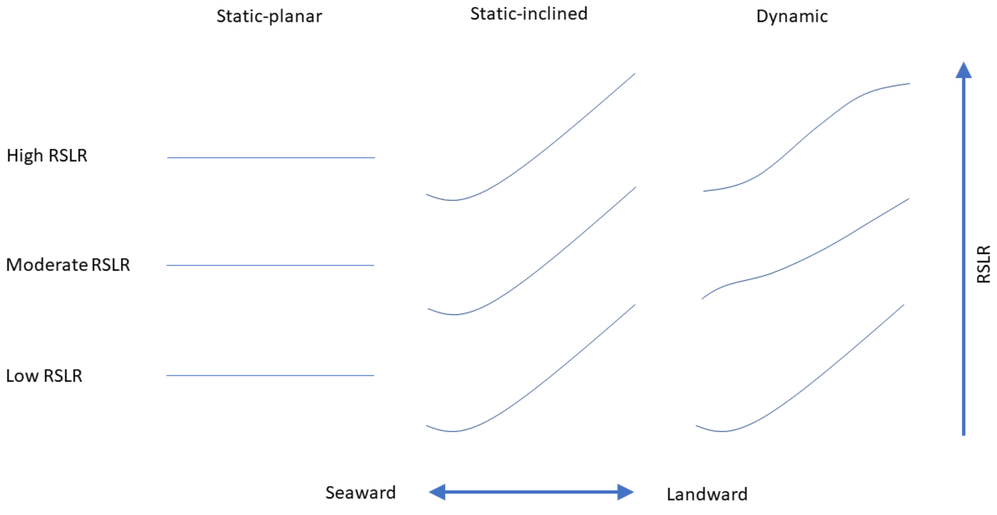
  • To compare the performance of static and dynamic models for assessing coastal flooding exposure to relative sea-level rise (RSLR). Static models extrapolate a fixed water-surface elevation in space to identify land of lower elevation with potential for coastal flooding—the effects of RSLR are assessed via linear addition of RSLR increments to that water surface. Static models are a relative simplification. Dynamic models use detailed hydrodynamic models to simulate the overland flow of water in a physically realistic way—RSLR scenarios are simulated separately to account for the dynamic effects of RSLR. Our comparison of static and dynamic models adds to a body of literature from several cases studies assessing the implications of coastal-flood modelling method on coastal-flood hazard assessments [29,30,31,32,33,34,35,36].
  • To compare the impacts of incremental RSLR on the gradual transition of exposed land area, number and replacement value of buildings and building flood depths from three coastal hazards drivers: coastal flooding during extreme storm-tides, permanent inundation and erosion. This is important because different hazards have different implications for future RSLR adaptation yet are commonly treated in isolation and to our knowledge these three hazards have not been compared together elsewhere. Whereas frequent nuisance or rare but extreme coastal flooding can be tolerated by some communities at present-day MSL [25,46,47], RSLR will increase the frequency of presently large but rare coastal flooding events. Regular coastal flooding or permanent inundation of built land is likely to cause adaptive action [48]. Likewise, coastal erosion removes the land surface, forcing a permanent land-use change [13,49]. Therefore, it may be possible to incrementally adapt to one hazard, but earlier transformational adaptation may be required for another hazard, with RSLR. Overlaying information from multiple hazards resolved in both space and time (here using RSLR as a surrogate for time) can show which hazards will have more impact, where and when.
Therefore, in this paper we quantify the impact of RSLR on the exposed land area, number and replacement value of buildings and building flood depths. Impacts from three coastal hazards were assessed: (1) coastal flooding during extreme storm-tides, (2) permanent inundation and (3) coastal erosion. Section 2 outlines the methods used, including the individual hazard and RSLR scenarios modelled, Section 3 presents the results, Section 4 provides discussion and Section 5 conclusions.

2. Materials and Methods

2.1. Study Location

We model the effects of future sea-level rise on the exposure of land and impacts on buildings inside Tauranga Harbour. Tauranga Harbour is a large, micro-tidal, barrier-enclosed estuarine lagoon, located on the northeast coast of the North Island in New Zealand (Figure 1). Urban development boarders the harbour coastline, including the Tauranga City urban area. Tauranga City has a resident population of 136,713 [50] and operates New Zealand’s largest coastal port by export volume. A previous national assessment of building exposure to 1% AEP coastal flooding in 2016 estimates 953 (NZD$0.3 billion) buildings in Tauranga City could be exposed to coastal flooding at present day MSL [45]. This increases to 2509 (NZD$0.8 billion) and 4124 (NZD$1.4 billion) coastal-flood exposed buildings for a 0.5–1.3 m SLR range expected over the next 100 years in the New Zealand region [28]. In response to these future coastal hazard issues for Tauranga City, coastal flood and erosion hazard modelling was commissioned by a local government partnership who will use the information in regulatory processes such as adaptation policy for regulation of land subdivision and building development [51], to help plan for adaptation to RSLR [52] and to educate landowners of potential risks [53].
Large coastal flooding events in Tauranga Harbour have occurred historically during ex-tropical cyclones in 1936, 1954, 1968 and 2018 and observations include digital sea-level records, supplemented by post-event surveys based on eye-witness accounts [54,55]. The 2018 event was a moderate storm surge combined with an exceptionally high tide, which is the prevalent cause of coastal flooding in New Zealand [18]. Observations of sea level, runup and overland flooding during the 2018 event were used to calibrate the hydrodynamic model [56].

2.2. Hazard-Event and Climate-Change Scenarios

We consider the impacts of three coastal hazards: (1) coastal flooding during extreme storm-tides, (2) permanent inundation, (3) coastal erosion, both now at present-day MSL and after increments of RSLR (Table 1 and Table 2). In this study, present day MSL is considered to be 0.13 m above the local vertical datum Moturiki Vertical Datum 1953 for the baseline year 2020 [57]. Details of the permanent inundation and coastal flooding assessment methods are given in Section 2.3, coastal erosion assessment methods in Section 2.4 and impact modelling in Section 2.5.
The zone of permanent inundation indicates definite continuous impact. The coastal flooding assessments represent a zone of probability: e.g., 1% or 20% AEP. The likelihoods of either a 1% or 20% AEP event occurring within a decade are 10% and 86%, which can respectively be considered “very unlikely” to “likely” [58]. The coastal erosion assessment at the majority of sites within the harbour (with cliffs) represent a zone of vulnerability: e.g., and Ehigh, Emedium represents the distance reached by 66% of all Monte Carlo erosion simulations and Ehigh represents the distance reached by only the largest 5% of erosion simulations (Section 2.4).

2.3. Coastal Flood Modelling and Mapping

2.3.1. Permanent Inundation

Permanent inundation will occur if the land becomes “swallowed” by rising RSLR. In New Zealand, the intersection of the mean high-water springs (MHWS) elevation with the land defines the landward jurisdictional boundary of the coastal marine area [59,60], so we mark the zone of permanent inundation by identifying the area seaward of the line of MHWS. MHWS was calculated as the tidal height equaled or exceeded only by the largest 7% of all high tides and thus exceeded every 14 days on average.

2.3.2. Coastal Flooding

New Zealand guidance recommends identifying zones of “potential” impact from a 1% AEP storm-tide event [52]—a 1% AEP event is equivalent to a 100-year average recurrence interval (or return period) event—this provides an extreme scenario to help with avoidance of risk [28,39]. Owing to their rarity (at present MSL), 1% AEP events are recoverable for many communities through insurance-funded rebuild.
We also estimated the impacts from a more frequent 20% AEP coastal flooding likelihood to represent an expected adaptation tipping point [23,40,61] that would almost certainly necessitate some form of adaptive action before it was reached in Tauranga Harbour. An adaptation tipping point is the point at which a particular action is no longer adequate for meeting a plan’s objectives [40,62,63]. Continual repair of frequently damaged buildings is unlikely to be sustained and thus represents an adaptation tipping point to be avoided if possible—Keenan and Bradt [64] observed that current and anticipated impacts of climate change are shaping the behavior of local real estate markets, particularly within coastal property markets and that banks should be sensitive to climate change effects on their mortgage portfolio risk. A recent report based on anecdotal evidence from the insurance industry suggests that insurance retreat will have occurred by the time this reaches 5% AEP [65]. Consideration of a 20% AEP coastal flood allows a reasonable comparison with the timing of impacts in response to RSLR of coastal erosion and permanent inundation in that each of these scenarios would necessitate adaptive action.
We did not explicitly model the 20% AEP scenario, but a 1% AEP storm-tide at present-day MSL is equivalent to a 20% AEP storm-tide plus a 0.14 m increment of RSLR, which is the elevation difference between a 1% and 20% AEP storm-tide (Figure 2) based on the present-day extreme storm-tide distribution from the Moturiki (Figure 1) sea-level gauge. Therefore, we inferred 20% AEP coastal-flood impacts from the modelled 1% AEP impacts by estimating that 1% AEP impacts would reach 20% AEP frequency after an additional 0.14 m RSLR. Therefore, the minimum RSLR for which 20% AEP flood results are available is 0.14 m.

2.3.3. Coastal Flood and Permanent Inundation Modelling

Coastal flood modelling can be done in several ways, using simple static (“bathtub”) or complex fully dynamic or semi dynamic models, with comparative trade-offs between effort, speed and accuracy [29,30,31,32,33,34,35,36]. The impacts of coastal flooding were assessed using three methods listed in order of decreasing complexity (Figure 3):
  • Dynamic model—a hydrodynamic model individually run for each scenario in Table 2.
  • Static inclined—static GIS-based mapping using the spatially-varying water surface at the shoreline obtained from the hydrodynamic model run using present-day MSL (0 m RSLR) and with the increments of RSLR in Table 2 subsequently added to the spatially-varying water surface.
  • Static planar—static GIS-based mapping using a planar water surface representing the sea level measured at a sea-level recorder within the harbor and with the increments of RSLR in Table 2 subsequently added to the planar water surface.
Static planar models, often referred to “bathtub” models, are operable in a GIS environment and calculate DEM raster cells at topographical elevations below a corresponding sea level elevation [31]. These models support computationally efficient simulations of coastal flooding or permanent inundation caused by sea levels across a range of geographical scales. Static planer model limitations for representing the physical processes that cause coastal flooding are well understood and often result in overestimation of built-asset exposure to flooding [32,33,36]. Ramirez and Lichter [32] found that the most important physical processes not accounted for in static models are: (1) the conservation of mass for flows [66], (2) the effect of landscape roughness on the spread of floodwater and (3) the attenuation of storm-tide by vegetation [67]. These processes generally limit the extent of storm-tide flooding and are needed to replicate flooding in low-lying, topographically flat, vegetated regions. Additionally, static models assume that flood propagation is only limited by topography and that maximum storm-tide water levels are maintained for an infinite duration. Dynamic models overcome the limitations of the static model by simulating the physical processes related to storm-tide flooding [32].
We use the terms static and dynamic to indicate the type of model used to determine the depth, extent and impact of coastal flooding across the floodplain and not to differentiate hydrodynamic forcing conditions driving the flooding, hydrodynamic forcing was similar for all three methods—they are all based on measured or modelled storm-tide. Some studies [68,69] have used the terminology static and dynamic to describe differences in the hydrodynamic forcing conditions, with static used to describe the storm-tide (tide + storm surge) elevations (sometimes referred to as the still-water level) and the term dynamic used to describe the addition of breaking wave effects to the storm-tide. These studies show that including wave effects increases the coastal flood impact in areas where waves are an important flood driver [36].
The two static methods work by comparing a static (inclined or planar) water surface with a digital terrain model (DTM) of the land surface. Areas of the DTM that are below the water surface are assumed to be flooded and the depth and extent of flooding evaluated. In our analysis we removed “ponded” areas from the static flooding maps, these being inland pockets of low-elevation land that are unconnected with the sea and which do not have a known connection via a drain or culvert. For the static-planar method a single water level was expanded across the DTM as a planar surface (Figure 3). For the static-inclined method the spatially variable water surface at the shoreline obtained from the hydrodynamic model simulation at 0 m RSLR was interpolated over the floodplain of the DTM using spline interpolation (Figure 3). The static-inclined flood mapping used the dynamic model simulation of MHWS tide and 1% AEP storm-tide at present-day MSL to obtain a spatially varying surface, to which were subsequently added constant-in-space vertical RSLR increments. Both static methods therefore assume a linear relationship between RSLR and flooding depth.
The hydrodynamic modelling used a calibrated Delft3d hydrodynamic model forced by tidal water levels, river flows, wind and air pressure (inverse barometer effect). A full description of the model setup, calibration, validation and application is provided by Reeve, Stephens [56]. The model used a flexible mesh with a spatial resolution for populated areas of approximately 15 m cell edge length. The model simulated the dynamic evolution of storm-tide around the entire harbour shoreline and dynamically mapped the overland flow path of the water, using a 30 s timestep with results output at 20-min intervals. Since a separate hydrodynamic simulation was run for each RSLR increment, the dynamic model includes non-linear interactions between RSLR and flooding depth and extent. The model’s ability to simulate overland flooding was validated to within a few centimetres of observed elevations against post-flood surveys from the 5 January 2018 storm-tide event [56].
The hydrodynamic modelling of a 1% AEP storm-tide event showed water-level amplification of about 1 m height from the lower harbour to the upper reaches of the harbour sub-inlets. Such storm-tide amplification was observed during the 5 January 2018 storm-tide and observations show that the tide (in absence of surge) also amplifies in the upper reaches of the harbour. Therefore, we expect the static-planar method to give different results to the static-inclined and dynamic-model methods. Further, since the static-planar model was based on water levels derived from a sea-level gauge at Tauranga Port in the lower harbour (Figure 1), we expect that the static-planar method might under-predict the flood-hazard exposure in the upper harbour (and perhaps overall) relative to the other methods.
Like other studies that compared static and dynamic models, we do not integrate morphological-change modelling with coastal flood modelling and our flood and inundation modelling assumes that the land surface will remain as at present [30,31,32,33,34,35,36]. This is a reasonable first-order approximation because (as shown later) the land area exposed to coastal erosion is small compared to that affected by coastal flooding and inundation across the broader floodplain so does not greatly affect the comparison between coastal flooding and erosion. Nevertheless, several studies have shown that future morphological changes could interact with hydrodynamics to affect future coastal flooding impact [49,68,70,71,72]. The morphodynamic evolution of tidal inlets like Tauranga Harbour involves feedbacks between the hydrodynamics of tidal currents and wind waves; the erosion, deposition and transport of sediment; and the morphology resulting from the divergence of the sediment transport [73]. RSLR will change the size, shape and location of the intertidal areas and affect the exchange of sediment between different morphological elements within tidal embayments [74]. This lack of account for morphological evolution of the Harbour is a recognized limitation of our study. However, natural land-building processes are already restricted due to urbanization within Tauranga City and the sheltered inner-harbor location means that waves play a relatively small role in coastal flooding [56] so non-linear amplification of wave impacts [75] are reduced. Human modifications to the landscape, such as the building of seawalls, are also not included in our analyses.

2.4. Coastal Erosion Assessment and Mapping

The coastal erosion and instability hazard areas were determined using a stochastic simulation technique [13]. This technique uses a distribution of values for each component to account for expected variation and uncertainty, rather than single values. The components of erosion are then combined by a Monte Carlo technique to produce a stochastic forecast of hazard area. Outputs include a range of potential erosion hazard distances from the present-day shoreline, for current and future timeframes (i.e., 2020, 2080 and 2130) including RSLR scenarios [52] and for two scenarios that represent mid-range and high-end assumptions on background erosion rate and stable slope angle: Emedium and Ehigh (Table 1). The medium and high erosion scenarios arise from analysis of existing long-term erosion trends, short-term erosion potential for unconsolidated sites and geological assessments of cliff-slumping failure angle within Tauranga Harbour. The combination of these independent variables is derived through a Monte Carlo analysis [13,76,77] where Emedium represents the distance landward of the present-day shoreline reached by 66% of all Monte Carlo erosion simulations and Ehigh represents the distance reached by only the largest 5% of erosion simulations. Comparison between the assessed and observed erosion distances show that the crest of most slopes currently lie between the Emedium and Ehigh lines. The coastal erosion methods are further discussed in Shand et al. (2015) and their application to Tauranga Harbour described by Tonkin and Taylor [76].
Coastal erosion and instability hazard areas were calculated for 32 selected sites around the Tauranga Harbour. These sites were selected based on proximity to existing development and included 88 km of coastline (or approximately 34% of the total harbour length). The land area likely to be affected by erosion within the entire harbour was estimated by scaling up the area affected by the ratio of the total harbour shoreline length (262 km) to the land area associated with the built environment as assessed within this study (88 km).

2.5. Impact Modelling and Mapping

Coastal flooding, inundation and erosion hazard impacts on land and buildings were quantified using the “RiskScape” multi-hazard model framework [78]. The modular framework integrates hazard, exposure (i.e., elements-at-risk) and vulnerability information in a software engine to quantify impact risk at national to local scales (Figure 2) [45]. Here, ‘impact’ refers to the magnitude of land and building exposure to hazards. RiskScape quantified impacts for individual hazard scenarios by intersecting raster (i.e., coastal flooding, permanent inundation) or polygon vector (i.e., erosion) layers with land and building polygon vector layers, then calculating geometric units for land and building features located within hazard extents [45]. The impacts from coastal flooding, permanent inundation and coastal erosion were quantified as (1) exposed land area (km2), (2) exposed number and replacement value (NZD$ 2016) of buildings exposed and (3) building exposure to coastal flood depths.

3. Results

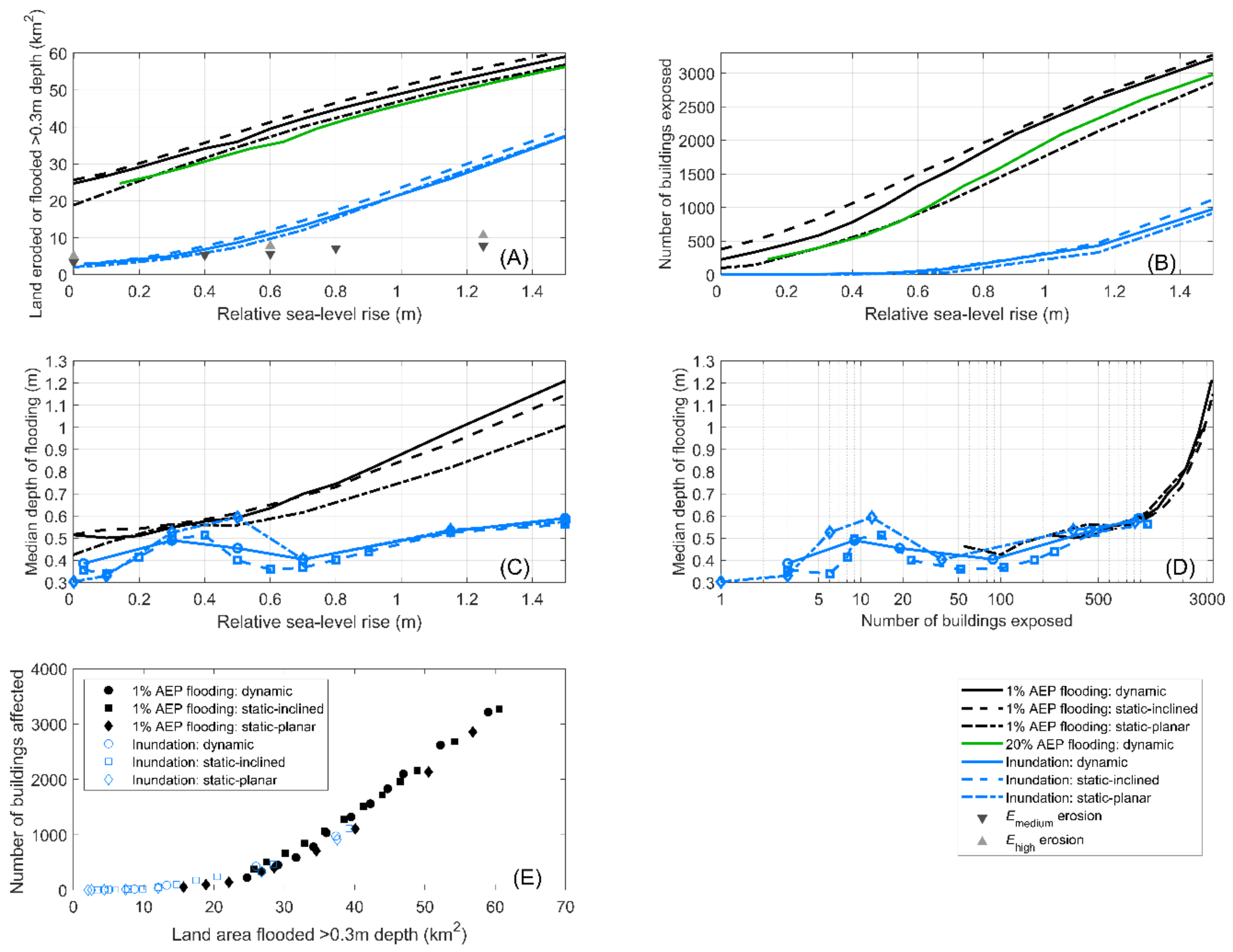
3.1. Coastal Flooding and Inundation Exposure in Tauranga Harbour

The exposure to coastal flooding and permanent inundation will increase as the sea level rises (Figure 4). In this section, we focus on the presenting land and building impacts from the hydrodynamic model—we compare results from the hydrodynamic and static models in Section 3.2.
The hydrodynamic model identified 25 km2 of land already exposed to coastal flooding of ≥0.3 m depth in an extreme 1% AEP sea-level event (Table S1, Figure 4a). This will rise to about 60 km2 at 1.5 m MSL and the increase in exposure is approximately linear with RSLR. Less than 3 km2 of land is already exposed to coastal flooding of ≥0.3 m during MHWS tides, but this will rise to about 37 km2 at 1.5 m MSL. The increase in exposure accelerates for RSLR ≤ 0.7 m RSLR and is approximately linear thereafter (Figure 4a). At present, some 3.3–5 km2 (EmediumEhigh) of land is vulnerable to coastal instability and erosion. This increases to 5.3–7.8 km2 by 2080 with 0.4 to 0.6 m RSLR depending on the scenario selected and to between 7.2–11.3 km2 by 2130.
The dynamic model shows there are presently (at 0 m RSLR) about 230 buildings exposed to coastal flooding in an extreme 1% AEP sea-level event and this will rise to about 3200 buildings at 1.5 m MSL (Figure 4b).
Presently there are no buildings seaward of the line of MHWS, but this will change with RSLR (Figure 4b). The land seaward of the line of MHWS would effectively be “in the sea” from a legal perspective and would experience regular coastal flooding at least every fortnight over the spring tides—thus, representing permanent inundation. The hydrodynamic model shows 19 buildings would be permanently inundated when RSLR reaches 0.5 m, 88 buildings at 0.7 m MSL and almost 1000 buildings at 1.5 m MSL (Figure 4b).
For the 230 buildings presently exposed to the rare chance of a 1% AEP event, the frequency of coastal flooding will increase dramatically in future with RSLR (Figure 5a). We expect those 230 buildings to flood about once every 2 years after 0.2 m RSLR and about 3 times per year after 0.3 m of RSLR, which will occur sometime between 2044–2082 (Table 3). At >0.3 m RSLR those buildings will be flooded many times per year.
After 0.14 m RSLR there would be about 230 buildings exposed to 20% AEP (5-year return-period) coastal flooding and this would rise to about 1000 buildings exposed after about 0.6 m RSLR (Figure 4b). A 0.14 m RSLR is presently the difference between a 1% and 20% AEP storm-tide elevation and is the minimum RSLR for which 20% AEP results are available (see Section 2.3.2).
The median depth of flooding of buildings generally increases with RSLR (Figure 4c). The permanent inundation scenarios show a peak in the median depth of flooding at 0.4–0.6 m RSLR before dropping and a gradual increase after 0.8 m RSLR (Figure 4c). This peak is due to a small number (5–20) buildings being flooded to relatively high median depths by MHWS at 0.4–0.6 m RSLR scenarios, then the median flood depth drops as more buildings become impacted at 0.6–0.8 m RSLR, thereafter increasing beyond about 0.8 m RSLR. Both the number of buildings exposed and the median flooded depth increase with RSLR—hence, the median depth of flooding increases with the total number of buildings exposed (Figure 4d).
The relationship between land area and number of buildings flooded is similar regardless of model type, or the severity of the event (e.g., compare inundation to 1% AEP coastal flooding, Figure 4e). At low RSLR, the land area flooded increases relatively faster than the number of buildings—the number of buildings flooded then accelerates relative to land area—before reaching an approximately linear relationship at large RSLR (Figure 4e).

3.2. Comparing Dynamic, Static-Inclined and Static-Planar Models for Coastal-Flood Modelling

The dynamic, static-inclined and static-planar models gave qualitatively similar results for evaluating the impacts of flooding and permanent inundation from RSLR, i.e., the observed trend of exposure with RSLR is similar but the magnitude of exposure varies between methods (Figure 4). We found the static-planar modelling to underpredict coastal-flood exposure relative to the dynamic and static-inclined methods.
The difference between the static-planar and dynamic model predictions of land and building exposure and total building replacement value (Figure 5b) to coastal flooding was greater for large RSLR, with the dynamic model showing a stronger non-linear response to RSLR than either the static-planar or static-inclined model (Figure 4a,b and Figure 5b).
The static-inclined model was a closer approximation to the dynamic model compared to the static-planar model for exposed land and buildings along with median coastal flooding depth (Figure 4 and Figure 6). Differences between the dynamic and static-inclined models were largest for ≤0.8 m, the models gave similar results above 0.8 m (Figure 4b).

3.3. Comparison of Coastal Flooding and Erosion

In terms of land area affected, permanent inundation will overtake coastal erosion after about 0.4 m RSLR (Figure 4a), which is projected to occur between 2062–2104 (Table 3).
There are about 75 buildings within the present-day Emedium zone exposed to coastal erosion and this will rise to about 640 buildings at 1.5 m RSLR. If erosion is worse than expected (i.e., under the Ehigh scenario) then more than 800 buildings could be affected after 1.5 m RSLR (Table S2, Figure 4c).
At present, MSL 230 buildings lie within the 1% AEP coastal flood exposure, with between 75 (Emedium scenario) to 300 (Ehigh scenario) buildings exposed to coastal erosion. As sea-level starts to rise, coastal flooding will soon affect many more buildings than coastal erosion (Figure 5a).
Comparing coastal flooding and coastal erosion: Figure 5a indicates that coastal erosion could impact more buildings at present-day MSL. However, 20% AEP coastal flooding, recurring every 5 years on average, will affect more buildings than coastal erosion after about 0.15–0.2 m RSLR, which is expected to occur between 2038–2062. After 1.5 m RSLR, which could occur by the year 2135 under a fast RSLR scenario, more buildings will be affected by permanent inundation than by coastal erosion and building exposure to coastal flooding by 20% AEP storm-tides is around 5 times those potentially exposed to coastal erosion.
The relative impacts of coastal flooding, inundation and erosion on total building replacement value are similar to results for number of buildings exposed (Figure 5b). Total building replacement value from a present-day 20% AEP coastal flood event is projected to rise from NZD$104 million after 0.14 m RSLR to >NZD$1200 million after 1.5 m RSLR, whereas maximum total building replacement value from coastal erosion is estimated at NZD$248 million for a high erosion scenario.

3.4. Impact Thresholds

Presently, there is no national assessment of impact-based thresholds for coastal flooding or erosion in New Zealand, nor locally established impact thresholds for Tauranga. For example, the USA has local minor coastal flooding threshold levels established by the U.S. National Oceanic and Atmospheric Administration (NOAA) NWS [25] and impact-based thresholds for coastal flooding were recently defined in Australia [79].
Although there are no established impact-based thresholds, our results enable us to evaluate impacts of RSLR in terms of land area, buildings exposed, replacement value of exposed buildings and median coastal flooding depth (Figure 4 and Figure 5). We can compare the impact thresholds between hazard drivers (coastal flooding, inundation and erosion) and the three model types used to evaluate coastal flooding and inundation.
For example, for an impact threshold of 500 buildings exposed or NZD$200 million total building replacement value (Figure 5) the impact from 20% AEP coastal flooding precedes that of permanent inundation by about 0.8 m RSLR, which equates to 2091–2192 years (Table 3). For RSLR ≥ ~0.3 m, projected impacts from 20% AEP coastal flooding are much larger than those from coastal erosion. Permanent inundation would have similar impact to erosion after 1–1.3 m RSLR.
The static-planar modelling returned up to 18% (484) less buildings impacted (after 1.15 m RSLR) by 1% AEP storm-tides, compared with the dynamic model (Table S2). The static-planar model estimated that 0.2 m more RSLR would be required to reach 1500 buildings impacted by 1% AEP storm-tides, compared with the dynamic model (Figure 4). It will take between 24–42 years for 0.2 m of RSLR to occur depending on whether the RSLR rate is fast or slow (Table 3). Although the static and dynamic results appear qualitatively similar, use of the static-planar model could result in a 1500 building-impact threshold (for example) being reached 24–42 years earlier than planned for, in this case.
Whereas the static-planar model underpredicted hazard exposure, the static-inclined model predicted conservatively high exposure compared with the dynamic model (Figure 4b)—up to 27% (282) more buildings exposed (after 0.5 m RSLR) to a 1% AEP storm-tide and a maximum 0.14 m lower RSLR to reach a specific (500 buildings) threshold exposed to a 1% AEP storm-tide.

4. Discussion

Coastal erosion and 1% AEP coastal flooding events have immediate impact potential at present-day MSL, but the impact from RSLR increases much faster for coastal flooding. For RSLR ≥ 0.2 m, there are large differences between coastal flooding, permanent inundation and erosion, in the RSLR required to reach equivalent impact thresholds (Figure 5). The erosion or permanent inundation of built environments would necessitate adaptive action. Coastal flooding of 20% AEP frequency is also likely to promote some form of adaptive action, via mitigation of flooding impacts [48], or as a response to mortgage lending policies or insurance retreat [65,66]. Based on this premise, for ≥0.2 m RSLR, coastal flooding will have a much bigger impact overall than coastal erosion (Figure 7) and will breach adaptation tipping points for land and building impacts earlier. However, some properties on coastal cliffs could remain safe from flooding but be impacted by erosion so it is important to account for both hazards. In developing plans for adaptation to avoid coastal hazards, adaptation pathways would include different adaptation tipping points that relate to locally relevant actions and triggers for action [39,40,48,62,80,81]. Our results show that increasingly frequent coastal flooding will be the dominant trigger for adaptation in Tauranga, New Zealand. These findings are similar to Dawson and Dickson [49] who found that over the twenty-first century, coastal flood risk on the East Anglian coast of England is expected to be an order of magnitude greater than erosion risk.
Based on guidance for local government when planning for coastal hazard impacts [52], New Zealand’s local and regional governments are using the 1% AEP coastal flood elevation + RSLR to set minimum floor building levels and other planning rules. In some cases, this includes few mapped RSLR scenarios, while in others it includes regular RSLR increments. Of the four hazard metrics we compared, the 1% AEP coastal flooding area encompasses the most land, buildings and has the largest total building replacement value. When planning to avoid future coastal-flooding related impacts for new developments on undeveloped “greenfield” sites, it makes sense to use a relatively large 1% AEP event + large RSLR allowance [28,39]. However, not all land or buildings within the 1% AEP coastal flood area will be subject to the same frequency and magnitude of flooding-related impacts. For existing built environments, more urgent adaptation will be required within the 20% AEP coastal flood and permanent inundation areas, both of which lie within the 1% AEP coastal flood area. In other words, there will be a transition towards larger and increasingly frequent impacts within the 1% AEP area with RSLR. These transition impacts include the effects of rising groundwater and a rapidly increasing frequency of nuisance flooding prior to permanent inundation [25,27,82,83]. The concept of impacts being unequal in space and time within a single hazard zone is not necessarily obvious—land and buildings are shown either as inside or outside the zone and assumed to be inundated/eroded or not inundated/eroded. By considering several hazards, this study helps to show how a gradient of impacts will arise with RSLR—in this case the zones between permanent inundation and 1% AEP coastal flooding provide a zone for the transition of coastal flooding impacts with RSLR. The evaluation of impacts from regular increments of RSLR and several hazard metrics shows the transition of impact thresholds in response to multiple hazards. This nuanced information can be useful when designing adaptive plans to trigger adaptive action not too early or too late [39,40].
In Tauranga, New Zealand, only 0.14 m RSLR separates a frequency change from 1% to 20% AEP coastal flooding and this is similar for other coastal cities in New Zealand [18,23]. A 0.14 m RSLR could occur between 2038–2048 based on New Zealand’s SLR projections (Table 3). Extreme storm-tide distributions and factors of coastal flood-frequency increase with RSLR are similar in New Zealand to many places throughout the world that are also tidally dominant [26,84,85]. Thus, land and buildings within the present-day 1% AEP coastal flood area will experience rapidly increasing coastal flooding frequency with RSLR in many places globally.
The dynamic model, which included the dynamic interaction between storm-tide and incremental RSLR, showed a more nonlinear increase with RSLR in both the number of buildings flooded and median depth of flooding, compared with the static-inclined and static-planar modelling which rely on offsetting a fixed water surface by linear RSLR increments. Our dynamic modelling results support findings that future coastal flooding impacts will not be linearly proportional to the static SLR [71,72]. Like Breilh and Chaumillon [30] and McGrath and Bourgon [34], we found that static-inclined results were better matched than static-planar results, when compared to dynamic model simulations or to observations.
Previous studies have generally found that a static-planar model of storm-tide provides conservatively-high (overpredicts) estimates of coastal flooding area and depth compared with dynamic models or measured storm impacts [29,30,31,32,33,34,35,36], although this is site specific and can vary regionally due to local changes in storm-tide energy and topography [30,33,37]. Differences were found to be greater mainly over large, low flat areas where dynamic effects of friction become important. In contrast, to most other studies, we found the static-planar modelling to underpredict coastal flood exposure over the whole domain, relative to the dynamic and static-inclined methods—this was also observed by Barnard and Erikson [69]. In our case the levels for the static-planar model were obtained from a sea-level gauge in the lower Tauranga harbour where water levels are lower during storm-tide events, because topographic constriction causes the tide and storm surge to amplify within the upper arms of the harbour. In our study the sloping water surface within the harbour during extreme (e.g., 1% AEP) events is an important factor that limits the ability of the static-planar model to accurately represent the hazard exposure. A static-planar model would have performed better where extreme sea-levels were more spatially uniform. The static-planar model could have returned conservatively large exposure had we used a sea-level gauge in the upper harbour to derive higher static-planar water levels and correspondingly would have predicted lower RSLR required to reach exposure thresholds. Thus, the degree of water-level setup during extreme events and the static water level height chosen to represent them is an important consideration when undertaking static-planar modelling.
We observed that a static-planar model underestimates land and building exposure to coastal flooding by up to 2.3 times in the Tauranga urban area, compared to a dynamic model. This finding may indicate that at 0.2 m RSLR national building exposure to 1% AEP coastal flooding events derived from static planar models [45] could be underestimated by ~23,300 buildings (NZD$7.3 billion [45]). In addition, if 0.14–0.2 m RSLR were to reduce a 1% AEP event to a 20% AEP event, nationally ~62,300 buildings (NZD$16.1 billion) would be exposed to coastal flooding every 5 years on average sometime between 2038 and 2062. Future timing of increased coastal flood exposure is, however, dependent on local extreme sea levels and RSLR influenced by factors such as vertical land movement [86] and adaptation interventions, e.g., flood protection structures. Despite their higher resource requirements relative to static models, dynamic model application, particularly within coastal urban areas, would better account for the absolute coastal flooding exposure of built land and assets, along with timing of exposure in response to RSLR [69].

5. Conclusions

We quantified the impact of RSLR on the exposed land area, number and replacement value of buildings and building flood depths next to Tauranga Harbour, New Zealand. Impacts were assessed from three coastal hazards: (1) coastal flooding during extreme storm-tides, (2) permanent inundation and (3) coastal erosion. Comparison of the three hazards highlights a gradient of hazard exposure. The quantification of land and building impacts from small (0.1 m) increments of RSLR shows emerging coastal flood and erosion hazard exposure to facilitate both short-term and long-term land-use management and adaptation planning. We also contrasted the use of dynamic, static-inclined and static-planar (“bathtub”) flood models to determine the impact of coastal flooding and permanent inundation through time as sea level rises.
In terms of total land area, total number of buildings and total replacement value, adaptation tipping points will be reached by frequent (20% AEP) coastal flooding well before permanent inundation or coastal erosion. Increasingly frequent coastal flooding will be the dominant trigger for adaptation in Tauranga, New Zealand. In the absence of adaptation, recurrent coastal flooding, recurring once or more every 5 years on average (i.e., 20% AEP), will overtake erosion as the dominant coastal hazard after about 0.15–0.2 m RSLR, which is likely to occur between years 2038–2062 in New Zealand and will rapidly escalate in frequency and consequence thereafter. Coastal erosion will remain the dominant hazard for property on high-elevation coastal cliffs. It will take about 0.8 m more RSLR for permanent inundation to reach the same impact thresholds as 20% AEP coastal flooding, in terms of land area exposed and number and replacement value of buildings affected.
The areas of permanent inundation and 1% and 20% AEP coastal flooding enable to visualize the transition of coastal flooding impacts with RSLR. We found that impacts within the subsequent decade presently associated with ‘very unlikely’ 1% AEP coastal flooding will transition to ‘likely’ 20% AEP after only 0.14 m RSLR, so the 1% AEP coastal flood area signals 20% AEP coastal flooding within 0.14 m RSLR, which provides 2–3 decades (18–28 years) “lead-in” time, depending on the RSLR rate, to a (20% AEP coastal flooding) situation that we expect will necessitate prior adaptive action.
Dynamic, static-inclined and static-planar models gave qualitatively similar results for evaluating the impacts of coastal flooding and permanent inundation from RSLR. However, the static-planar modelling indicated up to 18% less buildings impacted by 1% AEP storm-tides and up to 0.2 m more RSLR required to impact an equivalent number of buildings, compared with the dynamic model that simulates non-linear impacts of RSLR. Use of the static-planar model could result in sea level thresholds being reached 24–42 years earlier than planned for in this case. This is compelling evidence to use dynamic models to support adaptation planning.

Supplementary Materials

The following are available online at https://www.mdpi.com/article/10.3390/jmse9091011/s1, Figure S1: Photograph of a coastal landslip in Omokoroa within Tauranga Harbour. Figure S2: Flooding of low-lying coastal land during the high storm-tide on 5 February 2018. Figure S3: Flooding of low-lying coastal land during the high storm-tide on 5 February 2018. Figure S4: High tide at the Bay St Reserve which borders the Matua Estuary on 17 November 2016. Table S1: Land area flooded to a depth ≥0.3 m. Table S2: Total number of buildings exposed to coastal flooding, permanent inundation and coastal erosion. Table S3: Total building replacement value. Table S4: Median depth of flooding of buildings. Table S5: Estimate of land area affected from coastal erosion.

Author Contributions

Conceptualization, S.A.S. and R.P.; methodology, R.P., G.R., S.W., T.S.; formal analysis, S.A.S., G.R., S.W., B.P., R.H.; writing—original draft preparation, S.A.S.; writing—review and editing, R.P.; visualization, G.R., S.W., R.H.; funding acquisition, S.A.S. All authors have read and agreed to the published version of the manuscript.

Funding

The research was funded by the New Zealand Ministry of Business, Innovation and Employment (MBIE) under (a) the Natural Hazard Research Platform Climate Change Impacts on Weather-Related Hazards project 3710440 and (b) Strategic Science Investment Fund (Project CAVA2104—National Institute of Water and Atmospheric Research). Writing of the paper was provided in part through the Coastal Programme of the Resilience to Nature’s Challenges Kia Manawaroa—Ngā Akina o Te Ao Tūroa, contract GNS-RNC040—Coastal. The coastal erosion and coastal flood modelling was commissioned by partnership of Councils and the modelling studies were co-designed with Council staff: Western Bay of Plenty District Council (Tony Clough), Tauranga City Council (Campbell Larking) and Bay of Plenty Regional Council (Mark Ivamy and Peter Blackwood). Willem de Lange from University of Waikato and Mark Dickson from University of Auckland provided peer review on the modelling design and reporting.

Institutional Review Board Statement

Not applicable.

Informed Consent Statement

Not applicable.

Data Availability Statement

Data is available online from supporting studies: https://atlas.boprc.govt.nz/api/v1/edms/document/A3338785/content, accessed on 12 August 2021 and https://www.tauranga.govt.nz/Portals/0/data/living/natural_hazards/files/harbour_erosion_assessment.pdf, accessed on 12 August 2021, and within the Supplementary Materials.

Conflicts of Interest

The authors declare no conflict of interest.

References

  1. Hallegatte, S.; Green, C.; Nicholls, R.; Corfee-Morlot, J. Future flood losses in major coastal cities. Nat. Clim. Chang. 2013, 3, 802–806. [Google Scholar] [CrossRef]
  2. Brown, S.; Nicholls, R.; Hanson, S.; Brundrit, G.; Dearing, J.; Dickson, M.E.; Gallop, S.; Gao, S.; Haigh, I.D.; Hinkel, J.; et al. Shifting perspectives on coastal impacts and adaptation. Nat. Clim. Chang. 2014, 4, 752–755. [Google Scholar] [CrossRef]
  3. Haigh, I.D.; Ozsoy, O.; Wadey, M.P.; Nicholls, R.; Gallop, S.L.; Wahl, T.; Brown, J. An improved database of coastal flooding in the United Kingdom from 1915 to 2016. Sci. Data 2017, 4, 170100. [Google Scholar] [CrossRef] [Green Version]
  4. Thomas, B.; Bruno, C.; Roshanka, R.; Guy, W.; Jeremy, R.; Nicolas, B.; Déborah, I.; Jessie, L.; Salas-Mélia, D. Quantifying uncertainties of sandy shoreline change projections as sea level rises. Sci. Rep. 2019, 9, 42. [Google Scholar]
  5. Wahl, T.; Brown, S.; Haigh, I.D.; Nilsen, J.E. Øie Coastal Sea Levels, Impacts, and Adaptation. J. Mar. Sci. Eng. 2018, 6, 19. [Google Scholar] [CrossRef] [Green Version]
  6. McMichael, C.; Dasgupta, S.; Ayeb-Karlsson, S.; Kelman, I. A review of estimating population exposure to sea-level rise and the relevance for migration. Environ. Res. Lett. 2020, 15, 123005. [Google Scholar] [CrossRef]
  7. Jongman, B.; Ward, P.J.; Aerts, J.C. Global exposure to river and coastal flooding: Long term trends and changes. Glob. Environ. Chang. 2012, 22, 823–835. [Google Scholar] [CrossRef]
  8. Brown, S.; Nicholls, R.J.; Goodwin, P.; Haigh, I.D.; Lincke, D.; Vafeidis, A.T.; Hinkel, J. Quantifying Land and People Exposed to Sea-Level Rise with No Mitigation and 1.5 °C and 2.0 °C Rise in Global Temperatures to Year 2300. Earth’s Future 2018, 6, 583–600. [Google Scholar] [CrossRef]
  9. Kulp, S.A.; Strauss, B.H. New elevation data triple estimates of global vulnerability to sea-level rise and coastal flooding. Nat. Commun. 2019, 10, 4844. [Google Scholar] [CrossRef] [PubMed] [Green Version]
  10. Bruun, P. Sea-Level Rise as a Cause of Shore Erosion. J. Waterw. Harb. Div. 1962, 88, 117–130. [Google Scholar] [CrossRef]
  11. Walkden, M.; Dickson, M. Equilibrium erosion of soft rock shores with a shallow or absent beach under increased sea level rise. Mar. Geol. 2008, 251, 75–84. [Google Scholar] [CrossRef]
  12. Thiéblemont, R.; Le Cozannet, G.; Rohmer, J.; Toimil, A.; Álvarez-Cuesta, M.; Losada, I.J. Deep uncertainties in shoreline change projections: An extra-probabilistic approach applied to sandy beaches. Nat. Hazards Earth Syst. Sci. 2021, 21, 2257–2276. [Google Scholar] [CrossRef]
  13. Cowell, P.J.; Thom, B.G.; Jones, R.A.; Everts, C.H.; Simanovic, D. Management of uncertainty in predicting climate-change impacts on beaches. J. Coast. Res. 2006, 22, 232–245. [Google Scholar] [CrossRef]
  14. Ashton, A.D.; Walkden, M.J.; Dickson, M.E. Equilibrium responses of cliffed coasts to changes in the rate of sea level rise. Mar. Geol. 2011, 284, 217–229. [Google Scholar] [CrossRef]
  15. Gutierrez, B.T.; Plant, N.G.; Thieler, E.R. A Bayesian network to predict coastal vulnerability to sea level rise. J. Geophys. Res. Space Phys. 2011, 116, 15. [Google Scholar] [CrossRef] [Green Version]
  16. Ray, R.D.; Foster, G. Future nuisance flooding at Boston caused by astronomical tides alone. Earth’s Future 2016, 4, 578–587. [Google Scholar] [CrossRef]
  17. Haigh, I.D.; Wadey, M.P.; Wahl, T.; Ozsoy, O.; Nicholls, R.; Brown, J.; Horsburgh, K.; Gouldby, B. Spatial and temporal analysis of extreme sea level and storm surge events around the coastline of the UK. Sci. Data 2016, 3, 160107. [Google Scholar] [CrossRef] [PubMed] [Green Version]
  18. Stephens, S.A.; Bell, R.G.; Haigh, I.D. Spatial and temporal analysis of extreme storm-tide and skew-surge events around the coastline of New Zealand. Nat. Hazards Earth Syst. Sci. 2020, 20, 783–796. [Google Scholar] [CrossRef] [Green Version]
  19. Hinkel, J.; Lincke, D.; Vafeidis, A.; Perrette, M.; Nicholls, R.; Tol, R.; Marzeion, B.; Fettweis, X.; Ionescu, C.; Levermann, A. Coastal flood damage and adaptation costs under 21st century sea-level rise. Proc. Natl. Acad. Sci. USA 2014, 111, 3292–3297. [Google Scholar] [CrossRef] [PubMed] [Green Version]
  20. Nicholls, R.J.; Marinova, N.; Lowe, J.A.; Brown, S.; Vellinga, P.; de Gusmão, D.; Hinkel, J.; Tol, R.S.J. Sea-level rise and its possible impacts given a ‘beyond 4 °C world’ in the twenty-first century. Philos. Trans. R. Soc. A Math. Phys. Eng. Sci. 2011, 369, 161–181. [Google Scholar] [CrossRef] [PubMed] [Green Version]
  21. Church, J.A.; Clark, P.U.; Cazenave, A.; Gregory, J.M.; Jevrejeva, S.; Levermann, A.; Merrifield, M.A.; Milne, G.A.; Nerem, R.S.; Nunn, P.D.; et al. Sea Level Change. In Climate Change 2013: The Physical Science Basis. Contribution of Working Group I to the Fifth Assessment Report of the Intergovernmental Panel on Climate Change; Stocker, T.F., Qin, D., Plattner, G.-K., Tignor, M., Allen, S.K., Boschung, J., Nauels, A., Xia, Y., Bex, V., Midgley, P.M., Eds.; Cambridge University Press: Cambridge, UK; New York, NY, USA, 2013; pp. 1137–1216. [Google Scholar]
  22. Karegar, M.A.; Dixon, T.H.; Malservisi, R.; Kusche, J.; Engelhart, S. Nuisance Flooding and Relative Sea-Level Rise: The Importance of Present-Day Land Motion. Sci. Rep. 2017, 7, 11197. [Google Scholar] [CrossRef] [PubMed] [Green Version]
  23. A Stephens, S.; Bell, R.; Lawrence, J. Developing signals to trigger adaptation to sea-level rise. Environ. Res. Lett. 2018, 13, 104004. [Google Scholar] [CrossRef]
  24. Vitousek, S.; Barnard, P.L.; Fletcher, C.H.; Frazer, N.; Erikson, L.; Storlazzi, C.D. Doubling of coastal flooding frequency within decades due to sea-level rise. Sci. Rep. 2017, 7, 1399. [Google Scholar] [CrossRef]
  25. Sweet, W.V.; Park, J. From the extreme to the mean: Acceleration and tipping points of coastal inundation from sea level rise. Earth’s Future 2014, 2, 579–600. [Google Scholar] [CrossRef]
  26. Hunter, J. A simple technique for estimating an allowance for uncertain sea-level rise. Clim. Chang. 2011, 113, 239–252. [Google Scholar] [CrossRef]
  27. Dahl, K.A.; Spanger-Siegfried, E.; Caldas, A.; Udvardy, S. Effective inundation of continental United States communities with 21st century sea level rise. Elem. Sci. Anth. 2017, 5, 37. [Google Scholar] [CrossRef] [Green Version]
  28. Stephens, S.A.; Bell, R.G.; Lawrence, J. Applying Principles of Uncertainty within Coastal Hazard Assessments to Better Support Coastal Adaptation. J. Mar. Sci. Eng. 2017, 5, 40. [Google Scholar] [CrossRef]
  29. Bates, P.D.; Dawson, R.J.; Hall, J.W.; Horritt, M.S.; Nicholls, R.J.; Wicks, J.; Hassan, M.A.A.M. Simplified two-dimensional numerical modelling of coastal flooding and example applications. Coast. Eng. 2005, 52, 793–810. [Google Scholar] [CrossRef]
  30. Breilh, J.F.; Chaumillon, E.; Bertin, X.; Gravelle, M. Assessment of static flood modeling techniques: Application to contrasting marshes flooded during Xynthia (western France). Nat. Hazards Earth Syst. Sci. 2013, 13, 1595–1612. [Google Scholar] [CrossRef] [Green Version]
  31. Seenath, A.; Wilson, M.; Miller, K. Hydrodynamic versus GIS modelling for coastal flood vulnerability assessment: Which is better for guiding coastal management? Ocean Coast. Manag. 2016, 120, 99–109. [Google Scholar] [CrossRef]
  32. Ramirez, J.A.; Lichter, M.; Coulthard, T.J.; Skinner, C. Hyper-resolution mapping of regional storm surge and tide flooding: Comparison of static and dynamic models. Nat. Hazards 2016, 82, 571–590. [Google Scholar] [CrossRef]
  33. Didier, D.; Baudry, J.; Bernatchez, P.; Dumont, D.; Sadegh, M.; Bismuth, E.; Bandet, M.; Dugas, S.; Sévigny, C. Multihazard simulation for coastal flood mapping: Bathtub versus numerical modelling in an open estuary, Eastern Canada. J. Flood Risk Manag. 2018, 12, e12505. [Google Scholar] [CrossRef]
  34. McGrath, H.; Bourgon, J.-F.; Proulx-Bourque, J.-S.; Nastev, M.; El Ezz, A.A. A comparison of simplified conceptual models for rapid web-based flood inundation mapping. Nat. Hazards 2018, 93, 905–920. [Google Scholar] [CrossRef]
  35. Kumbier, K.; Carvalho, R.C.; Vafeidis, A.T.; Woodroffe, C.D. Comparing static and dynamic flood models in estuarine environments: A case study from south-east Australia. Mar. Freshw. Res. 2019, 70, 781. [Google Scholar] [CrossRef]
  36. Vousdoukas, M.I.; Voukouvalas, E.; Mentaschi, L.; Dottori, F.; Giardino, A.; Bouziotas, D.; Bianchi, A.; Salamon, P.; Feyen, L. Developments in large-scale coastal flood hazard mapping. Nat. Hazards Earth Syst. Sci. 2016, 16, 1841–1853. [Google Scholar] [CrossRef] [Green Version]
  37. Hagen, S.C.; Bacopoulos, P. Coastal flooding in Florida’s Big Bend Region with application to sea level rise based on synthetic storms analysis. Terr. Atmos. Ocean Sci. 2012, 23, 481–500. [Google Scholar] [CrossRef] [Green Version]
  38. Minister of Conservation. New Zealand Coastal Policy Statement 2010; D.o.C. Publishing Team, Ed.; Department of Conservation: Wellington, New Zealand, 2010; p. 38.
  39. Lawrence, J.; Bell, R.; Blackett, P.; Stephens, S.; Allan, S. National guidance for adapting to coastal hazards and sea-level rise: Anticipating change, when and how to change pathway. Environ. Sci. Policy 2018, 82, 100–107. [Google Scholar] [CrossRef]
  40. Haasnoot, M.; Kwakkel, J.H.; Walker, W.E.; ter Maat, J. Dynamic adaptive policy pathways: A method for crafting robust decisions for a deeply uncertain world. Glob. Environ. Chang. 2013, 23, 485–498. [Google Scholar] [CrossRef] [Green Version]
  41. Lawrence, J.; Bell, R.; Stroombergen, A. A Hybrid Process to Address Uncertainty and Changing Climate Risk in Coastal Areas Using Dynamic Adaptive Pathways Planning, Multi-Criteria Decision Analysis & Real Options Analysis: A New Zealand Application. Sustainability 2019, 11, 406. [Google Scholar]
  42. Lawrence, J.; Haasnoot, M. What it took to catalyse uptake of dynamic adaptive pathways planning to address climate change uncertainty. Environ. Sci. Policy 2017, 68, 47–57. [Google Scholar] [CrossRef]
  43. Hunter, J. Estimating sea-level extremes under conditions of uncertain sea-level rise. Clim. Chang. 2009, 99, 331–350. [Google Scholar] [CrossRef]
  44. Kopp, R.E.; Horton, R.M.; Little, C.M.; Mitrovica, J.X.; Oppenheimer, M.; Rasmussen, D.J.; Strauss, B.H.; Tebaldi, C. Probabilistic 21st and 22nd century sea-level projections at a global network of tide-gauge sites. Earth’s Future 2014, 2, 383–406. [Google Scholar] [CrossRef]
  45. Paulik, R.; Stephens, S.; Bell, R.; Wadhwa, S.; Popovich, B. National-Scale Built-Environment Exposure to 100-Year Extreme Sea Levels and Sea-Level Rise. Sustainability 2020, 12, 1513. [Google Scholar] [CrossRef] [Green Version]
  46. Ezer, T.; Atkinson, L.P. Accelerated flooding along the U.S. East Coast: On the impact of sea-level rise, tides, storms, the Gulf Stream, and the North Atlantic Oscillations. Earth’s Future 2014, 2, 362–382. [Google Scholar] [CrossRef]
  47. Moftakhari, H.R.; AghaKouchak, A.; Sanders, B.F.; Allaire, M.; Matthew, R.A. What Is Nuisance Flooding? Defining and Monitoring an Emerging Challenge. Water Resour. Res. 2018, 54, 4218–4227. [Google Scholar] [CrossRef]
  48. Barnett, J.; Graham, S.; Mortreux, C.; Fincher, R.; Waters, E.; Hurlimann, A. A local coastal adaptation pathway. Nat. Clim. Chang. 2014, 4, 1103–1108. [Google Scholar] [CrossRef]
  49. Dawson, R.J.; Dickson, M.E.; Nicholls, R.; Hall, J.W.; Walkden, M.J.A.; Stansby, P.K.; Mokrech, M.; Richards, J.; Zhou, J.G.; Milligan, J.; et al. Integrated analysis of risks of coastal flooding and cliff erosion under scenarios of long term change. Clim. Chang. 2009, 95, 249–288. [Google Scholar] [CrossRef] [Green Version]
  50. Statistics New Zealand. Tauranga City 2018 Census Data. 2018. Available online: https://www.stats.govt.nz/tools/2018-census-place-summaries/tauranga-city (accessed on 12 August 2021).
  51. New Zealand Government. Resource Management Act 1991. Available online: https://www.legislation.govt.nz/act/public/1991/0069/latest/DLM230265.html (accessed on 12 August 2021).
  52. MfE. Coastal Hazards and Climate Change: Guidance for Local Government; Bell, R.G., Ed.; Ministry for the Environment Publication ME1341: Wellington, New Zealand, 2017; 279p. Available online: https://environment.govt.nz/publications/coastal-hazards-and-climate-change-guidance-for-local-government (accessed on 12 August 2021).
  53. TVNZ. Television New Zealand 1 News Online, Over 5000 Tauranga Property Owners Receive Warning Their Homes Are Located in Potential Flood Zone. Available online: https://www.tvnz.co.nz/one-news/new-zealand/over-5000-tauranga-property-owners-receive-warning-their-homes-located-in-potential-flood-zone? (accessed on 12 August 2021).
  54. Gibb, J.G. Review of minimum sea flood levels for Tauranga Harbour. In Report Prepared for Tauranga District Council; C.R. 97/3; Jeremy G. Gibb: Tauranga, New Zealand, 1997; 49p, Available online: https://books.google.com.au/books/about/Review_of_Minimum_Sea_Flood_Levels_for_T.html?id=aGTUvQEACAAJ&redir_esc=y (accessed on 12 August 2021).
  55. De Lange, W.P.; Gibb, J.G. Seasonal, interannual, and decadal variability of storm surges at Tauranga, New Zealand. N. Z. J. Mar. Freshw. Res. 2000, 34, 419–434. [Google Scholar] [CrossRef]
  56. Reeve, G.; Stephens, S.A.; Wadhwa, S. Tauranga Harbour Inundation Modelling. NIWA Client Report 2018269HN to Bay of Plenty Regional Council. 2019; p. 127. Available online: https://atlas.boprc.govt.nz/api/v1/edms/document/A3338785/content (accessed on 12 August 2021).
  57. Stephens, S.A. Tauranga Harbour Extreme Sea Level Analysis. NIWA Client Report to Bay of Plenty Regional Council. 2017; 47p. Available online: https://www.tauranga.govt.nz/Portals/0/data/living/natural_hazards/files/niwa_sea_level_analysis_report.pdf (accessed on 12 August 2021).
  58. Mastrandrea, M.D.; Field, C.B.; Stocker, T.F.; Edenhofer, O.; Ebi, K.L.; Frame, D.J.; Held, H.; Kriegler, E.; Mach, K.J.; Matschoss, P.R.; et al. Guidance Note for Lead Authors of the IPCC Fifth Assessment Report on Consistent Treatment of Uncertainties. Intergovernmental Panel on Climate Change (IPCC). Available online: http://www.ipcc.ch (accessed on 12 August 2021).
  59. Stephens, S.A.; Bell, R.; Ramsay, D.; Goodhue, N. High-Water Alerts from Coinciding High Astronomical Tide and High Mean Sea Level Anomaly in the Pacific Islands Region. J. Atmos. Ocean. Technol. 2014, 31, 2829–2843. [Google Scholar] [CrossRef]
  60. Baker, R.F.; Watkins, M. Guidance Notes for the Determination of Mean High Water Mark for Land Title Surveyors. In Kearns, Kerr and Smith (1997) Chapter 5 Law for Surveyors—Boundaries and Boundary Definition, Dept of Surveying University of Otago/NZIS Available from School of Surveying, University of Otago; Professional Development Committee of the New Zealand Institute of Surveyors: Dunedin, New Zealand, 1991. [Google Scholar]
  61. Haasnoot, M.; Schellekens, J.; Beersma, J.J.; Middelkoop, H.; Kwadijk, J.C.J. Transient scenarios for robust climate change adaptation illustrated for water management in The Netherlands. Environ. Res. Lett. 2015, 10, 105008. [Google Scholar] [CrossRef] [Green Version]
  62. Kwadijk, J.C.J.; Haasnoot, M.; Mulder, J.P.M.; Hoogvliet, M.M.C.; Jeuken, A.B.M.; van der Krogt, R.A.A.; van Oostrom, N.G.C.; Schelfhout, H.A.; van Velzen, E.H.; van Waveren, H.; et al. Using adaptation tipping points to prepare for climate change and sea level rise: A case study in the Netherlands. Wiley Interdiscip. Rev. Clim. Chang. 2010, 1, 729–740. [Google Scholar] [CrossRef]
  63. Werners, S.; Pfenninger, S.; van Slobbe, E.; Haasnoot, M.; Kwakkel, J.; Swart, R. Thresholds, tipping and turning points for sustainability under climate change. Curr. Opin. Environ. Sustain. 2013, 5, 334–340. [Google Scholar] [CrossRef]
  64. Keenan, J.M.; Bradt, J.T. Underwaterwriting: From theory to empiricism in regional mortgage markets in the U.S. Clim. Chang. 2020, 162, 2043–2067. [Google Scholar] [CrossRef]
  65. Storey, B.; Sigma, C.; Owen, S.; Noy, I.; Zammit, C. Insurance Retreat: Sea level rise and the withdrawal of residential insurance in Aotearoa New Zealand. In Report for the Deep South National Science Challenge; NZ Deep South Science Challenge: Wellington, New Zealand, 2020. [Google Scholar]
  66. De Almeida, G.A.M.; Bates, P.; Freer, J.E.; Souvignet, M. Improving the stability of a simple formulation of the shallow water equations for 2-D flood modeling. Water Resour. Res. 2012, 48, W05528. [Google Scholar] [CrossRef]
  67. Gedan, K.B.; Kirwan, M.L.; Wolanski, E.; Barbier, E.B.; Silliman, B.R. The present and future role of coastal wetland vegetation in protecting shorelines: Answering recent challenges to the paradigm. Clim. Chang. 2011, 106, 7–29. [Google Scholar] [CrossRef]
  68. Barnard, P.L.; Erikson, L.H.; Foxgrover, A.C.; Hart, J.A.F.; Limber, P.; O’Neill, A.C.; Van Ormondt, M.; Vitousek, S.; Wood, N.; Hayden, M.K.; et al. Dynamic flood modeling essential to assess the coastal impacts of climate change. Sci. Rep. 2019, 9, 4309. [Google Scholar] [CrossRef] [PubMed] [Green Version]
  69. Storlazzi, C.D.; Berkowitz, P.; Reynolds, M.H.; Logan, J.B. Forecasting the Impact of Storm Waves and Sea-Level Rise on Midway Atoll and Laysan Island within the Papahānaumokuākea Marine National Monument—A Comparison of Passive Versus Dynamic Inundation Models; U.S. Geological Survey: Reston, VA, USA, 2013; p. 83.
  70. Bilskie, M.V.; Hagen, S.C.; Alizad, K.; Medeiros, S.C.; Passeri, D.L.; Needham, H.F.; Cox, A. Dynamic simulation and numerical analysis of hurricane storm surge under sea level rise with geomorphologic changes along the northern Gulf of Mexico. Earth’s Future 2016, 4, 177–193. [Google Scholar] [CrossRef] [Green Version]
  71. Ding, Y.; Kuiry, S.; Elgohry, M.; Jia, Y.; Altinakar, M.S.; Yeh, K.-C. Impact assessment of sea-level rise and hazardous storms on coasts and estuaries using integrated processes model. Ocean Eng. 2013, 71, 74–95. [Google Scholar] [CrossRef]
  72. Lentz, E.E.; Thieler, E.R.; Plant, N.G.; Stippa, S.R.; Horton, R.; Gesch, D.B. Evaluation of dynamic coastal response to sea-level rise modifies inundation likelihood. Nat. Clim. Chang. 2016, 6, 696–700. [Google Scholar] [CrossRef]
  73. De Swart, H.; Zimmerman, J. Morphodynamics of Tidal Inlet Systems. Annu. Rev. Fluid Mech. 2009, 41, 203–229. [Google Scholar] [CrossRef]
  74. Van Maanen, B.; Seiffert, R.; Rasquin, C.; Kösters, F. Modeling the morphodynamic response of tidal embayments to sea-level rise. Ocean Dyn. 2013, 63, 1249–1262. [Google Scholar] [CrossRef]
  75. Arns, A.; Dangendorf, S.; Jensen, J.; Talke, S.; Bender, J.; Pattiaratchi, C. Sea-level rise induced amplification of coastal protection design heights. Sci. Rep. 2017, 7, 40171. [Google Scholar] [CrossRef]
  76. Tonkin & Taylor. Tauranga Harbour Coastal Hazards Study: Coastal Erosion Assessment. Report 1001628.v5 to Bay of Plenty Regional Council July 2019. Available online: https://www.tauranga.govt.nz/Portals/0/data/living/natural_hazards/files/harbour_erosion_assessment.pdf (accessed on 12 August 2021).
  77. Shand, T.; Reinen-Hamill, R.; Kench, P.; Ivamy, M.; Knook, P.; Howse, B. Methods for Probabilistic Coastal Erosion Hazard Assessment. In Proceedings of the Australasian Coasts & Ports Conference 2015, Auckland, New Zealand, 15–18 September 2015. [Google Scholar]
  78. Schmidt, J.; Matcham, I.; Reese, S.; King, A.; Bell, R.; Henderson, R.; Smart, G.; Cousins, J.; Smith, W.; Heron, D. Quantitative multi-risk analysis for natural hazards: A framework for multi-risk modelling. Nat. Hazards 2011, 58, 1169–1192. [Google Scholar] [CrossRef]
  79. Hague, B.S.; Murphy, B.F.; Jones, D.A.; Taylor, A.J. Developing impact-based thresholds for coastal inundation from tide gauge observations. J. South Hemisph. Earth Syst. Sci. 2019, 69, 252–272. [Google Scholar]
  80. Haasnoot, M.; van’t Klooster, S.; van Alphen, J. Designing a monitoring system to detect signals to adapt to uncertain climate change. Glob. Environ. Chang. 2018, 52, 273–285. [Google Scholar] [CrossRef]
  81. Kwakkel, J.H.; Haasnoot, M.; Walker, W.E. Developing dynamic adaptive policy pathways: A computer-assisted approach for developing adaptive strategies for a deeply uncertain world. Clim. Chang. 2014, 132, 373–386. [Google Scholar] [CrossRef] [Green Version]
  82. Befus, K.M.; Barnard, P.L.; Hoover, D.J.; Hart, J.A.F.; Voss, C.I. Increasing threat of coastal groundwater hazards from sea-level rise in California. Nat. Clim. Chang. 2020, 10, 946–952. [Google Scholar] [CrossRef]
  83. Rotzoll, K.; Fletcher, C.H. Assessment of groundwater inundation as a consequence of sea-level rise. Nat. Clim. Chang. 2012, 3, 477–481. [Google Scholar] [CrossRef]
  84. Merrifield, M.A.; Genz, A.S.; Kontoes, C.P.; Marra, J.J. Annual maximum water levels from tide gauges: Contributing factors and geographic patterns. J. Geophys. Res. Oceans 2013, 118, 2535–2546. [Google Scholar] [CrossRef]
  85. Rueda, A.; Vitousek, S.; Camus, P.; Tomás, A.; Espejo, A.; Losada, I.J.; Barnard, P.L.; Erikson, L.H.; Ruggiero, P.; Reguero, B.G.; et al. A global classification of coastal flood hazard climates associated with large-scale oceanographic forcing. Sci. Rep. 2017, 7, 5038. [Google Scholar] [CrossRef]
  86. Denys, P.H.; Beavan, R.J.; Hannah, J.; Pearson, C.F.; Palmer, N.; Denham, M.; Hreinsdottir, S. Sea Level Rise in New Zealand: The Effect of Vertical Land Motion on Century-Long Tide Gauge Records in a Tectonically Active Region. J. Geophys. Res. Solid Earth 2020, 125, e2019JB018055. [Google Scholar] [CrossRef]
Figure 1. Location of Tauranga Harbour, New Zealand, also showing the Tauranga City urban area boundary and the location of the Moturiki Island tide gauge outside the Harbour and the Tauranga Port tide gauge within the lower Harbour.
Jmse 09 01011 g001
Figure 2. Upper plot: extreme sea-level distribution from the Moturiki Island (Figure 1) sea-level gauge. Lower plot: Increase in the number (N) of sea-level events per year reaching or exceeding the present-day 1% annual exceedance probability (AEP) elevation, with relative sea-level rise. The lower plot saturates at 706 high tides per year all exceeding the present-day 1% AEP sea-level elevation.
Jmse 09 01011 g002
Figure 3. Schematic of water surface elevation changes applied within the three coastal-flood-modelling methods.
Jmse 09 01011 g003
Figure 4. Coastal flooding, permanent inundation and erosion exposure in Tauranga Harbour with relative sea-level rise: (A) RSLR versus land area exposed to ≥0.3 m coastal flood depth, (B) RSLR versus number of buildings exposed to coastal flooding and inundation, (C) RSLR versus median depth of coastal flooding, (D) number of buildings exposed versus median depth of coastal flooding and (E) Relationship between land area and number of buildings flooded.
Jmse 09 01011 g004
Figure 5. (A) Comparison of hydrodynamic model-derived building exposure to an “extreme” 1% AEP sea-level, 20% AEP sea-level and a typical high spring tide, for RSLR up to 1.5 m above present. In addition, shown are the Emedium and Ehigh coastal erosion scenarios and the increase in the annual expected number of exceedances (N) of the present-day 1% AEP elevation; (B) RSLR versus the building replacement value exposed.
Jmse 09 01011 g005
Figure 6. Comparison of model types for 1% AEP coastal flooding + 0.4 m RSLR, at a port storage facility in Tauranga Harbour. Red = dynamic, purple = static-planar, hashed = static-inclined.
Jmse 09 01011 g006
Figure 7. Comparison of hazard exposure extent for an area within Tauranga Harbour: (A) RSLR = 0.4 m, (B) RSLR = 0.6 m.
Jmse 09 01011 g007
Table 1. Coastal erosion scenarios modelled. RSLR in metres relative to present-day MSL.
Timeframe in YearsRSLR Scenario (m)Erosion Scenario
Present-day (2020)0.0Emedium, Ehigh
20800.4Emedium
0.6Emedium, Ehigh
21300.8Emedium
1.25Emedium, Ehigh
1.6Ehigh
Table 2. Coastal flooding and inundation scenarios modelled. RSLR in metres relative to present-day MSL. Timing for RSLR scenarios is provided in Table 3.
Coastal Flooding/Inundation ScenariosSea-Level Rise Scenarios (m)
MHWS (permanent inundation)0, 0.1, 0.2, …, 1.0, 1.15, 1.5
1% AEP storm-tide (coastal flooding)0, 0.1, 0.2, …, 1.0, 1.15, 1.5
20% AEP storm-tide (coastal flooding)=1% AEP + 0.14 m + RSLR scenarios
Table 3. Approximate years, from possible earliest to latest, when specific sea-level rise increments (metres above 2020 MSL) could be reached for various projection scenarios of sea-level rise for the wider New Zealand region (adapted from [28,52]).
RSLRNZ RCP2.6 M (Median)NZ RCP4.5 M (Median)NZ RCP8.5 M (Median)NZ H+
02020202020202020
0.12040203820372033
0.142048204620432038
0.22062205720512044
0.32082207320632054
0.42104208920742062
0.52126210520832070
0.62148212120922077
0.72170213621002084
0.82192215021072091
0.92215216521152097
1.02238217821232104
1.12261219221312111
1.22285220521402117
1.32309221821482123
1.42334223121532129
1.52359224421592135
Publisher’s Note: MDPI stays neutral with regard to jurisdictional claims in published maps and institutional affiliations.

