A Decision Support Tool for Long-Term Planning of Marine Operations in Ocean Energy Projects

Abstract

Ocean energy is a relevant source of clean renewable energy, and as it is still facing challenges related to its above grid-parity costs, tariffs intended to support in a structured and coherent way are of great relevance and potential impact. The logistics and marine operations required for installing and maintaining these systems are major cost drivers of marine renewable energy projects. Planning the logistics of marine energy projects is a highly complex and intertwined process, and to date, limited advances have been made in the development of decision support tools suitable for ocean energy farm design. The present paper describes the methodology of a novel, opensource, logistic and marine operation planning tool, integrated within DTOceanPlus suite of design tools, and responsible for producing logistic solutions comprised of optimal selections of vessels, port terminals, equipment, as well as operation plans, for ocean energy projects. Infrastructure selection logistic functions were developed to select vessels, ports, and equipment for specific projects. A statistical weather window model was developed to estimate operation delays due to weather. A vessel charter rate modeling approach, based on an in-house vessel database and industry experience, is described in detail. The overall operation assumptions and underlying operating principles of the statistical weather window model, maritime infrastructure selection algorithms, and cost modeling strategies are presented. Tests performed for a case study based a theoretical floating wave energy converter produced results in good agreement with reality.

1. Introduction

The decarbonization of the energy sector is urgent, requiring global action to achieve our long-term climate goals and to mitigate the impacts of climate change [1]. To meet our ambitious emission cuts, innovation in low-carbon technologies and mass deployment of renewable energy generation will be fundamental [2,3].

As a renewable energy resource, ocean energy is clean, abundant, and powerful. Wave and tidal energy are attractive sources of renewable energy, as they have low variability when compared to wind, can be accurately forecast, and are fit to respond to the electricity demand during night-time [4]. Additionally, the production profile of wave and tidal energy systems is complementary to wind and solar, smoothing the otherwise peaking nature of renewables in the production mix [5]. It is estimated that about 100 GW of wave and tidal energy capacity can be deployed in Europe by 2050 [6], creating significant carbon emission reductions as well as economic growth opportunities. Europe’s seas and oceans could therefore play a fundamental role in the decarbonization of the energy sector, contributing to the transition from a power system based on imported fossil fuels, to a flexible and interconnected system based on clean, renewable, and infinite domestic resources [7]. However, the ocean energy sector is still facing challenges related to performance, reliability, and survivability, which ultimately translates into above grid-parity costs.

Logistics and marine operations are major cost drivers of marine renewable energy projects. Even though researchers have made significant progress over the last years in what concerns the installation and operation and maintenance (O&M) planning of offshore wind farms [8,9,10,11], advances for ocean energy farms have been more modest, attesting for the lower maturity of the sector [12]. For offshore wind, the installation costs typically represent one fifth to one third of the project’s CapEX [13,14,15], while O&M activities represent about one-fourth to one-half of the total lifetime costs of the project [16]. However, for less mature sectors such as wave and tidal energy, slightly larger percentages may be expected [17]. These costs are typically amplified when deploying projects in further offshore waters, as the marine operations related to the construction, installation, maintenance, and decommissioning of such farms become increasingly challenging. Even though deploying farms further offshore is expected to improve resource availability and consequently increase the expected power output of the farm (while also minimizing competition for space and visual disturbance [18]), more severe weather climates and larger distances to shore translate into lower farm accessibility, higher risks of work delays, and ultimately larger project costs. As a significant fraction of the marine operation costs can be attributed to vessel charter (according to Dalgic et al. [19], approximately 73% of the total O&M costs are related to vessel hiring [19]), even modest reductions in operation duration may result in significant cost-reductions [20].

Planning the logistics of offshore renewable projects is a highly intertwined process, with multiple conflicting objectives and alternatives, and a large optimization potential. Given the complexity associated with planning such logistics, computational tools have been developed to support decision-making at different project stages. Computational tools can be distinguished according to (i) decision-making time-scale (long-term strategic planning based on historical weather data, or short-term daily operational planning based on weather forecasts), (ii) project phase (installation, O&M, and decommissioning), (iii) target sector (offshore wind, ocean energy, or both), (iv) licensing type (open-source, private, or commercial), and (v) software functionalities (e.g., weather window modeling, operation planning, infrastructure selection, failure/degradation modeling, revenue modeling, and techno-economic assessments).

Table 1. Examples of logistic support tools for marine renewable energy projects, featuring their functionalities. Tools were labeled according to their capabilities, namely, to select suitable infrastructure solutions in respect to ports (P), vessels (V), and equipment (E).

Organisation	Product Name	Open Source	Applicable to Ocean Energy	Weather Window Analysis	Infra- Structure Selection	Optimal Operation Plan	Inst	O&M	Decom.
DNV-GL	O2M	No	No	Hindcast	No	No	No	Yes	No
DNV-GL	OMCAM	No	No	Hindcast	No	No	No	Yes	No
ECN	ECN O&M Access	No	No	Forecast	No	No	No	Yes	No
DTOcean 1.0 /2.0	DTO Logistics module [26,27]	Yes	Yes	Hindcast	P, V, E	Yes	Yes	Yes	No
DTOceanPlus	DTO+ LMO module	Yes	Yes	Hindcast	P, V, E	Yes	Yes	Yes	Yes
ECN (TNO)	ECN O&M Calculator (OMCE) [28]	No	No	Hindcast	No	No	No	Yes	No
Fraunhofer IWES	Multi-Agent-System	No	No	Hindcast	No	No	No	Yes	No
ROMEO	ROMEO O&M Tool [29]	N/A	No	Forecast	No	No	No	Yes	No
SINTEF Energy Research	NoWIcob [30]	No	No	Hindcast	V	No	No	Yes	No
SINTEF Ocean (MARINTEK)	Vessel fleet optimization models [31,32]	No	No	Hindcast	V	No	No	Yes	No
Shoreline	Shoreline Design [33]	No	No	Hindcast	No	No	Yes	Yes	No
Strathclyde University	StrathOW-OM [34,35]	No	No	Hindcast	No	No	No	Yes	No
EDF Group	ECUME-I [36,37]	No	No	Hindcast	No	No	No	Yes	No
Wave Energy Scotland	WES O&M Tool [38]	Yes	Yes	Hindcast	No	No	No	Yes	No
James Fisher and Sons	Mermaid [23]	No	Agnostic	Hindcast	No	No	-	-	-
JBA Consulting	ForeCoast Marine [24]	No	Agnostic	Hindcast	No	No	-	-	-
StormGEO	StormGEO S-Planner [25]	No	Agnostic	Forecast	No	No	-	-	-

shows a list of the main logistic support tools developed to date with the goal of supporting offshore projects. It can be seen that most development efforts have focused on producing O&M simulation tools to estimate the OPEX of offshore wind projects. Some of these tools were developed to simulate the degradation of farm components and the occurrence of failures, replicating real-world decisions in respect to the scheduling of preventive and corrective maintenance activities [21]. This is the case of ECN O&M Tool, the ECN O&M Calculator (formerly OMCE) and the O2M model of DNV-GL [22]. As most operations carried out at sea are significantly weather dependent, computational tools generally include weather window models to estimate the potential waiting on weather contingencies. Some commercial and sector-agnostic tools, such as Mermaid [23] and ForeCoast Marine [24] (marked as ”Agnostic” in Table 1), have focused almost exclusively on this type of service, quantifying weather risks for different operation types and target sectors. Another similar commercial product worth mentioning is StormGeo [25], which also provides short-term decision support based on near-future weather forecasts.

However, it is possible to observe that very limited advances have been made in the development of logistic support tools suitable for ocean energy farm design. Existing computational tools either focus exclusively on the O&M phase (e.g., WES O&M Tool [38]) or are limited in functionality. A reduced number of tools has been developed to address vessel selection in offshore wind projects (e.g., NOWICOB [30] and StrathOW-OM [35]). Still, these tools do not consider the selection of ports and equipment (nor their impacts on optimal vessel selection), and most importantly, are not easily adaptable to ocean energy projects [39]. Moreover, most existent tools are notably user input-intensive, and thus unsuitable for project and technology developers at early development stages where uncertainties and unknowns are large. Finally, despite the growing number of open-source initiatives, which have been found to contribute significantly to sector innovations and to the European Union’s economy [40,41], most computational tools were developed under private or commercial licenses with limited published research. As such, these tools miss out on the key benefits of open-source projects, related to higher transparency, robustness and scrutiny, as well as continuous improvements through community collaborations.

At a project development phase, integrating preliminary plans for the installation, maintenance, and decommissioning in the design process has the potential to reveal unexpected impacts of certain component design decisions on logistic costs. This is a particularly important step for ocean energy projects as less mature technologies have higher cost-optimization potential, frequently achievable with simple concept adjustments. In order to address the identified research gaps and market needs, the Logistics and Marine Operations (LMO) module was developed and integrated within DTOceanPlus software, an open-source suite of design tools for ocean energy projects [42]. The LMO module is responsible for designing and planning the project life-cycle phases (i.e., installation, maintenance, and decommissioning) of ocean energy projects. Reflecting the most recent experiences and best practices of the offshore wind sector, the LMO module produces logistic solutions comprised of optimal selections of vessels, port terminals, equipment, as well as operation plans, for ocean energy projects. An innovative methodology to optimize the selection of vessels, port terminals, and equipment was developed. A novel vessel cost modeling methodology was implemented in order to take into consideration the impacts of vessel capabilities on charter price, and reveal cost reduction pathways. Comprehensive, purpose-built databases of offshore operations, vessels, ports, and equipment were generated to support the main functionalities of the tool, even when unknowns are large and data availability is limited. These databases will be made freely available upon the final release of the DTOceanPlus software. Leveraging on its main functionalities, the Logistics and Marine Operations module proposes optimal logistic solutions that minimize total project costs, guiding project design and strategic investment decisions in ocean energy projects at different stages of technological and project maturity.

The present paper describes in detail the novel Logistics and Marine Operations tool, one of the seven design modules of the DTOceanPlus software. In Section 2, the DTOcean-Plus software is briefly presented. The underlying operating principle, main functionalities, and methodology of the Logistic and Marine Operations tool are described in detail in Section 3. A brief test case showcasing the functionalities of the DTOceanPlus Logistics module is described in Section 4. The most important outcomes of the work are summarized in Section 5.

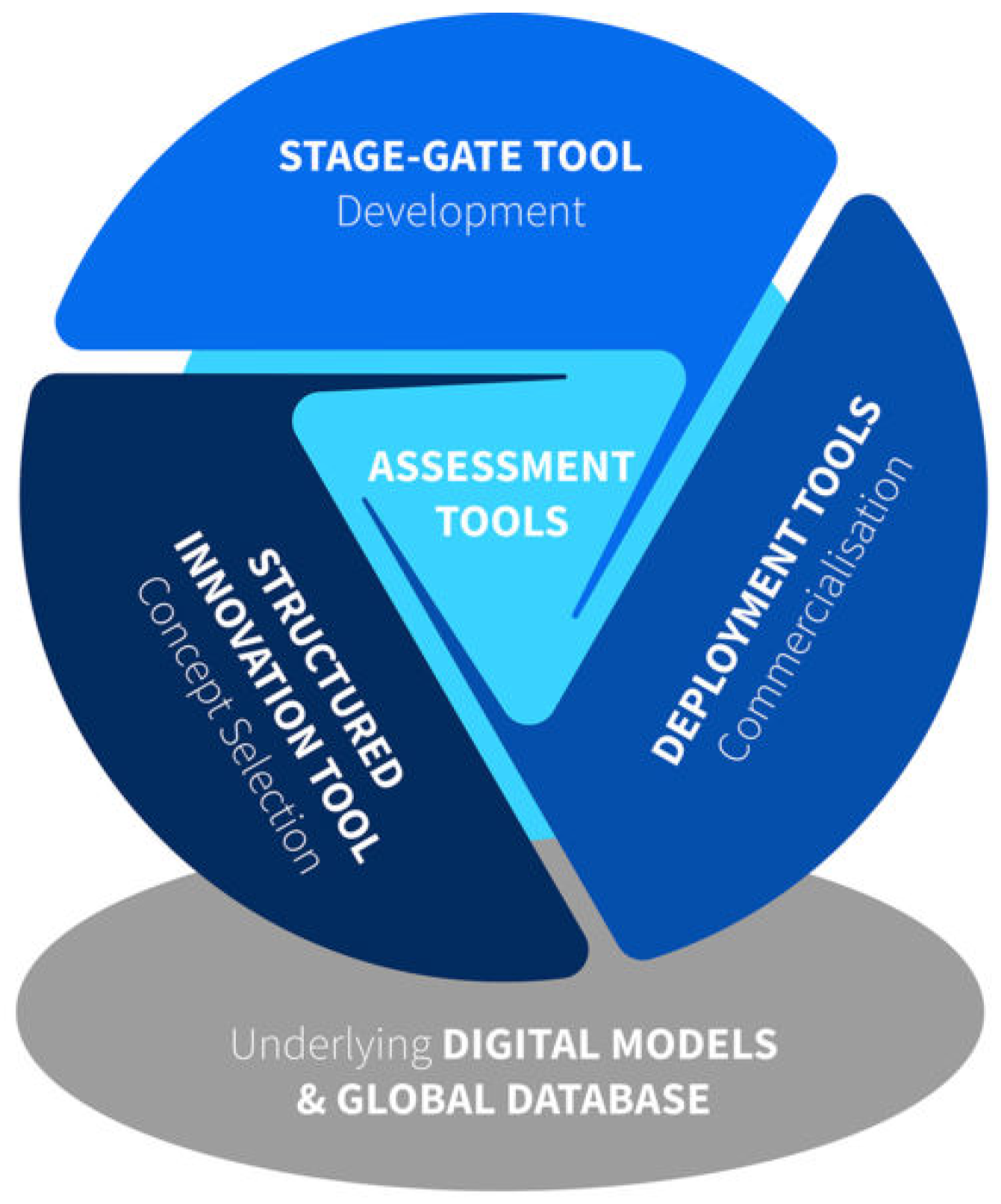
2. DTOceanPlus Suite of Design Tools

DTOceanPlus is an open source, integrated suite of design tools, developed to support the selection, development, deployment, and assessment of ocean energy systems at different stages and levels of aggregation (component, sub-system, and array). Building on the results from the original DTOcean project [43,44,45], at the time of writing, DTOceanplus software is being developed within a 3-years long EU-funded H2020 project with the same name [42], aimed at accelerating the commercialization of the ocean energy sector.

As illustrated in Figure 1, DTOceanPlus was developed in a modular fashion, with a set of independent but integrated tools:

• Structured Innovation tool, to support innovation and the selection of technology concepts;
• Stage Gate tool, to guide technology developers in their technology development process;
• Deployment Design design tools, to support optimal device and array deployment:

  -

  Site Characterization (SC), to characterize the deployment site in respect to environmental (e.g., met-ocean) and geotechnical conditions;

  -

  Machine Characterization (MC), to characterize the device’s prime mover;

  -

  Energy Capture (EC), to design and optimize the device hydrodynamics at an array level;

  -

  Energy Transformation (ET), to design the Power Take-off (PTO) unit and control strategies;

  -

  Energy Delivery (ED), to design the electrical power transmission system of the farm;

  -

  Station Keeping (SK), to produce foundations and mooring designs;

  -

  Logistics and Marine Operations (LMO), to design logistical solutions related to the installation, operation, maintenance, and dismantling operations.

• Assessment design tools, devised to evaluate ocean energy projects in respect to key metrics:

  -

  System Performance and Energy Yield (SPEY), to assess projects in respect to their energy performance;

  -

  System Lifetime Costs (SLC), to assess projects from the economic and financial investment perspectives;

  -

  System Reliability, Availability, Maintainability, Survivability (RAMS), to evaluate different reliability aspects of ocean energy projects;

  -

  Environmental and Social Acceptance (ESA), to evaluate ocean energy projects in respect to their environmental and social impacts.

• Underlying digital models to provide a standard framework for the description of ocean energy sub-systems, as well as a global database with reference data from various sources.

3. Logistics and Marine Operations Module

3.1. Operating Principle

The Logistics and Marine Operation (LMO) module was designed to generate optimal logistical solutions for the installation, O&M, and decommissioning phases of ocean energy projects. These logistic solutions consist of an operation plan (featuring dates and sequence of activities) and an optimal combination of vessels, equipment and ports that minimize the costs of each operation individually, reducing the capital and operational expenditures (CAPEX and OPEX) of the project.

The operating principle behind the LMO module is similar for all three life cycle stages of the project, and can be described as a sequence of different steps, as schematized in Figure 2. First, the LMO module collects design inputs from the user and previously run Deployment design modules (listed in Section 2), data related to the devices and subsystems that must be installed, maintained, and dismantled throughout the lifetime of the project (see Figure 3. More information about the inputs available in [46]). These attributes are subsequently converted into project logistic requirements (e.g., N monopiles with specific dimensions and a given weight need to be lifted, transported, and installed). Second, based on the specified components and identified requirements, the corresponding marine operations that must be carried out are identified (e.g., pile installation). In respect to O&M, two maintenance types are simultaneously considered in the LMO module: preventive (time-based maintenance) and corrective, based on failure events generated by the RAMS module [47] taking into consideration component failure distributions.

In a third step, the process of identifying feasible infrastructure solutions begins. Vessels, ports, and equipment must not only meet their minimum individual prerequisites imposed by the project, but also be compatible between each other. Then, for each potential logistic solution, defined by a specific operation plan and infrastructure setup, the operation net durations and expected waiting on weather (WOW) are computed based on historical weather data and a operation catalog, featuring reference operation durations and weather restrictions (e.g., maximum wave height and maximum wind speed). Following the calculation of the total operation durations (including weather delays), for each logistic solution, the operation total costs can be calculated by considering the daily costs of the infrastructure setup. Finally, the logistic solution that presents the lowest operation total costs can be chosen as the optimal solution.

In the DTOceanPlus software suite, each module was developed with three levels of complexity (Cpx1, Cpx2, and Cpx3) to accommodate different stages of project maturity, and different amounts of data availability and uncertainties. In LMO, the main differences between complexity Cpx2 and Cpx3 are the certainty of the inputs and whether default values are assumed instead of requesting these from the user. Alternatively, the simplified mode (Cpx1) can be used for early stage technologies, at lower technology readiness levels (TRL 1-3), or whenever limited information is available about the technology design and project specifics. The simplified mode may also be used to provide a quick and rough estimate for higher TRL projects. Finally, a “study comparison” feature was implemented in DTOceanPlus to enable the user to evaluate and compare different inputs, strategies, and scenarios, in respect to their impacts on the logistic solutions.

In order to carry out the design of the installation, maintenance, and decommissioning phases, the LMO module employs databases of vessels, port terminals and operations, that will be publicly available once the final version of the DTOceanPlus suite of tools is released.

3.2. Compilation of Operations and Logistic Requirements

In a first step, the Logistics and Marine Operations module reads component design inputs generated by previously run DTOceanPlus Deployment Design modules and/or introduced by the user. Based on the specified component designs, number of components, and user preferences, the LMO module identifies and proposes to the user a list and sequence of operations to install, service and/or dismantle a given ocean energy farm (see

Table 2. List of operations for each project phase included in the Logistics and Marine Operations module.

Installation Operations	Maintenance Operations	Decommissioning Operations
Foundations installation	Topside inspection	Device removal
Moorings installation	Underwater inspection	Collection point removal
Support structures installation	Mooring inspection	Moorings removal
Collection point installation	Array cable inspection	Foundations removal
Export cable installation	Export cable inspection
Array cable installation	Device retrieval
Post-lay cable burial	Device repair at port
External protection installation	Device redeployment
Device installation	Device repair on site
	Mooring line replacement
	Array cable replacement1
	Export cable repair

for the list of operations considered in LMO). For each operation, relevant operational methods (e.g., transportation method and piling method) are read from upstream modules (e.g., cable burial layout is generated by the Energy Delivery module, using specific cable burial methods), or requested to the user, as described in

Table 3. Operation methods considered in the LMO module.

Method List	Defined by	Options
Transportation	User	Dry	Wet	-	-
Port load-out	User/Default	Lift	Float	Skidded	Railed
Cable burial	User/ED module	Ploughing	Jetting	Cutting	-
Burial sequence	User/Default	Simultaneous	Post-lay	-	-
Cable landfall	User/Default	OCT	HDD	-	-
Piling	User/Default	Hammering	Vibro-piling	Drilling	-

.

Based on the identified operations and specified operation methods, infrastructure requirements are defined (e.g., the vessel’s deck area must be sufficient to transport at least one device or system). Infrastructure requirements are compiled in

Table 4. Infrastructure requirements considered in the LMO module.

#	Port Terminal	Vessel	Piling Equipment	Cable Burial Equipment	ROV Equipment	Divers
1	Terminal type	Crane capacity	Depth rating	Depth rating	Depth rating	Depth rating
2	Terminal draught	Vessel draft	Pile sleeve diameter	Burial depth	ROV class	-
3	Terminal area	Bollard pull	Penetration depth	Cable diameter	-	-
4	Onshore crane capacity	DP class	Soil type	Cable MBR	-	-
5	Quay soil strength	Deck area	-	-	-	-
6	Max. distance to site	Deck strength	-	-	-	-
7	Past experience	Max. cargo	-	-	-	-
8	-	Turntable storage	-	-	-	-
9	-	Turntable capacity	-	-	-	-
10	-	Max. no. passengers	-	-	-	-

.

3.3. Infrastructure Pre-Selection

3.3.1. Feasible Infrastructure

On a first stage, feasibility functions are used to assess whether vessels, ports and equipment, listed in the DTOceanPlus catalogs, meet the absolute minimum requirements for the job (e.g., sufficient vessel deck area, adequate terminal dry dock dimensions, acceptable ROV depth rating, etc.). These functions are simple mathematical Boolean formulations that filter out the maritime infrastructure noncomplying with the previously defined logistic requirements (see Section 3.2). A default safety factor of 10% is implemented in the feasibility functions to reflect uncertainties and account for potential margins of of error, although this value may be modified by the user.

The identification of feasible ports and equipment follows a simple elimination process, where instances of the port terminals and equipment databases are discarded based on the operation requirements. The port terminal database consists of 203 terminals, from 12 different EU countries, with 21 parameters, including name, type, country, location, terminal entrance width, draught, maximum load, and terminal area, to name a few (see

Table 5. Example port terminal entry of the DTOceanPlus port catalog.

Terminal Parameter	Value
Terminal id	T114
Name of Port	Viana do Castelo
Terminal name	Dry dock #1
Country	Portugal
Terminal coordinates (lat, lon)	(41.675, −8.8383)
Experience in MRE projects	TRUE
Storage area [m2]	100,000
Slipway	TRUE
Terminal type	Dry-dock
Terminal width [m]	32
Terminal length [m]	203
Quay load bearing capacity [t/m2]	0.8
Terminal draught [m]	3.5
Terminal area [m2]	6500
Terminal hinterland area [m2]	3300
Gantry crane lift capacity [t]	80
Tower crane lift capacity [t]	200
Jack-up suitability	TRUE

). Similarly, six main types of equipment (e.g., cable burial tools, piling hammers, and ROVs, to name a few) are considered in DTOceanPlus and included in the equipment catalogs. However, the fleet selection process is slightly more complex.

3.3.2. Fleet Selection Methodology

There are numerous approaches to conduct a given offshore operation. Devices may be transported from port to site, on deck of a large crane vessel with adequate cranes to carry out the installation procedures. Alternatively, they may be loaded at port onto a transport barge, which would in turn be towed a set of tugs or a Anchor Handling Tug and Supply (AHTS) vessel. In case devices were structurally designed for the purpose, they may be individually wet-towed directly to site. Low draft floating converters may be transported using a semi-submersible vessel, with the capability of ballasting down and submerging its deck to unload the converter in the water. Based on the existing experience in the offshore renewable energy sector, a vessel combination (VC) database was developed, namely, for the device installation operation (see

Table 6. Example vessel combinations for the device installation operation, stored in the DTOceanPlus Vessel Combinations catalog.

Id	Type	Transportation	Qty	Main Vessel	Qty	Tow Vessel	Qty	Support Vessel
VC_001	Device Installation	On deck	1	Propelled crane vessel	-	-	-	-
VC_002	Device Installation	On deck	1	Jack-up Vessel	-	-	-	-
VC_003	Device Installation	On deck	1	SOV Gangway	-	-	-	-
VC_004	Device Installation	On deck	1	AHTS	-	-	-	-
VC_005	Device Installation	Dry tow	1	Non propelled crane Vessel	1	Tug	-	-
VC_006	Device Installation	Dry tow	1	Transport Barge	1	Tug	-	-
VC_007	Device Installation	On deck	1	Semi-submersible	-	-	1	Multicat
VC_008	Device Installation	Wet tow	-	-	1	AHTS	-	-
VC_009	Device Installation	Wet tow	-	-	2	AHTS / Tug	-	-
VC_010	Device Installation	Wet tow	-	-	1	AHTS / Tug	1	Multicat
VC_011	Device Installation	Wet tow	-	-	2	AHTS / Tug	1	Multicat
VC_012	Device Installation	Wet tow	-	-	3	AHTS / Tug	1	Multicat

), featuring combinations of different vessel types in different quantities and under different roles. For simplicity, for each vessel combination, three major vessel roles were defined, with different evaluation criteria:

• Main vessels: vessels that play a central role in the operation, being responsible for key activities such as lifting and transporting components, driving a monopile, and installing a cable, to name a few. These vessels are thus assessed in respect to their main attributes (e.g., deck area, crane capabilities, etc.) depending on the vessel type and operation plan.
• Tow vessels: vessels that are responsible for towing a device/structure (wet tow), or a non-propelled barge (dry tow). Tow vessels are assessed in terms of their bollard pull capabilities, which must be sufficiently large to meet the estimated bollard pull requirements for safely towing an object or barge.
• Support vessels: vessels that can be used to support lifts, control marine traffic, and assist device positioning, but do not have a central role in the operation itself.

The fleet selection algorithm follows a two-stage elimination process. It starts by discarding unsuitable vessel combinations that do not meet project requirements or user preferences (e.g., wet tow is not allowed). Then, for each feasible vessel combination, the fleet selection algorithm searches in a vessel cluster database for vessels that meet the technical requirements associated with the attributed roles (e.g., sufficient deck area, sufficient bollard pull to wet tow the device). A given vessel is deemed “feasible” if capable of performing the minimum work criteria (e.g., in case of on deck transportation, vessel must have sufficient deck area to accommodate at least one device per trip).

In DTOceanPlus, a vessel cluster database was compiled based on the statistical analysis of an original database with 14,847 vessels and 46 technical parameters. The very large size of the original database ensured the representativeness of the considered vessel list, although prohibited directly using it in DTOceanPlus due to data privacy issues and to keep computational requirements manageable. In the vessel cluster database, vessels sharing a large number of similar characteristics were grouped into clusters, using the K-Means unsupervised machine learning algorithm [48]. For each technical parameter of each vessel cluster, the p25, p50, and p75 statistical values were computed and stored. Deliverable D5.8 [46] provides more information about the vessel clustering process.

3.3.3. Infrastructure Matching

Once feasible infrastructure have been identified, infrastructure-matching functions assess the compatibility between each infrastructure type in the context of an integrated solution. In this step, independently feasible but incompatible infrastructure solutions are discarded (e.g., port entrance width must be larger then vessel beam, port draught must be compatible with vessel draft, etc.). Once the infrastructure matching algorithm has been run, suitable infrastructure combinations are produced to be further analyzed in respect to total operation duration and ultimately, costs.

3.4. Definition of Activity Sequence

In the LMO module, operations (e.g., foundation installation) are broken down into smaller, uninterruptible tasks that must be carried out, referred to as activities (e.g., mobilization, transit, and positioning), with specific durations and weather restrictions. For each operation, activity flowcharts were developed, featuring the activity blocks, precedence rules (i.e., which activity comes next), and condition nodes which define multiple potential paths that an operation may take. Condition nodes were defined as static, when based on previously defined component types and operation methods (e.g., foundation type is a pile, transportation method is dry), or dynamic, when dependent on the considered infrastructure solution and operation stage (e.g., vessel is already full or not). In the flowcharts, activities may have a constant duration, or a dynamic duration when the activity length depends on external criteria such as distance and vessel transit speeds (for transits and tows) or soil conditions (e.g., for piling activities such a “Seafloor drilling”). In

Table 7. Flowchart of the foundation installation operation, featuring activity blocks, precedence rules, and condition nodes (shown in italic).

ID	Activity Name	Next Activity	Duration [h]	Decision Paths
OP01_A0	Mobilization	OP01_A1	48	-
OP01_A1	Vessel preparation & loading	T_C0	48	-
T_C0	cond_stat_methods:transport	T_C1_1;T_C1_2	-	0-dry;1-wet
T_C1_1	cond_stat_methods:load_out	T_A0;T_A0;T_A1	-	0-float away;1-lift away;2-skidded/trailer
T_C1_2	cond_stat_methods:load_out	T_A7;T_A4;T_A5	-	0-float away;1-lift away;2-skidded/trailer
T_A0	Lift item onto vessel deck	T_D0	3	-
T_A1	Place item on steel rail/trailer	T_A2	2	-
T_A2	Translate item onto vessel deck	T_D0	2	-
T_D0	cond_dynam_deck full	T_D1;T_A3	-	0-false;1-true
T_D1	cond_dynam_quay empty	T_C1_1;T_A3	-	0-false;1-true
T_A3	Seafastening	T_A8	1	-
T_A4	Lift item from the quay to the water	T_A9	2	-
T_A5	Place item on marine slipway	T_A6	2	-
T_A6	Push/pull item to the water	T_A9	2	-
T_A7	Flood Dry-dock	T_A9	6	-
T_A8	Item transportation on vessel deck	OP01_A2	transit_site	-
T_A9	Item towed to site	OP01_A2	tow	-
OP01_A2	Positioning	OP01_C0	1	-
OP01_C0	cond_stat_object:type	OP01_A3;OP01_A6;OP01_A13		0-pile;1-suction caisson;2-gravity base
OP01_A3	Leveling and positioning of guiding template	P_C0	2	-
P_C0	cond_stat_methods:piling	P_A0;P_A4;P_A6	-	0-drilling;1-hammering;2-vibro-piling
P_A0	Rig and pile leveling and positioning	P_A1	2	-
P_A1	Seafloor drilling	P_A2	drill	-
P_A2	Pile lowering into aperture	P_A3	1	-
P_A3	Flushing and grouting	OP01_A5	1	-
P_A4	Pile levelling and positioning	P_A5	1	-
P_A5	Hammering pile into seafloor	OP01_A5	hammer	-
P_A6	Pile levelling and positioning	P_A7	1	-
P_A7	Vibro-piling into seafloor	OP01_A5	vibro	-
OP01_A5	Removal of guiding template	OP01_D0	1	-
OP01_A6	Hosting	OP01_A7	2	-
OP01_A7	Lower caisson to seabed	OP01_A8	1	-
OP01_A8	Penetration into seabed due to weight	OP01_C1	2	-
OP01_C1	cond_stat_requirements:rov	OP01_A9;OP01_A11	-	0-inspection;1-work
OP01_A9	Pump water from caisson	OP01_A10	2	-
OP01_A10	Undock suction pump	OP01_D0	1	-
OP01_A11	Pump water from caisson with ROV	OP01_A12	2	-
OP01_A12	Undock suction pump ROV	OP01_D0	0.2	-
OP01_A13	Hosting	OP01_A14	2	-
OP01_A14	Lowering GBA to seabed	OP01_D0	1	-
OP01_D0	cond_dynam_deck empty	OP01_A15;OP01_A16	-	0-false;1-true
OP01_A15	Transit to next site	OP01_A2	0.2	-
OP01_A16	Transit from site to port	OP01_D1	transit_port	-
OP01_D1	cond_dynam_quay empty	OP01_A1;OP01_A17	-	0-false;1-true
OP01_A17	Demobilization		48	-

, the activity flowchart of the foundation installation operation is presented as an example.

In

Table 8. Cable burial speeds (m/h), for different soil types and cable burial methods, stored in the DTOceanPlus operations catalog.

Installation Method	Very Soft Clay	Soft Clay	Firm Clay	Stiff Clay	Very Stiff Clay	Hard Clay	Very Loose Sand	Loose Sand	Medium Dense Sand	Dense Sand	Very Dense Sand	Gravels & Pebbles
Jetting	450	450	250	0	0	0	300	300	200	0	0	0
Ploughing	0	375	500	550	550	300	100	100	350	100	100	300
Cutting	0	325	325	75	75	75	0	0	275	275	275	0
Dredging	150	100	75	50	50	50	150	150	100	75	75	75
Surface lay	700	700	700	700	700	700	700	700	700	700	700	700

and

Table 9. Pile installation speeds (m/h), for different soil types and piling methods, stored in the DTOceanPlus operations catalog.

Installation Method	Very Soft Clay	Soft Clay	Firm Clay	Stiff Clay	Very Stiff Clay	Hard Clay	Very Loose Sand	Loose Sand	Medium Dense Sand	Dense Sand	Very Dense Sand	Gravels & Pebbles
Drilling	0	0	0.65	0.5	0.5	0.25	0	0	0	0	0	0
Hammering	15	12.5	7.5	4.5	4.5	0	20	20	15	5	5	5
Vibro-driving	175	75	0	0	0	0	375	375	250	75	75	75
Suction pump	200	100	0	0	0	0	375	375	250	100	100	0
ROV with jetting	475	475	250	0	0	0	250	250	250	0	0	0

, the cable burial and piling speeds are presented, respectively, for different soil conditions. Activities, such as piling and cable burial, have specific speeds that are highly dependent on the seabed geology. In the Logistics and Marine Operations module, the piling and cable burial speeds were compiled and adapted from the literature review carried in the original DTOcean project [45,49], for the considered soil types, as defined by Kervella, Y. [50].

Based on the operation flowcharts, specified project characteristics, and infrastructure solution, a sequencing algorithm computes the full sequence of activities, from start to finish, that must be carried out to perform a given operation. Flowcharts are stored as tables in the operation catalogs, allowing for modifications to the durations, weather limits, and sequencing, by advanced users. This activity sequence is then fed into the weather window model described in Section 3.5.

3.5. Weather Window Model

Weather window analysis is a crucial step in the strategic planning of marine operations in order to estimate potential weather delays and operation costs. The most common approach is to simulate a project subject to several years of historical environmental conditions, being commonly referred to as hindcast analysis [51]. Given the random nature of the met-ocean conditions at a given site, sample size must be sufficiently large to appropriately capture the potentially large annual variability. Even though more is better, 20-years of continuous weather data is a commonly accepted reference. As maritime operations are typically planned on hourly basis, DNV standards recommend linearly interpolating the raw met-ocean conditions when necessary to generate an hourly time series [52]. Subsequently, the time series of met-ocean conditions can be analyzed as a single continuous record.

The environmental conditions observed at a given offshore location can be understood as a multivariate stochastic process [53,54,55], whereas each environmental parameter (wind speed, significant wave height, peak wave period, and current speed) is interdependent and can be described by statistical distributions with specific joint probabilities but clear ensemble seasonal trends [56,57]. Even though cyclic patterns may be observed throughout the year (e.g., the summer season is typically calmer than winter, even though summer storms should not be overlooked), it may be reasonable to assume data stationarity for smaller time periods [58]. This method is known as piecewise stationarity and consists of grouping the entire met-ocean time series by seasons or months and carrying out separate calculations. The assumption weather data stationarity implies that the statistical properties (e.g., mean, variance, and autocorrelation) of the historical dataset are constant, and is typically assumed reasonable for fixed monthly blocks.

Following a hindcast simulation approach, the underlying principle of the LMO’s weather window algorithm consists of attempting to schedule the specified operations in the past. Once the sequence of activities, durations, and weather restrictions have been specified for each operation (see Section 3.2), the algorithm attempts to iteratively initiate the operation in different time-steps of the historical time-series of met-ocean conditions, each iteration corresponding to a different simulation. Initial time-steps are randomly selected using a Monte Carlo approach, taking as user input the percentage of time-steps to analyze in each month (where 100% corresponds to analyzing the entire time-series). For each simulation, in case both the first and subsequent time-steps are deemed workable (i.e., OLCs are met) for a period that is equal or longer than the entire operation duration, then the operation can be carried out without any delays. Otherwise, waiting on weather is required, which may include waiting at port (WAP), and/or waiting on site (WOS), i.e., between consecutive activity blocks. The waiting on site is defined with a maximum duration and weather limit, which may not be exceeded.

For an operation with n activities, starting in time-step t, the total operation duration $d_{op.total}$ would be defined as shown in Equation (1) below, where $d_{net,i}$ refers to the net duration of activity i of the operation.

$$d_{op.total}\left(t\right)=\mathrm{WOW}\left(t\right)+\sum _{i=1}^n{d}_{net,i}=\sum \mathrm{WAP}+\sum \mathrm{WOS}+\sum _{i=1}^n{d}_{net,i}$$

(1)

Assuming monthly stationarity for the weather conditions, the waiting times calculated for each initial time-step can be grouped and statistically analyzed in monthly blocks. Given that the monthly waiting on weather values do not follow a normal distribution, the statistical parameters such as median (p50) and the interquartile ranges (p25–p75) can be used to estimate the expected value and quantifying statistical dispersion. As an example, Figure 4 shows a hypothetical non-exceedance distribution plotted for a given operation “op.A”, considering all WOW values that occurred in every month of February of the entire 20-years long time series. As shown in Figure 4, there is a 50% probability that the waiting time for the specified operation will be equal or lower than about 28 h, whereas the p25 and p75 values are equal to 22 and 38 h, respectively. According to the estimated interquartile range, there is a 50% probability that the waiting time for this operation will be in the range of 22–38 h, for the month of February.

For each operation, the weather window model thus computes monthly weather window statistics featuring the expected weather delay (p50) and resulting total operation duration for the different months of the year. The advantage of calculating the weather delays for each month of the year is that potential cost-reduction approaches, such as changing the starting month or optimizing the sequence of operations, may be unveiled to the user. The monthly weather window statistics are illustrated in

Table 10. Monthly weather window statistics, in hours, for a given operation with a net duration of 30 h when scheduled in different months.

	Jan	Feb	Mar	Apr	May	Jun	Jul	Aug	Sep	Oct	Nov	Dec
WOW (p50, in h)	43	38	22	15	14	10	8	8	15	39	55	64
Total duration (h)	73	68	52	45	44	40	38	38	45	69	85	94

for a given operation with a net duration of 30 h.

3.6. Calculation of Operation Costs

3.6.1. Vessel Costs

Vessel costs play a large role in the total costs of an offshore renewable energy project. Total vessel costs can be broken down into vessel chartering and fuel expenditures. The daily operating costs per day can be calculated as shown in Equation (2).

$$c_{vessel}=c_{charter}+c_{fuel}$$

(2)

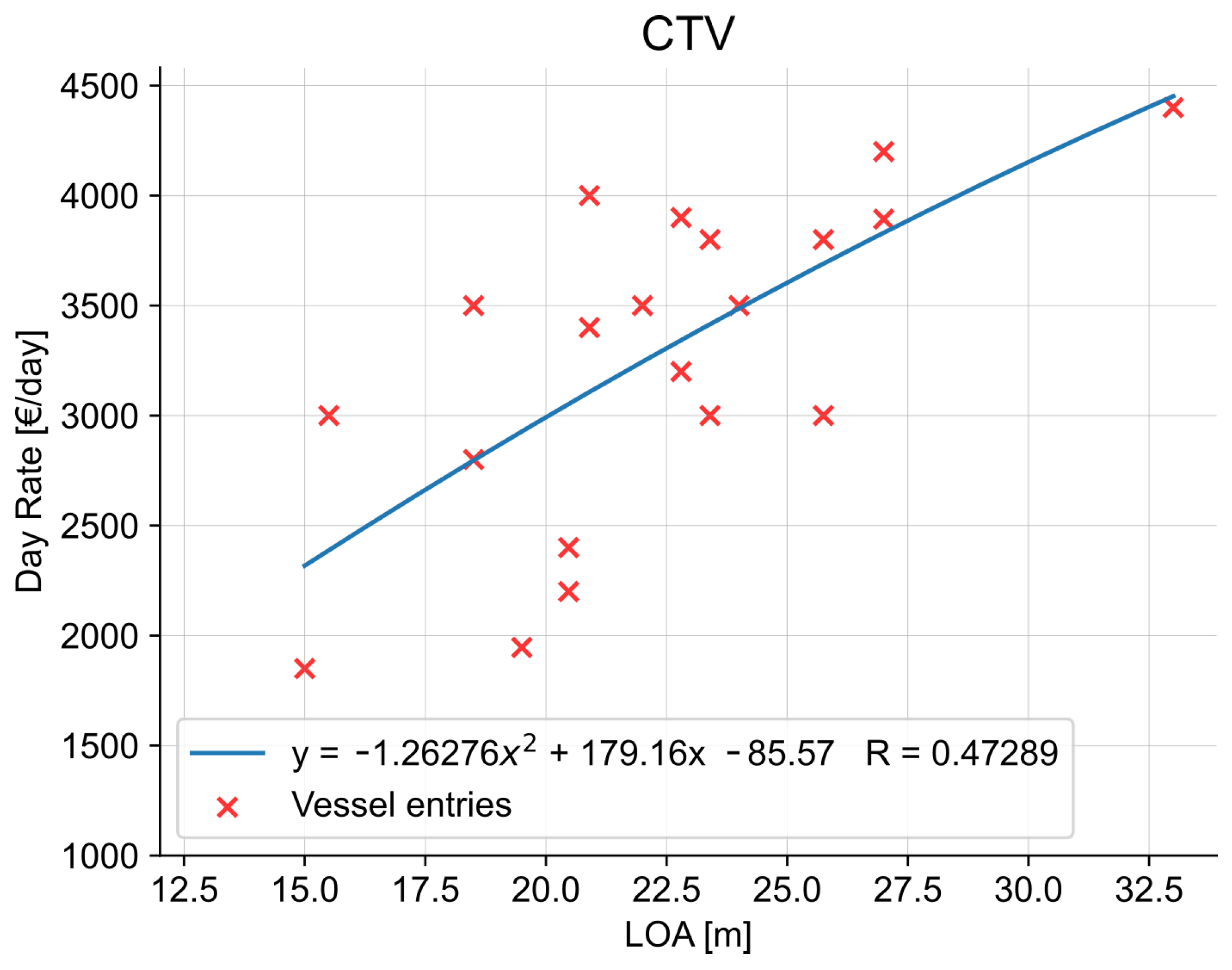
3.6.2. Daily Vessel Charter Rates

The cost of chartering a given vessel depends on several factors, such as vessel characteristics and capabilities, as well as surrounding market conditions. Contract duration and contractual frameworks typically also play a role. Smaller tonnage vessels such as CTVs, tugs, and survey vessels are commonly chartered out on a time charter basis (e.g., BIMCO Supply time [59]) with a clearly defined vessel day rate. However, larger vessels such as jack-up vessels, crane vessels, and cable laying vessels are mostly hired as part of comprehensive service agreements such as EPCI² or T&I³ contracts (e.g., FIDIC or Logic [60]). In order to be able to compare different types of contracts, average daily charter costs that exclude consumables such as fuel and harbour costs, were used.

Vessel characteristics such as age, size, crane capabilities, deck area, dynamic positioning (DP) equipment, and engine power are known to have an impact on the total vessel costs. Based on guidance from Global Renewable Shipbrokers (GRS) [61], a offshore vessel broker, major cost drivers for the vessel charter rates were identified for each vessel type. Even though the vessel charter rates are dependent on a large number of variables, for simplicity and to provide a first cost estimate, vessel charter costs were modeled as a function of a single parameter for each vessel type. As shown in Figure 5, cost functions that model charter day rates for the different vessel types were then derived, based on a curve fitting applied to database points gathered from: (i) DTOcean 1.0 vessel database, (ii) WavEC’s in-house vessel database, (iii) cost figures provided by ECN [62] and GRS, (iv) from industry expert experience. Different regression models, including linear, polynomial, exponential, logarithmic and piece-wise regressions, were adjusted to find a best fit based on the R-squared coefficient, while eliminating fits that result in cost inflections within the analyzed domain. The resulting cost functions were compiled in

Table 11. Daily charter rate regression curves, for different vessel types, in Euros, as a function of their input parameters (x).

Vessel Type	Input Parameter	Domain Validity	Function	R2
Tug	Bollard Pull (tonnes)	$13\le x<25$	$c_{chart}=151.34x-467.47$	0.9611
		$25\le x<70$	$c_{chart}=2.18x+3261.61$
		$70\le x\le 80$	$c_{chart}=508.57x-32186$
Multicat	LOA (m)	$21\le x<28$	$c_{chart}=63.23x+1812.4$	0.96626
		$28\le x<35$	$c_{chart}=916.74x-22086$
		$35\le x\le 42$	$c_{chart}$ = 10,000
AHTS4	Bollard Pull (tonnes)	$70<x\le 338$	$c_{chart}=-8.3\times {10}^{-3}{x}^2+114.90x-261.87$	0.6857
CLV5	Total cable storage (ton)	$565\le x\le$ 10,000	$c_{chart}=2.46\times {10}^{-4}{x}^2+7.25x+$ 53,090	0.4716
CTV6	LOA (m)	$15\le x\le 33$	$c_{chart}=-1.26x^2+179.16x-85.57$	0.4729
DSV7	LOA (m)	$35\le x\le 150$	$c_{chart}$ = 4308.81 exp(0.02x)	0.96580
Guard Vessel	Service speed (knots)	$7\le x\le 24$	$c_{chart}=77.11x+1345.48$	0.99948
Non-propelled Barge	Barge dimensions	$1557\le x\le$ 19,950	$x=ve.LOA*ve.beam*ve.draft$	0.87829
			$c_{chart}=953.92log\left(x\right)-6761.18$
Jack-up vessel	Crane lift capacity (tonnes)	$50\le x<755$	$c_{chart}=64.71x+$ 21,448.41	0.77216
		$755\le x<896$	$c_{chart}=586.18x-$ 372,275
		$896\le x\le 4400$	$c_{chart}=26.83x+$ 128,892
Propelled crane vessel	Crane lift capacity (tonnes)	$4\le x\le 3300$	$c_{chart}=-5.44\times {10}^{-3}{x}^2+88.91x+$ 12,714.58	0.99548
Non-propelled crane vessel	Crane lift capacity (tonnes)	$4\le x<2108$	$c_{chart}=60.62x-9075.34$	0.55486
		$2108\le x<3300$	$c_{chart}=15.74x+$ 85,536.50
PSV8	Free Deck Space (m2)	$30\le x\le 5005$	$c_{chart}=1.005x+8969.85$	1.00
Rock Dumper	Stone cargo capacity (tonnes)	$5400\le x\le$ 69,212	$c_{chart}=3.99x+$ 69,212.41	0.26059
SOV9 with gangway	No. Passengers	$x<60$	$c_{chart}=$ 24,000	N.D.
		$x\ge 60$	$c_{chart}=$ 50,000
SOV gangway relevant	No. Passengers	$x<60$	$c_{chart}=$ 24,000	N.D.
		$x\ge 60$	$c_{chart}=$ 42,000
Survey vessel	LOA (m)	$23\le x\le 56$	$c_{chart}=333.33x-4166.67$	0.66484

. It can be seen that even though charter price variability is not fully explained by a single parameter, important relationships were obtained, with the potential to guide vessel selection decisions.

3.6.3. Daily Vessel Fuel Costs

Given that the considered vessel charter rates excluded fuel costs, vessel fuel consumption had to be estimated. Fuel consumption contributes significantly to the total operation costs, but also to the emissions and carbon footprint of the project. Total vessel fuel consumption depends on several different factors, namely number of engines (main and auxiliary), engine power, engine efficiency, operation duration, mobilized ancillary equipment, transit speed and distance, as well as weather conditions. In order to provide a first fuel consumption estimate, the LMO module calculates the average vessel fuel consumption per day as

$$f_{cs}=\mathrm{TIP}·\mathrm{ALF}·\mathrm{SFOC}·24·\frac{1}{{1000}^2}$$

(3)

In Equation (3), TIP is the vessel’s total installed power (in kW), ALF is the average load factor, and SFOC is specific fuel oil consumption (in g/kWh) [63]. According to the ship broker’s experience in vessel chartering for offshore wind projects, an average load factor of 80%, and a specific fuel oil consumption of 210 g/kWh were indicated as reference values. However, these values may be modified by the user. The daily fuel costs can thus be estimated by multiplying the daily fuel consumption $f_{cs}$ by a reference price of fuel, as shown in Equation (4). In respect to the fuel price $p_{fuel}$, the marine diesel oil (MDO) price in the port of Rotterdam, 515 €/ton, was taken as a reference [64]. However, when running the LMO module, this value may be modified by the user to reflect different fuel prices or even other fuel types such as heavy fuel oil (HFO).

$$c_{fuel}=f_{cs}·p_{fuel}$$

(4)

3.6.4. Equipment Costs

For a given operations, the equipment costs can be simply calculated as the product of the operation duration and the sum of the daily (and/or half-day) renting cost of the selected equipment for that operation. Daily and half-day renting costs figures are available in the equipment databases.

3.6.5. Spare Part Costs

For O&M operations, in case of component failure, the cost of the spare components are calculated using the costs of a new component, as designed by other modules (or introduced by the user) and compiled in the Bill of Materials (BOM).

3.6.6. Port Terminal Costs

Port expenditures are generally port-specific, varying greatly with the type of contract and duration, leased storage area, the size of the vessels, and need for ancillary equipment such as cranes. However, according to the literature, total port expenditures amount on average to about 0.5% of the total costs of offshore wind projects [65]. The port terminal costs were thus included by adding an extra 0.5% to the total operation costs.

3.6.7. Total Operation Costs

For each logistic solution, the total operation costs based on the operation duration $d_{op}$, selected equipment, vessel fleet, port costs, and spare components (for O&M operations), are calculated as described in Equation (5).

$$C_{op}=d_{op}·(c_{ports}+c_{vessels}+c_{equip})+C_{spare}$$

(5)

Based on the total operation costs calculated for each logistic solution candidate, the optimal operation solution that minimizes total costs can be selected for each operation.

3.7. Operation Calendarization

For the installation and decommissioning project life-cycle phases, the operation calendarization functionality is responsible for scheduling the previously identified optimal operations on the project calendar, taking into consideration the project start date, operation net duration, expected weather delays in the considered month, as well as predefined operation sequence. For maintenance operations, the operation calendarization functionality schedules corrective maintenance operations in the aftermath of component failure, and preventive maintenance activities following the predefined preventive maintenance frequency. The periodicity of preventive maintenance operations, as well as the device shutdown requirement, which expresses whether device shutdown is assumed when carrying out the operation, are compiled in the maintenance catalog, as presented in

Table 12. Catalog of preventive maintenance operations, featuring operation name, annual periodicity, and device shutdown requirements.

ID	Name	Periodicity (Years)	Device Shutdown
1	Topside inspection	1	Yes
2	Underwater inspection	2	Yes
3	Mooring inspection	1	Yes
4	Array cable inspection	2	No
5	Export cable inspection	4	No

. The preventive maintenance frequency values may be modified by the user to fit project specific requirements.

In case of component failure, or device shutdown requirement during preventive maintenance, resulting downtime per device is stored. The interrelationships between farm components and the ability of each device to produce and deliver its energy to the grid were represented in a hierarchy structure. This automatically generated tree-like structure, described in detail in [47], allows to evaluate the impacts of a given component failure (e.g., array cable) in the farm energy production (i.e., downtime of respective devices).

4. Case Study

In order to demonstrate the functionalities of the Logistics and Marine Operations module, a case study was developed for the installation of a floating wave energy converter, inspired on Sandia’s Reference Model 3 (RM3) [66]. Sandia’s RM3 device consists of a 260 kW heaving point absorber. The overall design and dimensions are represented in Figure 6.

In the present case study, a deployment location in Europe was selected with similar characteristics (bathymetry and wave energy resource) to the RM3 reference site (Eureka, in Humboldt County, California). The mean reference site wave energy density is 33.5 kW/m. In Figure 7, the selected project site is depicted, as well as relevant nearby ports (stored in the terminal catalog) that were considered during the algorithm’s port selection process. August 1st was specified as the installation starting date due to being the month with best weather conditions.

As a floating device, it was considered that the converter would be transported from port to site by wet towage. Drag-anchors were considered for station keeping. In order to export the generated power to shore, a 3.3 kV export cable with a total length of 6680 m, mostly buried at 0.5 m depth, was considered. The dimensions and characteristics of the subsystems were compiled in

Table 13. Dimensions and characteristics of the floating wave energy converter and sub-systems.

Component	No.	Type	Mass	Length	Width	Height	Draft	Tow draft
Device	1	Floating WEC	680,000 kg	30 m	30 m	42 m	35 m	15 m
Component	No.	Type	Mass	Length	Width	Height
Anchor	3	Drag-anchor	9,535 kg	5.472 m	5.898 m	3.291 m
Component	No.	Material	Mass	Length	Diameter
Mooring line	3	Nylon	4,703 kg	340.7 m	0.146 m
Component	No.	Type	Mass	Length	Diameter	Voltage	MBR	Burial depth
Power cable	1	Export	8,700 kg	6,680 m	0.079 m	3.3 kV	1.15 m	0.5 m

.

Based on the introduced list of components, the LMO module recognized that three operations would be required, in the recommended sequence: (i) installation of the mooring system, (ii) installation of the export cable, and (iii) installation of the device. It is suggested by the algorithm that the mooring system is pre-laid, an increasingly common practice in floating wind projects, followed by the cable installation operation to reduce the risks of cable damage during the mooring installation activities. Finally, the installation of the device consists of wet-towing the converter to site and connecting the pre-laid moorings and umbilical cable.

The results of the LMO module, featuring the selected vessels, durations, and costs for each operation, are shown in

Table 14. Results of the LMO module for the case study.

Operation	Mooring Installation	Cable Installation	Device Installation
Operation sequence	1st	2nd	3rd
Number of vessels	1	1	2
Selected vessels	AHTS	Cable Laying Vessel	Tug, Tug
Selected terminal	Ports Normands Associés-Flamands Sud
Selected equipment	ROV	ROV, plough	ROV
Mobilisation	96.0 h	96.0 h	96.0 h
Total transit	15.6 h	15.2 h	38.1 h
Work at port	67.0 h	24.0 h	2.0 h
Work on site (at sea)	21.0 h	54.0 h	3.0 h
Waiting on weather	163.0 h	85.4 h	0.0 h
Total operation duration	362.6 h	274.7 h	139.1 h
Vessel fuel consumption	548.28 ton	469.13 ton	87.86 ton
Terminal costs	€3345	€5829	€652
Vessel costs	€550,945	€1,035,114	€85,223
Equipment costs	€118,020	€130,614	€45,240
Total operation costs	€672,310	€1,171,557	€131,115

. Leveraging on the port terminal and vessel databases, as the algorithm identified the optimal port-fleet combination in respect on project costs. The Ports Normands Associés, in the north coast of France was selected for all three installation operations. An Anchor Handling Tug Support (AHTS) vessel was recommended for the mooring installation, a Cable Laying Vessel (CLV) for the cable installation (including cable burial), and two tugs for the device installation. Despite being the least energetic month, results suggest that the expected waiting on weather in August is not negligible, representing 41% and 27% of the total expected operation duration for the mooring and cable installation operations, respectively. It can be observed that for a single device, the total installation costs amounts to approximately 1.8 M€. Given that the installation of the cable and moorings are the largest contributors to the total project commissioning costs, significant economies of scale can be expected for projects with a higher number of devices, as multiple components would be installed per trip, avoiding unnecessary transits. The obtained installation cost figures showed good agreement with the RM3 installation cost breakdown, presented in Sandia’s in-depth study [66]. It was found that differences in the results were mainly caused by the mobilization and demobilization assumptions in Sandia’s study, which were not reproduced in LMO. A screenshot of the results page of the LMO module is shown in Figure 8.

5. Conclusions

The present work describes the development of a novel methodology for designing the installation, maintenance, and decommissioning phases of ocean energy projects. Given the sensitivity of given marine operations to weather conditions and its impacts on project costs, a statistical weather window model was developed to estimate potential weather delays. Based on a database of vessels relevant to offshore renewable energy projects, simplified cost functions were produced for each vessel type to estimate the daily charter rates. Employing a systematic approach to infrastructure selection, and leveraging on comprehensive and user-modifiable databases of operations, vessels, port terminals, and equipment, the Logistics and Marine Operations module produces operation plans and optimal infrastructure solutions that satisfy project requirements and minimize total project costs. Tests performed for a case study based on a theoretical floating wave energy converter produced results in good agreement with the detailed study conclusions.

Given its open-source licensing and its community collaborative environment, continuous improvements of the Logistics and Marine Operations module are foreseen. Future research plans include improving functionalities and further demonstrating the developed methodology using data from real ocean energy projects, benchmarking against the outputs of other logistic support tools.

References

1. United Nations Framework Convention on Climate Change. The Paris Agreement. 2015. Available online: https://unfccc.int/sites/default/files/english_paris_agreement.pdf (accessed on 21 January 2020).
2. Gerbaulet, C.; von Hirschhausen, C.; Kemfert, C.; Lorenz, C.; Oei, P.Y. European electricity sector decarbonization under different levels of foresight. Renew. Energy 2019, 141, 973–987. [Google Scholar] [CrossRef]
3. Zeyringer, M.; Fais, B.; Keppo, I.; Price, J. The potential of marine energy technologies in the UK—Evaluation from a systems perspective. Renew. Energy 2018, 115, 1281–1293. [Google Scholar] [CrossRef]
4. Widén, J.; Carpman, N.; Castellucci, V.; Lingfors, D.; Olauson, J.; Remouit, F.; Bergkvist, M.; Grabbe, M.; Waters, R. Variability assessment and forecasting of renewables: A review for solar, wind, wave and tidal resources. Renew. Sustain. Energy Rev. 2015, 44, 356–375. [Google Scholar] [CrossRef]
5. Dias, F.; Renzi, E.; Gallagher, S.; Sarkar, D.; Wei, Y.; Abadie, T.; Cummins, C.; Rafiee, A. Analytical and computational modelling for wave energy systems: The example of oscillating wave surge converters. Acta Mech. Sin. 2017, 33, 647–662. [Google Scholar] [CrossRef] [Green Version]
6. Ocean Energy Forum. Ocean Energy Strategic Roadmap 2016, Building Ocean Energy for Europe. 2016. Available online: https://www.oceanenergy-europe.eu/wp-content/uploads/2017/10/OEF-final-strategic-roadmap.pdf (accessed on 6 November 2020).
7. European Commission. Blue Energy—Action Needed to Deliver on the Potential of Ocean Energy in European Seas and Oceans by 2020 and Beyond. Communication from the Commission to the European Parliament, the Council, the European Economic and Social Committee and the Committee of the Regions. 2014. Available online: https://op.europa.eu/en/publication-detail/-/publication/e4aea330-19b7-42d8-9d5c-0da648e76792 (accessed on 26 July 2021).
8. Shafiee, M. Maintenance logistics organization for offshore wind energy: Current progress and future perspectives. Renew. Energy 2015, 77, 182–193. [Google Scholar] [CrossRef]
9. Thomsen, K.E. Offshore Wind a Comprehensive Guide to Successful Offshore Wind Farm Installation, 2nd ed.; Academic Press: Cambridge, MA, USA, 2014; p. 404. [Google Scholar]
10. Irawan, C.A.; Ouelhadj, D.; Jones, D.; Stålhane, M.; Sperstad, I.B. Optimisation of maintenance routing and scheduling for offshore wind farms. Eur. J. Oper. Res. 2017, 256, 76–89. [Google Scholar] [CrossRef] [Green Version]
11. Carroll, J.; McDonald, A.; Dinwoodie, I.; McMillan, D.; Revie, M.; Lazakis, I. Availability, Operation & Maintenance Costs of Offshore Wind Turbines with Different Drive Train Configurations. Wind Energy 2017, 20, 361–378. [Google Scholar] [CrossRef] [Green Version]
12. Gray, A. Modelling Operations and Maintenance Strategies for Wave Energy Arrays; University of Exeter: Exeter, UK, 2017; p. 315. [Google Scholar]
13. Ahn, D.; Shin, S.C.; Kim, S.Y.; Kharoufi, H.; Kim, H.C. Comparative evaluation of different offshore wind turbine installation vessels for Korean west–south wind farm. Int. J. Nav. Archit. Ocean Eng. 2017, 9, 45–54. [Google Scholar] [CrossRef]
14. Morandeau, M.; Walker, R.T.; Argall, R.; Nicholls-Lee, R.F. Optimisation of marine energy installation operations. Int. J. Mar. Energy 2013, 3–4, 14–26. [Google Scholar] [CrossRef]
15. BVG Associates. Value Breakdown for the Offshore Wind Sector. In Commissioned for Renewables Advisory Board; February 2010; pp. 1–20. Available online: https://assets.publishing.service.gov.uk/government/uploads/system/uploads/attachment_data/file/48171/2806-value-breakdown-offshore-wind-sector.pdf (accessed on 26 July 2021).
16. Poulsen, T.; Hasager, C.; Jensen, C. The Role of Logistics in Practical Levelized Cost of Energy Reduction Implementation and Government Sponsored Cost Reduction Studies: Day and Night in Offshore Wind Operations and Maintenance Logistics. Energies 2017, 10, 464. [Google Scholar] [CrossRef] [Green Version]
17. Low Carbon Innovation Coordination Group. Carbon Innovation Coordination Group Technology Innovation Needs Assessment (TINA) Marine Energy Summary Report; Technical Report; August 2012. Available online: https://assets.publishing.service.gov.uk/government/uploads/system/uploads/attachment_data/file/593459/Technology_Innovation_Needs_Assessment___Marine.pdf (accessed on 26 July 2021).
18. Soukissian, T.; Denaxa, D.; Karathanasi, F.; Prospathopoulos, A.; Sarantakos, K.; Iona, A.; Georgantas, K.; Mavrakos, S. Marine Renewable Energy in the Mediterranean Sea: Status and Perspectives. Energies 2017, 10, 1512. [Google Scholar] [CrossRef] [Green Version]
19. Dalgic, Y.; Lazakis, I.; Turan, O. Vessel charter rate estimation for offshore wind O&M activities. In Proceedings of the 15th International Congress of the International Maritime Association of the Mediterranean IMAM 2013. Developments in Maritime Transportation and Exploitation of Sea Resources, A Coruna, Spain, 14–17 October 2013; pp. 899–907. [Google Scholar] [CrossRef] [Green Version]
20. Walker, R.T.; Van Nieuwkoop-Mccall, J.; Johanning, L.; Parkinson, R.J. Calculating weather windows: Application to transit, installation and the implications on deployment success. Ocean Eng. 2013, 68, 88–101. [Google Scholar] [CrossRef]
21. Gray, A. What Are Operations and Maintenance Simulation Tools?—An Explanation of O&M Models in the Offshore Renewable Energy Sector. August 2020. Available online: https://ore.catapult.org.uk/app/uploads/2020/08/OM_Model_Review_Paper_FINAL.pdf (accessed on 26 July 2021).
22. Welte, T.M.; Sperstad, I.B.; Halvorsen-Weare, E.E.; Netland, Ø.; Nonås, L.M.; Stålhane, M. Operation and Maintenance Modelling. In Offshore Wind Energy Technology; John Wiley & Sons, Ltd.: Hoboken, NJ, USA, 2018; pp. 269–303. [Google Scholar] [CrossRef] [Green Version]
23. James Fisher. Mojo Mermaid. Available online: http://www.mojomermaid.com/ (accessed on 6 November 2020).
24. JBA Consulting. ForeCoast Marine. Available online: https://www.forecoastmarine.com/ (accessed on 6 November 2020).
25. StormGEO Ltd. StormGEO S-Planner. Available online: https://www.stormgeo.com/products/s-suite/s-planner/ (accessed on 6 November 2020).
26. Teillant, B.; Chainho, P.; Raventos, A.; Nava, V.; Jeffrey, H. A Decision Supporting Tool for the Lifecycle Logistics of Ocean Energy Arrays. In Proceedings of the 5th International Conference on Ocean Energy, Halifax, Canada, 4–6 November 2014. [Google Scholar]
27. Teillant, B.; Chainho, P.; Raventos, A.; Sarmento, A.; Jeffrey, H. Characterization of the logistic requirements for the marine renewable energy sector. In Proceedings of the 1st International Conference on Renewable Energies Offshore, Lisbon, Portugal, 24–26 November 2014. [Google Scholar]
28. Rademakers, L.W.M.M.; Braam, H.; Obdam, T.S. Estimating Costs of Operation & Maintenance for Offshore Wind Farms. 2008. Available online: https://repository.tudelft.nl/islandora/object/uuid:ff4a94c7-5f57-4872-aba2-aad622656c16 (accessed on 26 July 2021).
29. Athanasios, K.; Feargal, B. ROMEO-Review of Existing Cost and O&M Models, and Development of a High-Fidelity Cost/revenue Model for Impact Assessment. 2018. Available online: https://www.romeoproject.eu/wp-content/uploads/2018/12/D8.1_ROMEO_Report-reviewing-exsiting-cost-and-OM-support-models.pdf (accessed on 25 January 2021).
30. Hofmann, M.; Sperstad, I.B. NOWIcob—A Tool for Reducing the Maintenance Costs of Offshore Wind Farms. Energy Procedia 2013, 35, 177–186. [Google Scholar] [CrossRef] [Green Version]
31. SINTEF. Decision Support Tools. Available online: https://www.sintef.no/projectweb/marwind/dst/ (accessed on 25 January 2021).
32. Gutierrez-Alcoba, A.; Ortega, G.; Hendrix, E.M.; Halvorsen-Weare, E.E.; Haugland, D. A model for optimal fleet composition of vessels for offshore wind farm maintenance. Procedia Comput. Sci. 2017, 108, 1512–1521. [Google Scholar] [CrossRef]
33. Shoreline. Design Entire Wind Farms by Simulating, Modelling and Analysing Scenarios in a Risk-Free Virtual Environment. Available online: https://www.shoreline.no/solutions/design/ (accessed on 24 January 2021).
34. Dalgic, Y.; Dinwoodie, I.; Lazakis, I.; McMillan, D.; Revie, M. Optimum CTV Fleet Selection for Offshore Wind Farm O&M Activities. In Proceedings of the ESREL 2014, Wroclaw, Poland, 14–18 September 2014; p. 9. [Google Scholar]
35. Dalgic, Y.; Lazakis, I.; Dinwoodie, I.; McMillan, D.; Revie, M.; Majumder, J. The influence of multiple working shifts for offshore wind farm O&M activities—STRATHOW-OM Tool. In Proceedings of the Design and Operation of Offshore Wind Farm Support Vessels, London, UK, 28–29 January 2015; p. 9. Available online: https://www.researchgate.net/publication/271525141_The_influence_of_multiple_working_shifts_for_offshore_wind_farm_OM_activities_-_StrathOW-OM_Tool (accessed on 26 July 2021).
36. Douard, F.; Domecq, C.; Lair, W. A Probabilistic Approach to Introduce Risk Measurement Indicators to an Offshore Wind Project Evaluation—Improvement to an Existing Tool Ecume. Energy Procedia 2012, 24, 255–262. [Google Scholar] [CrossRef] [Green Version]
37. Paterson, J. Metocean Risk Analysis in Offshore Wind Installation. Ph.D. Thesis, University of Edinburgh, Scotland, UK, 2018. Available online: https://era.ed.ac.uk/handle/1842/35981/ (accessed on 15 July 2021).
38. Wave Energy Scotland. Operations and Maintenance Simulation Tool: User Guide. 2017. Available online: https://www.waveenergyscotland.co.uk/media/1182/wes-om-tool-user-guide_rev1.pdf (accessed on 10 December 2020).
39. Sperstad, I.B.; Stålhane, M.; Dinwoodie, I.; Endrerud, O.E.V.; Martin, R.; Warner, E. Testing the robustness of optimal access vessel fleet selection for operation and maintenance of offshore wind farms. Ocean Eng. 2017, 145, 334–343. [Google Scholar] [CrossRef] [Green Version]
40. Grzegorzewska, P. First Results of the Study on the Impact of Open Source|Joinup. Available online: https://joinup.ec.europa.eu/collection/open-source-observatory-osor/news/first-results-study-impact-open-source (accessed on 26 July 2021).
41. Fraunhofer ISI. European Commission: Open Source Study (First Results). Available online: https://openforumeurope.org/wp-content/uploads/2020/11/OFE_Fraunhofer_OS_impact_study_5_Nov.pdf (accessed on 26 July 2021).
42. European Commission. Advanced Design Tools for Ocean Energy Systems Innovation, Development and Deployment|Projects|H2020|CORDIS. 2018. Available online: https://cordis.europa.eu/project/rcn/214811_en.html (accessed on 21 December 2020).
43. The University of Edinburgh. DTOcean FP7-ENERGY EU Project: Optimal Design Tools for Ocean Energy Arrays. Available online: https://cordis.europa.eu/project/id/608597 (accessed on 26 July 2021).
44. The DTOcean Developers. DTOcean: Optimal Design Tools for Ocean Energy Arrays. Available online: https://dtocean.github.io/ (accessed on 11 December 2020).
45. Teillant, B.; Chainho, P.; Vrousos, C.; Charbonier, K.; Ybert, S.; Giebhardt, J. Deliverable 5.6: Report on Logistical Model for Ocean Energy and Considerations. 2016. Available online: https://www.dtoceanplus.eu/content/download/2541/file/DTO_WP5_ECD_D5.6.pdf (accessed on 26 July 2021).
46. Correia da Fonseca, F.X.; Amaral, L.M.B.; Rentschler, M.U.T.; Arede, F.; Chainho, P.; Yang, Y.; Noble, D.R.; Petrov, A.; Nava, V.; Germain, N.; et al. Logistics and Marine Operations Tools—Alpha version. Public Deliverable D5.7, DTOceanPlus, May. Available online: https://www.dtoceanplus.eu/Publications/Deliverables/Deliverable-D5.7-Logistics-and-Marine-Operations-Tools-alpha-version (accessed on 16 July 2021).
47. Yi, Y.; Nambiar, A.; Luxcey, N.; Correia da Fonseca, F.X.; Amaral, L. Reliability, Availability, Maintainability and Survivability Assessment Tool—Alpha Version. Public Deliverable D6.3, DTOceanPlus. 2020. Available online: https://www.dtoceanplus.eu/Publications/Deliverables/Deliverable-D6.3-Reliability-Availability-Maintainability-and-Survivability-Assessment-Tool-alpha-version (accessed on 16 July 2021).
48. Raval, U.R.; Chaita, J. Implementing & Improvisation of K-means Clustering Algorithm. IJCSMC 2016, 5, 191–203. Available online: https://www.ijcsmc.com/docs/papers/May2016/V5I5201647.pdf.
49. Teillant, B.; Raventos, A.; Chainho, P.; Victor, L.; Goormachtigh, J.; Collin, A.; Hardwick, J.; Weller, S.; Guerrini, M.; Giebhardt, J.; et al. Deliverable 5.2: Characterization of Logistic Requirements. 2014. [Google Scholar]
50. Youen, K. Site Characterisation—Alpha Version. Public Deliverable D5.2, DTOceanPlus. 2020. Available online: https://www.dtoceanplus.eu/Publications/Deliverables/Deliverable-D5.2-Site-Characterisation-alpha-version (accessed on 16 July 2021).
51. Chen, Y.; Cao, P.; Mukerji, P. Weather Window Statistical Analysis for Offshore Marine Operations. In Proceedings of the Eighteenth (2008) International Offshore and Polar Engineering Conference, Vancouver, BC, Canada, 6–11 July 2008; The International Society of Offshore and Polar Engineers (ISOPE): Vancouver, BC, Canada, 2008; p. 1. [Google Scholar]
52. Det Norske Veritas (DNV). Modelling and Analysis of Marine Operations. Recommended Practices ed. RP-H103. 2011. Available online: https://rules.dnv.com/docs/pdf/DNVPM/codes/docs/2011-04/RP-H103.pdf (accessed on 26 July 2021).
53. Ochi, M.K. Ocean Waves—The Stochastic Approach; Cambridge University Press: Cambridge, UK, 1998. [Google Scholar] [CrossRef]
54. Goda, Y. Random Seas and Design of Maritime Structures; World Scientific Publishing: Singapore, 2000. [Google Scholar] [CrossRef]
55. Holthuijsen, L.H. Waves in Oceanic and Coastal Waters; Cambridge University Press: Cambridge, UK, 2007. [Google Scholar]
56. Sparks, N.J. IMAGE: A multivariate multi-site stochastic weather generator for European weather and climate. Stoch. Environ. Res. Risk Assess. 2018, 32, 771–784. [Google Scholar] [CrossRef] [Green Version]
57. Yang, X.C.; Zhang, Q.H. Joint probability distribution of winds and waves from wave simulation of 20 years ( 1989–2008 ) in Bohai Bay. Water Sci. Eng. 2018, 6, 296–307. [Google Scholar] [CrossRef]
58. Sasaki, W.; Iwasaki, S.I.; Matsuura, T.; Iizuka, S. Recent increase in summertime extreme wave heights in the western North Pacific. Geophys. Res. Lett. 2005, 32. [Google Scholar] [CrossRef]
59. Kennedys. Notes from the Bar: BIMCO SUPPLYTIME 2017. Available online: https://kennedyslaw.com/thought-leadership/article/notes-from-the-bar-bimco-supplytime-2017/ (accessed on 30 December 2020).
60. Harling, M.; Gard, W.; James, S. Future Trends in Procurement Strategy: The Influence of New Nuclear and Offshore Energy Projects. 2013. Available online: https://uk.practicallaw.thomsonreuters.com/3-549-1845?transitionType=Default&contextData=(sc.Default)&firstPage=true (accessed on 26 July 2021).
61. Global Renewables Shipbrokers. Available online: https://www.grs-offshore.com/ (accessed on 10 January 2021).
62. ECN. Energy Research Centre of the Netherlands. Available online: https://www.ecn.nl/energy-research/index.html (accessed on 4 January 2021).
63. Lundh, M.; Garcia-Gabin, W.; Tervo, K.; Lindkvist, R. Estimation and Optimization of Vessel Fuel Consumption. IFAC PapersOnLine 2016, 49, 394–399. [Google Scholar] [CrossRef]
64. Ship & Bunker. World Bunker Prices. Available online: https://shipandbunker.com/prices (accessed on 16 December 2020).
65. Scottish Enterprise. Oil and Gas ’Seize the Opportunity’ Guides: Offshore Wind. Technical Report SE/4504/May16, Scottish Enterprise. 2016. Available online: https://www.offshorewindscotland.org.uk/media/1116/sesdi-oil-and-gas-div-guide-offshore-wind.pdf (accessed on 26 July 2021).
66. Neary, V.S.; Previsic, M.; Jepsen, R.A.; Lawson, M.J.; Yu, Y.H.; Copping, A.E.; Fontaine, A.A.; Hallett, K.C.; Murray, D.K. Methodology for Design and Economic Analysis of Marine Energy Conversion (MEC) Technologies. 2014. Available online: https://energy.sandia.gov/wp-content/gallery/uploads/SAND2014-9040-RMP-REPORT.pdf (accessed on 21 January 2021).
67. UK Met Office. Cartopy, a Cartographic Python Library with Matplotlib Support for Visualisation. Available online: https://pypi.org/project/Cartopy/ (accessed on 27 April 2021).
Figure 1. Representation of DTOceanPlus tools.
Jmse 09 00810 g001
Figure 2. Working principle of the Logistics module.
Jmse 09 00810 g002
Figure 3. Schematic representation of the inputs to the LMO module.
Jmse 09 00810 g003
Figure 4. Illustrative representation of the non-exceedance probability of waiting on weather for an example operation in a given month.
Jmse 09 00810 g004
Figure 5. Example regression of the daily charter rates for crew transfer vessels (CTVs) as a function of the vessel’s length overall (LOA), based on existing database.
Jmse 09 00810 g005
Figure 6. Sandia’s RM3 floating wave energy reference model design and dimensions.
Jmse 09 00810 g006
Figure 7. Project site in the North sea, including the farm deployment location (in red), relevant ports (blue circles), and optimal port identified by the port selection algorithm (blue star). Map generated in Python using Cartopy library [67].
Jmse 09 00810 g007
Figure 8. Screenshot of the Logistics and Marine Operations module: Installation results. Darker bars in the Gantt chart represent the estimated weather delays for each operation.
Jmse 09 00810 g008